A New Method (MINDED-BA) for Automatic Detection of Burned Areas Using Remote Sensing

Abstract

This work presents a change detection method (MINDED-BA) for determining burned extents from multispectral remote sensing imagery. It consists of a development of a previous model (MINDED), originally created to estimate flood extents, combining a multi-index image-differencing approach and the analysis of magnitudes of the image-differencing statistics. The method was implemented, using Landsat and Sentinel-2 data, to estimate yearly burn extents within a study area located in northwest central Portugal, from 2000–2019. The modelling workflow includes several innovations, such as preprocessing steps to address some of the most important sources of error mentioned in the literature, and an optimal bin number selection procedure, the latter being the basis for the threshold selection for the classification of burn-related changes. The results of the model have been compared to an official yearly-burn-extent database and allow verifying the significant improvements introduced by both the pre-processing procedures and the multi-index approach. The high overall accuracies of the model (ca. 97%) and its levels of automatization (through open-source software) indicate potential for being a reliable method for systematic unsupervised classification of burned areas.

1. Introduction

Fire has played an important role throughout human history, allowing men to transform ecosystems worldwide [1]. Wildfires can be described as biomass burning, with potential impacts on human life, property, and ecosystems [1].

Remote Sensing (RS) methods have been widely applied to incorporate data in fire risk assessment studies. The application of RS methods usually falls into three categories: forecasting systems that predict favorable conditions before fire occurrences; monitoring systems for active fire detection; and monitoring of post-fire conditions, such as burned extent (e.g., burn scar maps) or fire severity [2,3].

Wildfire forecasting systems usually focus on addressing probabilities of ignition and propagation (e.g., [4,5,6]). Such models often combine dynamic variables (e.g., wind, temperature, or moisture) and static variables (e.g., slope, land cover, or proximity to specific features), which may be derived from RS techniques [7,8].

The detection of active fires through RS can be inferred from thermal anomalies, which may be detected from multiple sensors (e.g., MODIS, VIIRS, Landsat series). Rapid burned area estimations may be obtained from short-revisiting-time sensors, although such higher temporal resolutions usually come at the cost of decreased spatial resolutions (e.g., [9,10,11]).

Multispectral indices obtained from optical sensors are amongst the most widely used to obtain variables to evaluate fire hazard (using time series) and to monitor fire-induced changes to vegetation, including burn severity and regeneration [12,13]. Such variables may be used to determine fire risk by using methods that correlate predisposing factors to the occurrence of burned areas, as well as by analyzing how the fire intensity influences ecosystem responses and societal impact [1,14,15,16,17]. Multispectral indices, which may or may not have been developed specifically for the identification of burned areas, often result from a combination of two or more bands, from visible to short-wave infrared ranges [18] (some examples are included in

Table 1. Examples of multispectral indices found in the literature to be used for the detection of burned areas.

Name	Equation		Reference
NDVI	$\mathrm{NDVI}=\frac{\mathrm{NIR}-\mathrm{Red}}{\mathrm{NIR}+\mathrm{Red}}$	(1)	[19]
NDWI	$\mathrm{NDWI}=\frac{\mathrm{Green}-\mathrm{SWIRs}}{\mathrm{Green}+\mathrm{SWIRs}}$	(2)	[21]
NBRs	$\mathrm{NBRs}=\frac{\mathrm{NIR}-\mathrm{SWIRs}}{\mathrm{NIR}+\mathrm{SWIRs}}$	(3)	[22]
NBRl	$\mathrm{NBRl}=\frac{\mathrm{NIR}-\mathrm{SWIRl}}{\mathrm{NIR}+\mathrm{SWIRl}}$	(4)	[22]
NBR2	$\mathrm{NBR}2=\frac{\mathrm{SWIRs}-\mathrm{SWIRl}}{\mathrm{SWIRs}+\mathrm{SWIRl}}$	(5)	[24]
MIRBI	$\mathrm{MIRBI}=10\mathrm{SWIRl}+2-9.8\mathrm{SWIRs}$	(6)	[23]
BAI	$BAI=\frac{1}{{\left(0.1-Red\right)}^2+{\left(0.6-NIR\right)}^2}$	(7)	[29]
BAIMs	$BAIMs=\frac{1}{{\left(0.05-NIR\right)}^2+{\left(0.2-SWIRs\right)}^2}$	(8)	[30]
BAIMl	$BAIMl=\frac{1}{{\left(0.05-NIR\right)}^2+{\left(0.2-SWIRl\right)}^2}$	(9)	[30]

). Such combinations include Visible (VIS) and Near-Infrared (NIR) couples, e.g., the Burned Area Index (BAI) [13], which has been developed specifically for burned area discrimination, or the Normalized Difference Vegetation Index (NDVI) [19,20] and the Normalized Difference Water Index (NDWI) [20,21]. Other combinations consist in grouping Short-Wave Infrared bands (SWIRs) (such as the SWIR1 bands from Landsat sensors) with VIS or NIR bands, e.g., the improved version of BAI (BAIMs) [9] or the Normalized Burn Ratio (NBRs) [22], the latter allowing for discriminating different levels of fire severity. Finally, other indices include longer short-wave infrared bands (SWIRl) (such as the SWIR2 from Landsat sensors), e.g., the alternative versions of BAI (BAIMl) and NBR (NBRl), the Mid-Infrared Burned Index (MIRBI) [23], or the Normalized Burned Ratio 2 (NBR2) combining SWIRs and SWIRl [24].

Multispectral indices can be used for uni-temporal classifications (post-fire) or bi-temporal (pre- to post-fire difference) approaches [12,25]. Among bi-temporal change detections, the Differenced Normalized Burn Ratio (dNBR) is among those with the best performances [26], demonstrating significant correlations with field measurements using images captured within ca. 30 days after fire events [27]. However, as with other indices, it shows poor discrimination between burned areas and other surfaces, such as water, bare soil, or areas with little vegetation [25]. According to [18], the use of indices including SWIRs and SWIRl, has been demonstrated to mitigate errors, particularly commission errors, such as false assignments of clouds, cloud shadows, topographic shadows, and water. Such improvements have been explained by the distinctive spectral signatures of water and burned areas beyond the NIR region, where water tends to absorb longer wavelengths almost completely, while burned forest reflectance remains fairly constant or shows a slightly growing trend (e.g., [28]).

The extraction of thematic information from spectral indices is usually carried out using one or more thresholds, which may be used to define two or more classes (density slicing) [31,32,33]. However, as with any spectral index, finding optimal thresholds is often a difficult task, since they are usually scene-dependent [34,35]. Additionally, the characteristics and spectral reflectance of burned areas may also be highly variable, depending on fire severity or the density of pre-fire vegetation [29,36].

One of the main objectives of this study is to develop and implement a method based on satellite RS imagery and GIS techniques, using an integrated multi-index image-differencing approach aimed at determining burned areas, representing an advancement in respect to the applications of the single indices listed in Table 1. The method develops from the work of [34], and it consists of the analysis of the frequency distribution of a set of index differencing statistics, as well as the combination of different single-index classifications by means of a spatial majority analysis. The method was implemented in a fully automatic procedure and tested for a study area in northwestern Portugal.

2. Methods

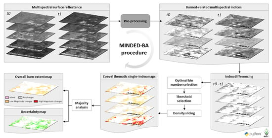
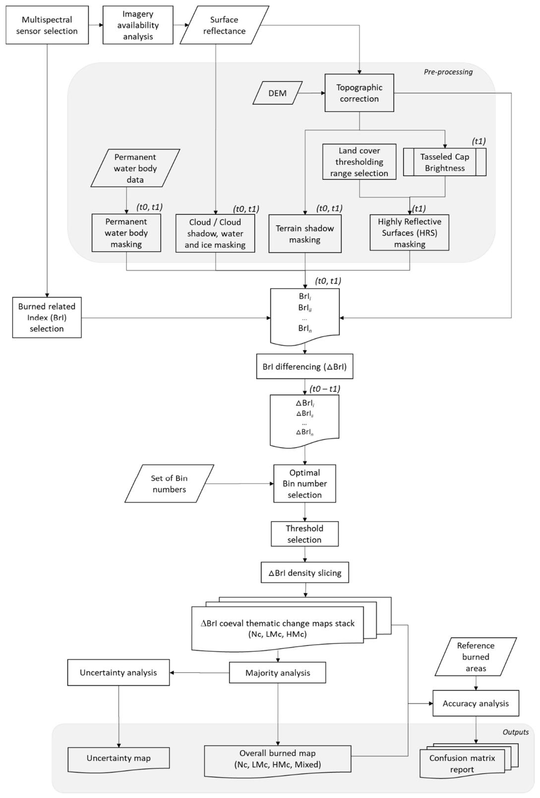
The method developed in this study consists of an adaptation of the Multi-INDEx Differencing (MINDED) method [34], which was originally developed to estimate flood extents. For this work, we have incorporated the same methodological principles, yet with a different purpose: the detection of burned areas. The assembly of the Multi-INDEx Differencing method for Burned Areas (MINDED-BA) follows the workflow illustrated in Figure 1, incorporating Burn-related Indices (BrI). Non-normalized indices introduce data magnitude disparities, which may be exacerbated both in multitemporal analysis contexts and by mathematical derivative operations, potentially requiring additional computational processing and leading to threshold selection issues [34,37]. For these reasons, we decided to implement MINDED-BA by using the following normalized indices: NBRs, NBRl, NBR2, NDVI, and NDWI.

Given the specificities of MINDED-BA, particular considerations should be made for defining the requirements of the satellite images dataset. Firstly, we should perform an analysis to identify the typical fire season period of the study area. In the case of the study area selected to test MINDED-BA (northwestern Portugal), the temperate Mediterranean climate fire season spreads from boreal spring to late boreal summer, particularly during the highest temperature months (i.e., July, August, and September) [38]. This means that the estimation of yearly burned extents may be assumed to be detectable from images acquired prior to (t0) and after (t1) each year fire season. Moreover, in order to minimize false change detections associated with different phenological cycle stages, t0 may be acquired after the end of the previous fire season. This also means that, in a context of a multi-year analysis, every t1 scene may be used as t0 for the following year. The calculation of the BrI should be performed using surface reflectance values, which may be readily available for some sensors (e.g., Landsat series Level 2 or Sentinel-2 Level 2A). Another important issue is to address either t0 or t1 conditions that may result in false detection of burned areas. These might include the occurrence of features such as clouds, cloud shadows, and topographic shadows, as well as water-related changes (e.g., surface water bodies, soil and vegetation water content). Ideally, to minimize such errors, images should include none of these elements. In practice, additional conventional pre-processing steps may be performed in order to minimize the effects of the above conditions (e.g., [39,40,41,42,43,44,45]). Moreover, certain land cover changes (e.g., conversion and/or modifications due to clear-cuts, cropland harvesting, or other soil mobilization practices) may produce index differencing results similar to those from burning. In order to address these cases, specific pre-processing analyses should be performed using remote sensing techniques or other GIS operations based on ancillary information. These analyses represent one of the focuses of the methods developed in this research, and they will be later addressed in Section 4.2.

After the pre-processing phase, the following step of MINDED-BA is to calculate every BrI. This task should be performed (e.g., using the equations of Table 1) for both t0 and t1.

Then, each corresponding ΔBrI may be calculated using Equation (10):

ΔBrI = BrI_t0 − BrI_t1

(10)

Considering each BrI’s specific spectral reflectance bands and the arrangement of Equation (10) (i.e., with t0 as the minuend and t1 as the subtrahend), the following task is to identify the range of values of ΔBrI that are expected to correspond to burn-related changes. For example, considering NDVI, burned areas are usually found to have negative and near-zero values, while green vigorous vegetation is characterized by positive values. Hence, according to Equation (10), those changes from green vegetation to burned result in positive ΔNDVI values. In fact, every other BrI considered in this study performs in a similar way, with recently burned areas corresponding to positive ΔBrI values, whereas longer-term post-fire vegetation regrowth areas are detected as negative values (e.g., [16]).

Then, thematic classifications of changes are obtained by applying thresholding techniques to every ΔBrI. To this end, we considered an procedure analogous to [34], consisting in analyzing each ΔBrI data distribution function (f) and corresponding first and second-order derivative functions, d1f and d2f, respectively. Whenever the shape of f allows separating no-changes from changes (perfectly separated multi-modal values), thresholds may be directly extracted from this distribution curve. This is a conceptual theoretical condition, but in practice, depending on how gradual the transition is between no-change and change conditions, this threshold has to be estimated using either d1f or d2f.

Similarly to [34], we also chose to select two thresholds, T1 and T2, to obtain two classes of magnitude of change, Low-Magnitude change (LMc) and High-Magnitude change (HMc). With these, we expect to detect light burning conditions, such as partially burned canopy, or severe burning conditions, such as complete burning of initially vigorous green vegetation (e.g., forests with high leaf chlorophyll concentration), respectively.

The MINDED-BA workflow continues with the combination of the coeval classifications obtained from the single ΔBrI images. Following the same procedures used with MINDED, we performed a spatial majority analysis, allowing us to obtain the overall burn classifications and to estimate uncertainties.

The final step of the model consists in quantifying accuracies, which may be performed by comparison with either ground truth data or reference ancillary spatial information. In the case of the study area of this paper, we compared the MINDED-BA outputs with the official dataset of yearly burned extents by Portugal’s Institute for Nature Conservation and Forests [46], which was used to provide our reference burned areas (RBA).

All the above steps of MINDED-BA (Figure 1) were also conceptualized with the aim of developing a fully automatic processing tool for rapid and replicable extraction of burned areas from large multitemporal RS imagery datasets. The model was implemented with a GRASSGIS Python script, while the map outputs were obtained with QGIS, both being free and open-source software.

3. Study Area

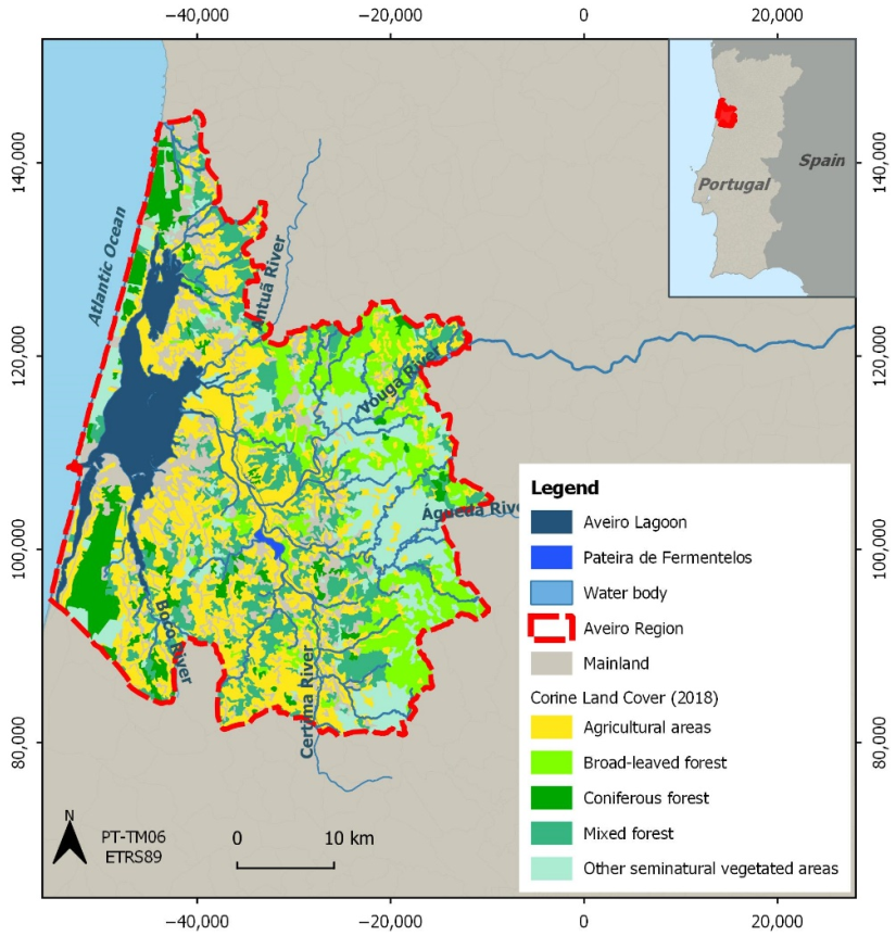
The study area considered in this paper to test the performance of MINDED-BA corresponds to the Aveiro Region, a set of 11 municipalities of the Baixo Vouga subregion (NUTS 3 according to the European Commission Regulation No. 868/2014), located in the northwestern part of continental Portugal (Figure 2). This region is characterized by a temperate Mediterranean climate under maritime influence [38].

The total area covers about 169,286 ha, corresponding to the lower section of the Vouga River Watershed, which is the main freshwater inlet of a wide coastal lagoon, the Aveiro Lagoon. In Figure 2, we can identify other water bodies, including rivers and the Pateira de Fermentelos freshwater lagoon. The choice lof this study area is justified by the recurrence of wildfires and the coexistence of populated territory, along with several important ecological and socioeconomic resources [47]. Additionally, the non-complex topography presents a favorable context for RS methods, such as the application of water-related indices [34]. However, the wide extent and density of water bodies, wetlands and floodplains, represent an additional challenge to test the performance of a wildfire detection method such as MINDED-BA.

According to the Corine Land Cover survey from 2018, forest and semi-natural areas occupy 49% of the study area, consisting of coniferous forest (13%), mostly Pinus pinaster concentrated in flat coastal municipalities; broadleaved forest (26%), mostly of Eucalyptus globulus stands located in the inland and hilly municipalities; and mixed forest (30%). Regarding agricultural areas, they occupy 29% of the study area, among which permanently irrigated land is the most representative land cover class (27%). According to the Regional Forest Plan (National Ordinance n. 58/2019 of February 11), climate change scenarios confirm the tendency for increasing forest fire factors [48].

4. Methodological Application and Results

4.1. Satellite Data Selection

According to the above-described methodological principles of MINDED-BA, the main input of the method consists in multispectral satellite data acquired after the end of each fire season. We used the USGS EarthExplorer portal [49] to search and select multispectral data from the Landsat series (LS) and the Copernicus Open Access Hub [50] for obtaining data from the Sentinel-2A (S2A). Nevertheless, MINDED-BA may be implemented considering any other optical multispectral sensors, for either t0 or t1. In order to analyze the yearly burned extents of our study area from 2000 to 2019, we selected one multispectral image per year from the Landsat series (

Table 2. Multispectral scenes selected for MINDED-BA (LS5—Landsat 5; LS7—Landsat 7; LS8—Landsat 8; S2A—Sentinel-2A).

Fire Season-t1 (Year)	Image Acquisition Date	Satellite	Fire Season-t1 (Year)	Image Acquisition Date	Satellite
-	4 October 1999	LS5	2011	6 November 2011	LS5
2000	22 October 2000	LS5	2012	3 January 2013	LS7
2001	12 December 2001	LS5	2013	10 October 2013	LS8
2002	7 December 2002	LS7	2014	8 December 2014	LS7
2003	10 December 2003	LS7	2015	5 February 2016	LS8
2004	21 January 2005	LS5	2016	6 January 2017	LS8
2005	15 December 2005	LS7	2017	6 November 2017	LS8
2006	27 January 2007	LS5	2018-S	31 December 2018	S2A
2007	22 January 2008	LS7	2018	12 January 2019	LS8
2008	26 September 2008	LS5	2019	30 December 2019	LS8
2009	27 January 2010	LS7	2019-S	10 January 2019	S2A
2010	13 December 2010	LS7

). This list also includes one image from 1999, which has been used as t0 for determining the annually burned extent of the year 2000. As introduced in Section 2, each t1 has been used as t0 for the following reference year, which also facilitated the implementation of the Python script and reduced both computing storage and processing time. Moreover, for sensor comparison purposes, we selected two additional Sentinel-2A (S2A) scenes to be used as alternative references for the fire seasons (t1) of 2018 and 2019. This means that for 2018, MINDED-BA was implemented twice, considering an additional image-differencing couple (2018-S) obtained with a S2A scene (t1), which was subtracted from the original t0 (6 November 2017–LS8). Regarding 2019, MINDED-BA was again implemented twice, but with the additional image-differencing couple (2019-S) determined exclusively with S2A (i.e., for both t0 and t1).

Considering the requirements to calculate each BrI, the multispectral data used as input for MINDED-BA should correspond to surface reflectance values. For this research, we decided to use Landsat Collection 1 Level-2 and Sentinel-2 Level 2A (S2MSI2A) products. For comparison purposes, the S2MSI2A products were downsampled to the same spatial resolution of LS8 (i.e., 30 × 30 m). In addition, to mitigate the adverse effects of non-burn-related changes, our imagery dataset was generally chosen from autumn–winter periods, preferably during low cloud cover and non-flooded conditions.

4.2. Pre-Processing

MINDED-BA is a change detection method tlhat is susceptible to detecting, as side effects, other types of change besides burning. As an index-differencing-based approach, the modal values of the data frequency functions are assumed to represent the condition of no-change, while different types of changes might be inferred depending on which side they are located on in the frequency distribution curve (positive or negative sign). Even though MINDED-BA combines multiple indices, which are obtained from different spectral reflectance bands, other types of change (as those described in Section 2) may have the same sign of burned areas. If not addressed properly, these conditions will result in the occurrence of false positive errors. Pre-processing is therefore advised, which may be implemented from different types of data, including satellite imagery/products, ancillary geographic information, or reference literature values.

For this reason, we performed masking of clouds, cloud shadows, water, and snow features using either the ‘pixel_qa’ band of the Landsat level-2 products [40,51] or the Scene Classification Map (SCL) provided with the S2MSI2A products.

Moreover, considering the susceptibility of permanent water bodies to producing false positive errors and the fact that their spatial position should be relatively stable and well known, we created an additional mask within a buffer of 30 m around water bodies, using official thematic ancillary data [52].

Topographic corrections were performed for every spectral band, using the cosine method [45,53]. Firstly, an illumination model was created for each scene, using the ALOSWorld 3D–30 m (AW3D30) Global DEM provided by the Japan Aerospace Exploitation Agency [54], along with the sun elevation and azimuth acquisition conditions (according to each scene’s metadata). Secondly, we applied the illumination model of each scene, allowing us to mask the shadowed areas and to correct those original reflectance values for pixels directly illuminated from sunlight.

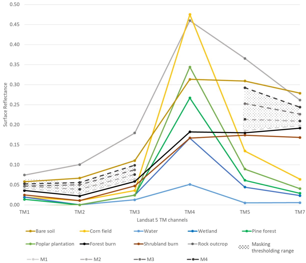
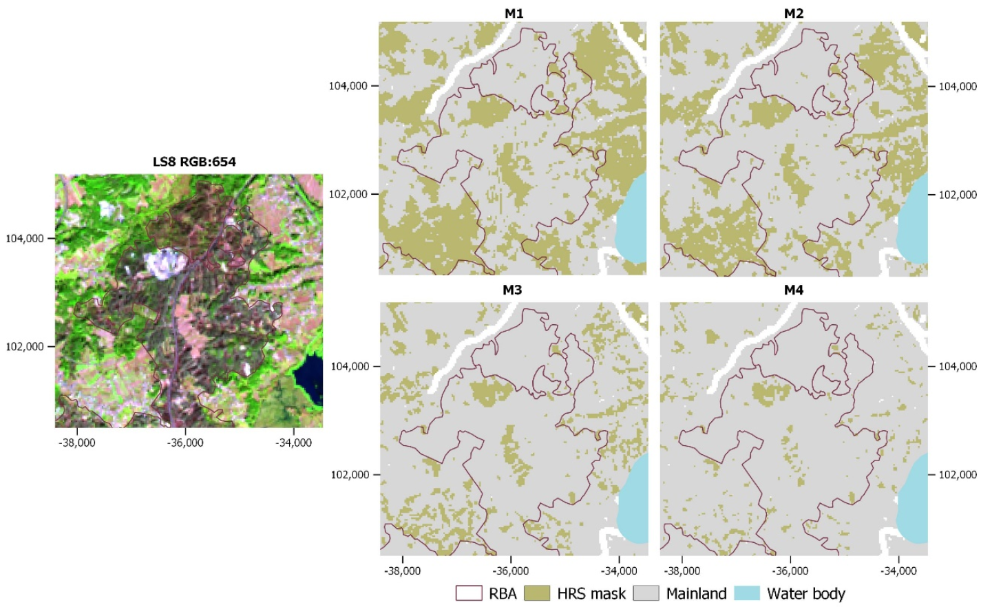
Both burned and bare soil, rock outcrops, and artificial impervious areas are characterized by an absence of chlorophyll, which is otherwise present in green vegetation [25]. When comparing t1 to t0 images, any conversion towards the above-mentioned classes may result in false positive errors. For example, within the study area, corn is one of the most important agricultural crops, which during wintertime (i.e., for most of Table 2 scenes) may show a great variety of spectral signal reflectance, depending on different stages of growth, crop harvesting, or even soil mobilizations prior to new plantings. Some of these conditions result in the conversion of land cover from green vegetation to bare soil, which implies false positive errors. In order to mitigate these error conditions, we analyzed the land cover spectral signatures literature, and we verified that, with the exception of NIR, the reflectance of burned areas, vegetation, wetlands and water is predominantly lower than other highly reflective surfaces (HRS), such as bare soil, rock outcrops and artificial impervious areas [18,21,24,26]. With such considerations in mind, a thresholding range was determined from [28], with the objective of masking HRS in t1. However, since the original reference land cover values are given in top-of-atmosphere (TOA) reflectance, we determined the corresponding ground surface reflectance values, using the 22/10/2000 scene (Table 2). Both the TOA and surface reflectance were obtained from the image DN (Landsat 5 Level 1 and Level 2, respectively), using the band-specific factors provided in the metadata. Then, we sampled clusters of pixels within the range of TOA reflectance values, in order to calculate corresponding average TOA and surface reflectance, allowing us to determine their correlations and obtain the surface reflectance signatures of the different land cover types (Figure 3). Considering the amplitude of the HRS-masking thresholding range, which is maximum for bands TM2, TM3, TM5, and TM7, we integrated this multispectral information calculating the at-satellite Tasseled Cap Brightness (TCB) transformation based on these four bands only (

Table A1. Tasseled Cap Brightness (TCB) at-satellite reflectance coefficients for the red, swir1, and swir2 of Landsat and Sentinel-2 sensors, along with the resulting TCB values for different increments of the thresholding range (M1-M4) for masking highly reflective surfaces (HRS).

Landsat Sensor	Tasseled Cap Brightness (TCB) Coefficients	Masking Thresholds (TCB)
		M1	M2	M3	M4
LS5 (TM)	0.4158 B2 + 0.5524 B3 + 0.3124 B5 + 0.2303 B7 [67]	0.1503	0.1728	0.2002	0.2252
LS7 (TM+)	0.3972 B2 + 0.3904 B3 + 0.2286 B5 + 0.1596 B7 [68]	0.1099	0.1272	0.1479	0.1664
LS8 (OLI)	0.278 B3 + 0.4733 B4 + 0.5080 B6 + 0.1872 B7 [69]	0.1692	0.1942	0.2261	0.2564
S2A (MSI)	0.3813 B3 + 0.3437 B4 + 0.2396 B11 + 0.1949 B12 [70]	0.1155	0.1327	0.1538	0.1728

). Different TCB values were calculated for a series of four increments of the thresholding range (M1-M4; Figure 3). Even though the diagram of Figure 3 refers to Landsat 5, we considered the same spectral signatures regardless of the sensor, as these latter bands have a good spectral correspondence (e.g., [55,56,57]). The four TCB increments were used to mask the t1 dataset. In principle, we expected M2 and M3 to maximize the separation between burned areas and HRS. However, as verified in Figure 4, in comparison to the false color composite of Landsat 8 bands 654 (in RGB), we found M1 to produce slight improvements in masking HRS, without compromising the detection of burned areas, thus justifying its use in the further steps of MINDED-BA.

4.3. Index Calculation and Differencing

After pre-processing every multispectral band, we calculated all BrI for each scene, i.e., for both t0 and t1, using the equations of Table 1. As expected, the scale of results obtained ranges from −1 up to 1, as normalized indices (i.e., NBRs, NBRl, NBR2, NDVI, and NDWI) were used.

Then, considering Equation (10), we calculated each ΔBrI, using the BrI values for t0 and t1. As previously mentioned, for sensor comparison purposes, the implementation of MINDED-BA was performed twice for 2018 and 2019, using both LS8 and S2A data. The scale of every ΔBrI ranges between −2 and 2.

4.3.1. Selection of Optimal Number of Bins and Threshold

For the threshold selection procedure of MINDED-BA, we calculated both first-order derivatives (d1f) and second-order derivatives (d2f) from the ΔBrI frequency distributions. The computational processing was performed considering the effect of data binning. In fact, we verified that by considering different binning intervals, we were experiencing significantly different results. Within a range of higher bins, we observed higher frequency oscillations, while using smaller bins would substantially reduce this effect, until reaching a point where d1f and d2f start losing local extrema, consequently preventing any threshold selection. We also found that by using smoothing techniques based on mobile averaging (according to [34]), we could reduce local noise, while also reducing the overall signal of the functions. Additionally, smoothing seemed to affect the shape of d1f and d2f, resulting in shifting of modal values in the horizontal axis, eventually causing the signal to become flat, which would have a negative effect in the threshold selection procedure. For these reasons, we developed a new approach to better determine which number of bins would provide the best signal-to-noise combination, for both d1f and d2f.

We started by defining a representative set of numbers of bins to be analyzed. Equation (11) allows extracting any amount (j) of numbers of bins (n) equally spaced in a base 10 logarithmic scale by a constant factor (a):

$$Bi{n}_n=\{\begin{array}{c}{10}^n, n=1\\ {10}^{1+a\left(n-1\right)}, n\ne 1\end{array},1\le n\le j, \left(j,n\right)\in \mathbb{N}, \left(a>0\right)\in ℝ$$

(11)

Using Equation (11), we extracted a sample of 15 numbers of bins (i.e., j = 15 and n from 1 to 15), equally spaced by a constant a = 0.15, resulting in the following set: 10, 14, 20, 28, 40, 56, 79, 112, 158, 224, 316, 447, 631, 891, and 1259.

Afterwards, the optimal bin number selection was implemented for each ΔBrI d1f and d2f. This procedure was empirically performed considering Equation (12), which is based on the assumption that statistical noise is associated with erratic oscillations of these functions:

$$Bin\_ratio=\frac{total\_cs}{{\#}_{\left(>mv\right)}}$$

(12)

where ${\#}_{\left(>mv\right)}$ is the number of values of the variable greater than the modal value of the ΔBrI frequency distribution, and total_cs is the total number of consecutive ΔBrI values with the same slope sign, including both consecutive positive and negative slopes. We calculated the Bin_ratio of Equation (12) for each number of bins of every ΔBrI d1f and d2f. The highest Bin_ratio is assumed to correspond to the number of bins providing the optimal signal-to-noise combination.

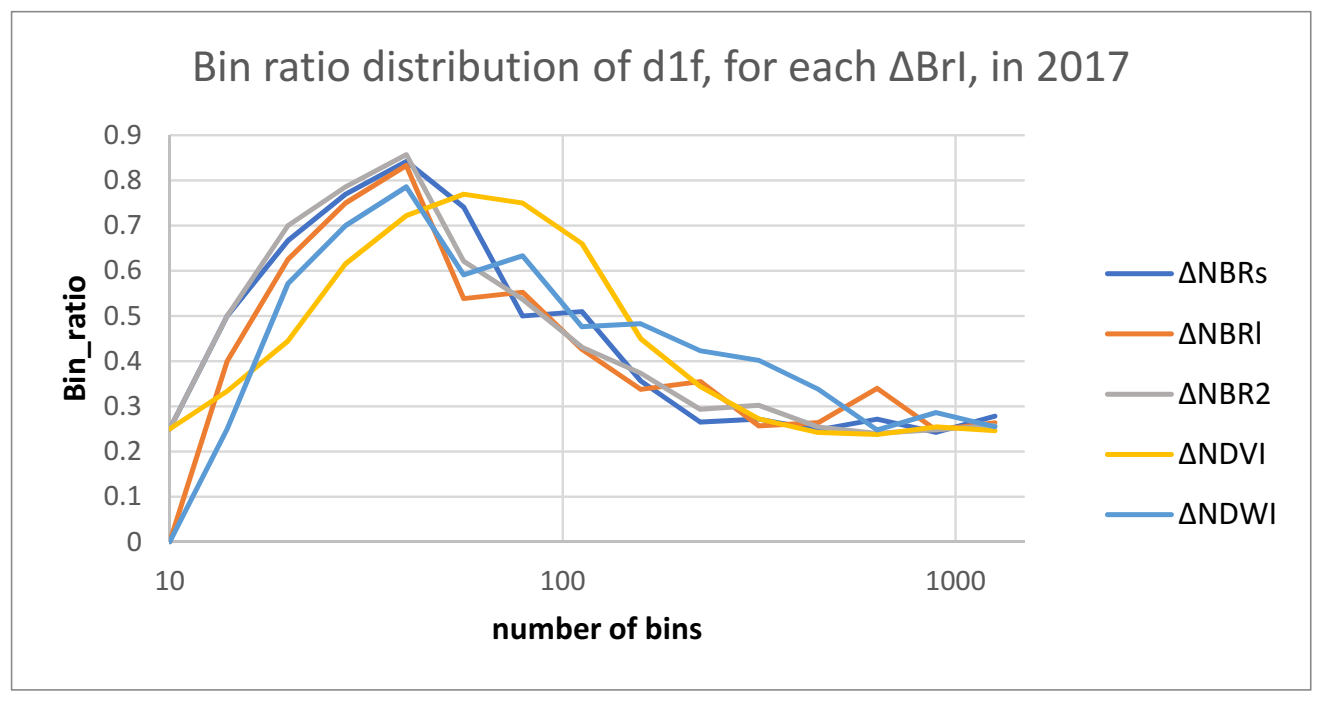
Figure 5 illustrates an example of the Bin_ratio distribution of the d1f of every ΔBrI corresponding to the image difference of 2017. In this case, we verify that for every ΔBrI, an optimal number of bins may be selected corresponding to the modal value of the Bin_ratio distribution. We also found that the distribution functions achieve minimum stable values after ca. 447, further demonstrating the representability of both the selected sample size and numbers of bins.

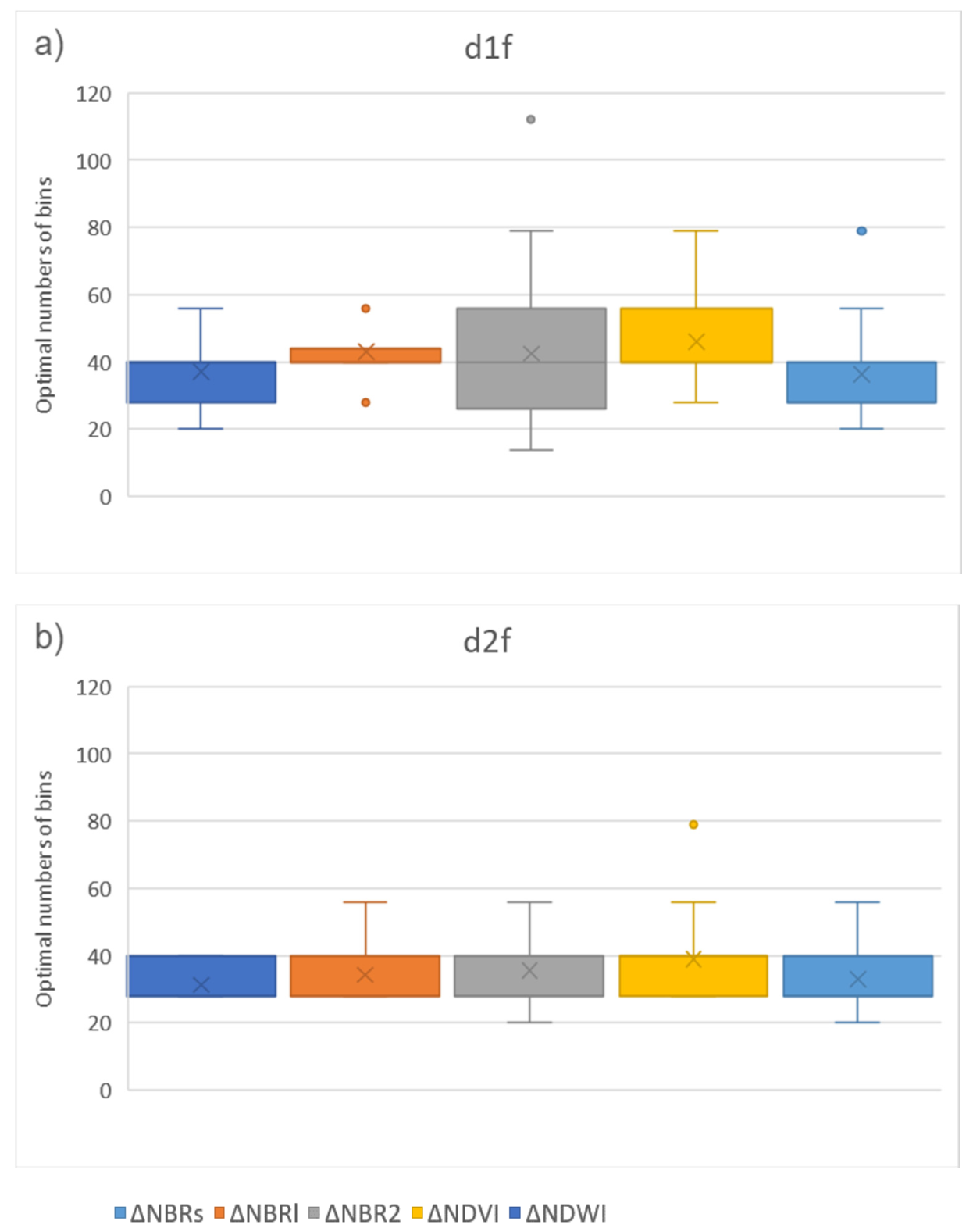
The entire set of values for the optimal number of bins per year, ΔBrI, and derivative order (d1f and d2f) is shown in

Table A2. Optimal numbers of bins, for each ΔBrI d1f and d2f.

	df1					df2
	ΔNBRs	ΔNBRl	ΔNBR2	ΔNDVI	ΔNDWI	ΔNBRs	ΔNBRl	ΔNBR2	ΔNDVI	ΔNDWI
2000	40	40	40	40	20	28	28	28	40	56
2001	40	40	14	40	56	40	28	20	28	40
2002	40	56	20	28	28	28	40	28	40	28
2003	40	40	28	40	40	28	40	28	28	28
2004	28	40	28	56	40	28	40	28	28	28
2005	40	56	28	56	28	28	28	28	40	28
2006	28	28	40	28	40	28	56	40	28	28
2007	28	40	56	40	28	28	40	40	28	28
2008	40	40	40	40	28	40	28	28	40	28
2009	40	40	20	40	28	40	28	28	40	56
2010	20	40	20	56	28	28	28	28	28	28
2011	40	56	56	40	28	28	28	56	40	28
2012	28	56	28	40	28	40	28	20	40	40
2013	40	40	79	56	79	40	28	56	40	20
2014	40	40	112	40	28	40	56	56	28	40
2015	40	40	79	56	28	28	28	56	28	28
2016	56	56	28	56	40	28	40	28	79	28
2017	40	40	40	56	40	28	40	40	40	40
2018	40	40	40	79	40	28	40	40	56	28
2018-S	28	40	79	40	40	28	28	40	40	28
2019	40	40	40	28	28	28	28	40	56	40
2019-S	40	40	20	56	56	28	28	28	40	28

. In Figure 6, the same data are represented as box-plot diagrams. We found the optimal number of bins to vary depending on the ΔBrI, derivative order, and scene. In general, the d1f of ΔNBRs appears to be less variable and, together with the ΔNDWI, is handled better with lower numbers of bins. For ΔNBR2 and ΔNDVI, the optimal numbers of bins of d2f are generally lower than those of d1f, with ΔNBR2 showing the highest variability for d1f. Despite having analyzed a wide range of numbers of bins (10-1259), we highlight that inter-quartile range of the entire set of optimal numbers of bins is concentrated into a very small range (28–56). This suggests the occurrence of a common tendency to stability of the optimal numbers of bins independently of the ΔBrI considered.

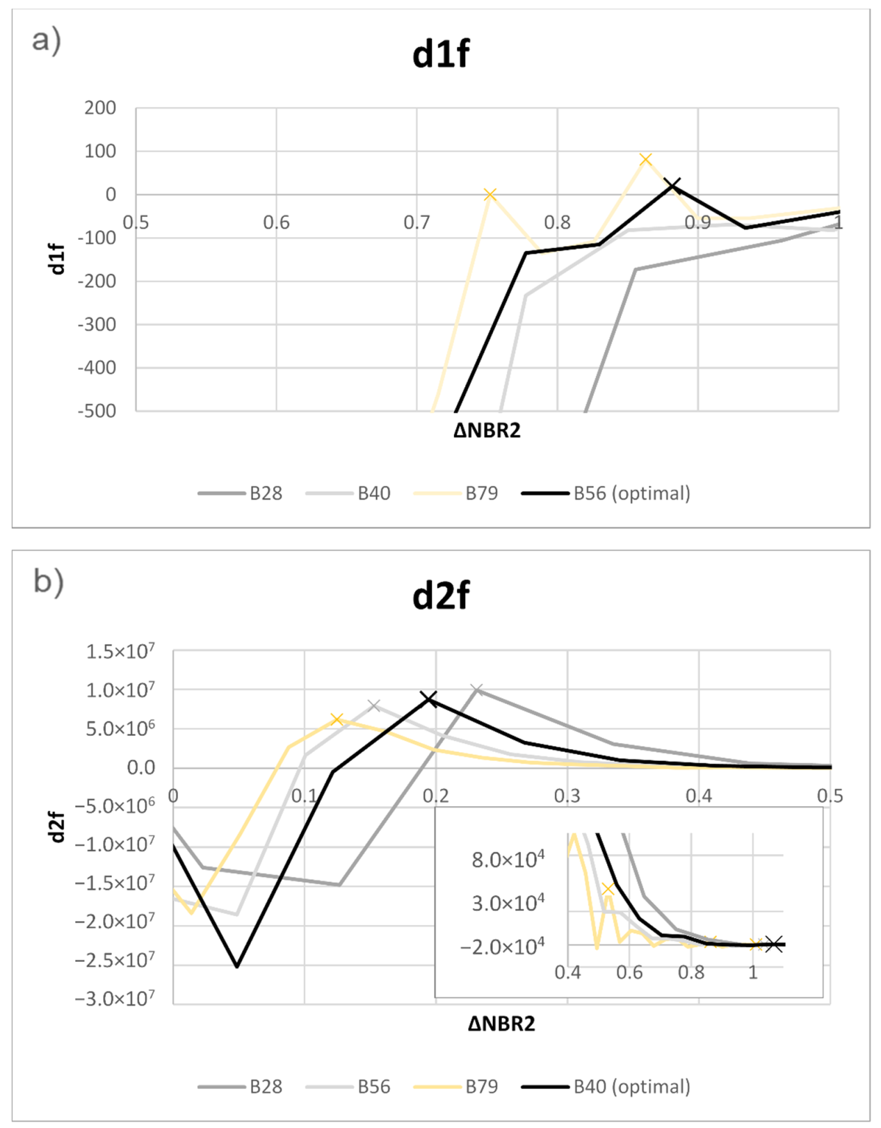
Figure 7 illustrates the d1f and d2f functions obtained from different numbers of bins. This example corresponds to the ΔNBR2 of 2007, in which we can observe the optimal numbers of bins (i.e., 56 for d1f and 40 for d2f), alongside other consecutive non-optimal values. Considering the example of Figure 7a, where thresholds may be identified as changes to positive d1f values, the representation for 79 bins seems to have the highest apparent signal, as the result of a lower compression of the ΔNBR2 frequency statistics. However, it also shows the highest oscillations, compared to other representations, implying the detection of additional thresholds with lower ΔNBR2 values. The latter would potentially lead to increase false positive detection (overestimation of changes). Also, in Figure 7a, due to the downsampling effect of numbers of bins 28 and 40, no thresholds could be extracted from d1f, which would potentially increase false negative errors (underestimation of changes). Regarding Figure 7b, where thresholds correspond to local maximums after a change to positive d2f, we also verify that higher numbers of bins imply lower threshold values. However, higher numbers of bins also increase local noise, increasing the number of local maximums and consequent thresholds (e.g., number of bins 79 from ΔNBR2 0.4 to 0.9). In both cases, the optimal numbers of bins seem to provide the best apparent compromise between signal and noise.

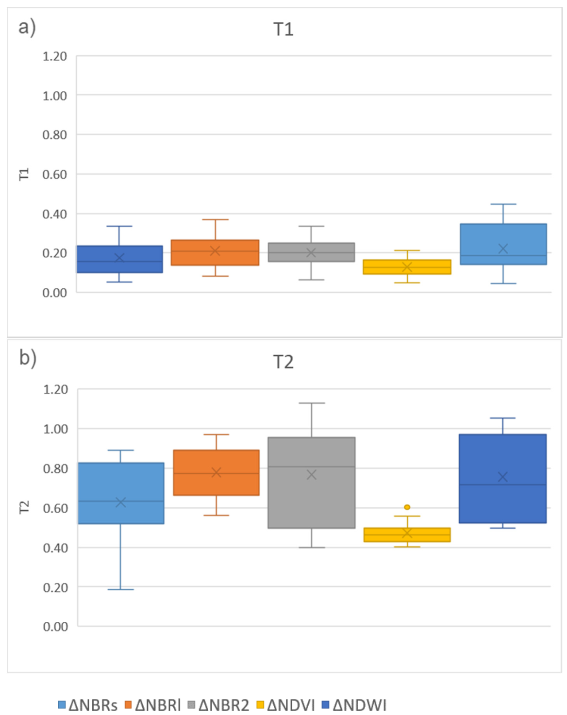
The thresholds extracted from each optimal number of bins are listed in

Table A3. Thresholds T1 and T2 (if any), obtained from each ΔBrI.

	ΔNBRs		ΔNBRl		ΔNBR2		ΔNDVI		ΔNDWI
	T1	T2	T1	T2	T1	T2	T1	T2	T1	T2
2000	0.09	0.56	0.14	-	0.20	-	0.11	-	0.06	0.50
2001	0.10	0.63	0.21	0.97	0.34	-	0.14	-	0.22	-
2002	0.16	-	0.24	0.90	0.27	-	0.09	0.45	0.23	-
2003	0.14	-	0.16	0.77	0.25	1.13	0.16	-	0.17	-
2004	0.30	-	0.33	0.94	0.31	-	0.20	-	0.43	-
2005	0.22	0.85	0.31	0.60	0.25	-	0.14	0.43	0.19	-
2006	0.22	0.89	0.20	0.66	0.19	0.96	0.17	-	0.34	-
2007	0.10	0.63	0.16	0.86	0.19	0.88	0.21	-	0.04	-
2008	0.24	0.48	0.33	-	0.24	-	0.10	0.42	0.45	-
2009	0.10	0.35	0.12	-	0.19	0.88	0.12	0.43	0.08	0.52
2010	0.12	-	0.21	-	0.22	1.07	0.21	-	0.15	-
2011	0.21	-	0.24	-	0.23	-	0.09	0.48	0.36	-
2012	0.11	0.56	0.18	0.66	0.26	-	0.06	-	0.18	0.71
2013	0.27	0.84	0.37	-	0.22	0.46	0.12	0.40	0.37	0.97
2014	0.05	0.60	0.08	0.56	0.12	0.40	0.15	-	0.09	-
2015	0.28	-	0.29	-	0.20	0.73	0.17	-	0.36	1.05
2016	0.06	0.19	0.10	0.75	0.09	0.72	0.05	0.50	0.20	-
2017	0.33	0.77	0.21	0.74	0.16	0.92	0.16	0.47	0.15	-
2018	0.13	-	0.13	0.82	0.07	0.48	0.07	0.48	0.19	0.88
2018-S	0.23	-	0.24	-	0.15	-	0.07	0.45	0.34	-
2019	0.15	-	0.14	0.87	0.11	0.56	0.11	0.56	0.12	-
2019-S	0.23	0.81	0.26	-	0.17	-	0.15	0.60	0.17	0.65

and represented in Figure 8 as box-plot diagrams. For the threshold selection, we chose the lowest threshold values for T1 and T2, independently of d1f and d2f. In some cases, only one threshold could be extracted, while in others, more than two thresholds could be found. This means that, in the example of Figure 7, T1 was obtained by d2f (0.19), while T2 was obtained by d1f (0.88). Table A3 and Figure 8 show that T1 values are less variable in comparison to T2. The ΔNDVI T2 values are also significantly lower than the remaining ΔBrI. The ΔNDWI value was among the most variable, for both T1 and T2.

4.3.2. Single ΔBrI Results

After extracting one or two thresholds for each ΔBrI, we performed density slicing to estimate different burn-related change magnitudes, which are summarized in

Table 3. Summary of single ΔBrI results, given as area (in hectares) for each class (Nc—no change; LMc—low-magnitude change; HMc—high-magnitude change).

	ΔNBRs			ΔNBRl			ΔNBR2			ΔNDVI			ΔNDWI
Year	Nc	LMc	HMc	Nc	LMc	HMc	Nc	LMc	HMc	Nc	LMc	HMc	Nc	LMc	HMc
2000	96,808	7463	33	99,907	4509	-	103,706	577	-	97,821	6483	-	102,063	2357	2
2001	86,634	10534	19	91,396	4624	1	94,736	1279	-	90,757	6492	-	96,001	1186	-
2002	111,021	5431	-	111,939	2263	3	111,647	2555	-	112,082	4395	44	112,189	4262	-
2003	112,256	5838	-	110,062	5061	2	112,376	2751	3	113,760	4373	-	113,439	4655	-
2004	96,583	6735	-	95,041	5831	5	97,697	3184	-	98,810	4554	-	98,604	4694	-
2005	84,091	7736	26	85,004	3411	2142	85,706	4848	-	82,453	7832	1 768	91,206	629	-
2006	91,977	6718	10	88,952	8326	464	92,817	4923	1	95,200	3514	-	93,914	4790	-
2007	86,524	6971	14	88,631	4547	0	90,837	2339	1	89,682	3832	-	92,397	1111	-
2008	81,004	3726	308	83,051	1931	-	83,446	1537	-	82,734	2301	4	81,591	3447	-
2009	87,619	7898	871	87,989	7986	-	94,680	1291	3	88,142	8019	256	94,586	1801	1
2010	85,104	6177	-	87,502	2748	-	87,723	2522	3	87,596	3696	-	89,881	1400	-
2011	86,086	9829	-	86,266	8867	-	90,874	4256	-	86,598	9310	137	89,617	6298	-
2012	98,776	8283	570	101,703	4176	497	104,778	1592	-	98,752	8919	-	105,730	1897	2
2013	77,805	8076	134	80,015	4774	-	77,684	6777	321	78,779	6208	319	80,392	5442	170
2014	93,499	8934	7	95,621	5672	27	98,429	2512	367	97,234	5281	-	101,763	672	-
2015	96,771	4487	-	95,594	4553	-	93,186	6949	0	98,529	2792	-	96,918	4300	24
2016	89,787	10,910	10 277	94,283	16,451	239	102,827	8145	1	88,387	22322	68	110,191	739	-
2017	85,835	6853	298	77,007	14,692	1 287	78,300	14677	9	81,918	9378	131	89,001	3945	-
2018	98,014	6355	-	99,239	5123	8	99,576	4794	-	96,335	7957	60	103,823	505	2
2018-S	103,529	4810	-	104,965	3374	-	103001	5338	-	102602	5656	86	106,748	1579	-
2019	106,920	5099	-	106,468	5533	18	109,556	2463	-	105,135	6793	979	111,247	739	-
2019-S	111,793	4999	36	112,485	4342	-	115691	1136	-	109,466	7323	764	115,820	1004	4

. Following the approach of [34], every pixel lower than T1 was classified as No change (Nc). Those in between T1 and T2 were classified as Low-Magnitude change (LMc), while pixels above T2 were classified as High-Magnitude change (HMc). From Table 3, we can verify the consistency of Nc areas as the clear majority, followed by LMc areas, and finally HMc areas, the latter being always dependent on the detection of a T2. Regarding the years of 2018 and 2019, which were determined twice using different satellite sensors, we found similar results, with LS8 overestimating change areas in comparison to S2A (particularly for ΔNBRs and ΔNBRl).

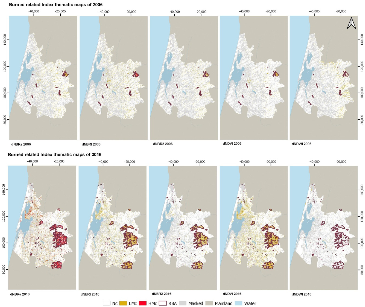
The yearly burn-related maps from each ΔBrI are exemplified in Figure 9, showing results for 2006 and 2016, where the single-index classifications are compared to the RBA [46].

From Table 3, we can verify that ΔNDWI tends to detect the least change, both in terms of LMc and HMc areas. Moreover, and as verified in the examples of Figure 9, such changes tend to be clearly outside the limits of the RBA. Considering these discrepancies and the overall purpose of MINDED-BA, we decided to exclude ΔNDWI from further steps of the model. As for the remaining ΔBrI, we verify that ΔNBRs seem to be the most sensitive to detecting both magnitudes of change, particularly in comparison to ΔNBR2. In Figure 9, most HMc areas were detected by ΔNBRs and ΔNBRl, with the clear majority occurring within the limits of the RBA. However, these same indices also seem to be more affected by image noise (i.e., apparently random distributed pixels), particularly for LMc areas. In 2006, several LMc pixels are detected along the lower Vouga River by ΔNBRs, ΔNBRl, and ΔNDVI. As for 2016, we also verify the occurrence of several change pixels outside the RBA (mostly LMc areas), which, based on visual inspection of imagery and ancillary data [58], are particularly incident in corn plantations, on the banks of the northern branch of the Aveiro Lagoon.

4.3.3. MINDED-BA Maps

After performing density slicing for each ΔBrI, we combined the yearly classifications of ΔNBRs, ΔNBRl, ΔNBR2, and ΔNDVI through a majority analysis. This means that the overall MINDED-BA map classes Nc, LMc, or HMc were given whenever there was a majority among the coeval ΔBrI maps. For every non-majority combination, pixels were classified as ‘Mixed’. Nevertheless, two particular conditions have been addressed. The first one corresponds to the case of 2LMc+2HMc coeval classifications, which were considered to likely describe a burn-related change, and therefore they were classified as LMc areas. The second condition corresponds to 2Nc+LMc+HMc. Despite the relative majority of Nc class, these were classified as Mixed, as the overall combination consists of a tie between no-change and change.

The overall results from the majority analysis procedure are shown in

Table 4. Overall MINDED-BA results, from 2000 to 2019.

Year	Nc		LMc		HMc		Mixed
	Area (ha)	%	Area (ha)	%	Area (ha)	%	Area (ha)	%
2000	98,621	94.6	3645	3.5	-	0.0	2017	1.9
2001	90,116	93.9	2774	2.9	-	0.0	3097	3.2
2002	111,044	97.3	1573	1.4	0	0.0	1551	1.4
2003	110,206	95.8	2232	1.9	-	0.0	2651	2.3
2004	95,484	94.7	2572	2.6	-	0.0	2791	2.8
2005	83,683	92.4	4678	5.2	403	0.4	1777	2.0
2006	90,709	92.8	3186	3.3	3	0.0	3832	3.9
2007	88,350	94.8	2235	2.4	0	0.0	2590	2.8
2008	82,556	97.1	1349	1.6	1	0.0	1077	1.3
2009	87,895	91.6	5074	5.3	49	0.1	2956	3.1
2010	86,722	96.1	1787	2.0	-	0.0	1736	1.9
2011	86,074	90.5	5741	6.0	-	0.0	3312	3.5
2012	99,896	93.9	3618	3.4	191	0.2	2630	2.5
2013	78,493	92.6	4329	5.1	52	0.1	1863	2.2
2014	94,917	93.7	3253	3.2	1	0.0	3084	3.0
2015	95,741	95.7	2397	2.4	-	0.0	1934	1.9
2016	91,456	82.4	15,974	14.4	112	0.1	3390	3.1
2017	79,573	85.6	8897	9.6	287	0.3	4197	4.5
2018	98,364	94.3	4089	3.9	0	0.0	1885	1.8
2018-S	104,233	96.2	2153	2.0	-	0.0	1945	1.8
2019	106,522	95.1	4119	3.7	-	0.0	1345	1.2
2019-S	112,114	96.0	3749	3.2	0	0.0	964	0.8

. In general, we observe Nc to be the most representative class (mostly above 90%), while HMc areas are the clear minority. LMc areas tend to be the second largest, which are sporadically exceeded by the Mixed class. From this entire set, 2016 was the year with the largest changes, particularly in LMc areas, followed by 2017 and 2011. In contrast with the above results, we observe that Mixed class areas remain relatively constant throughout the entire dataset, never exceeding 5% of the overall area.

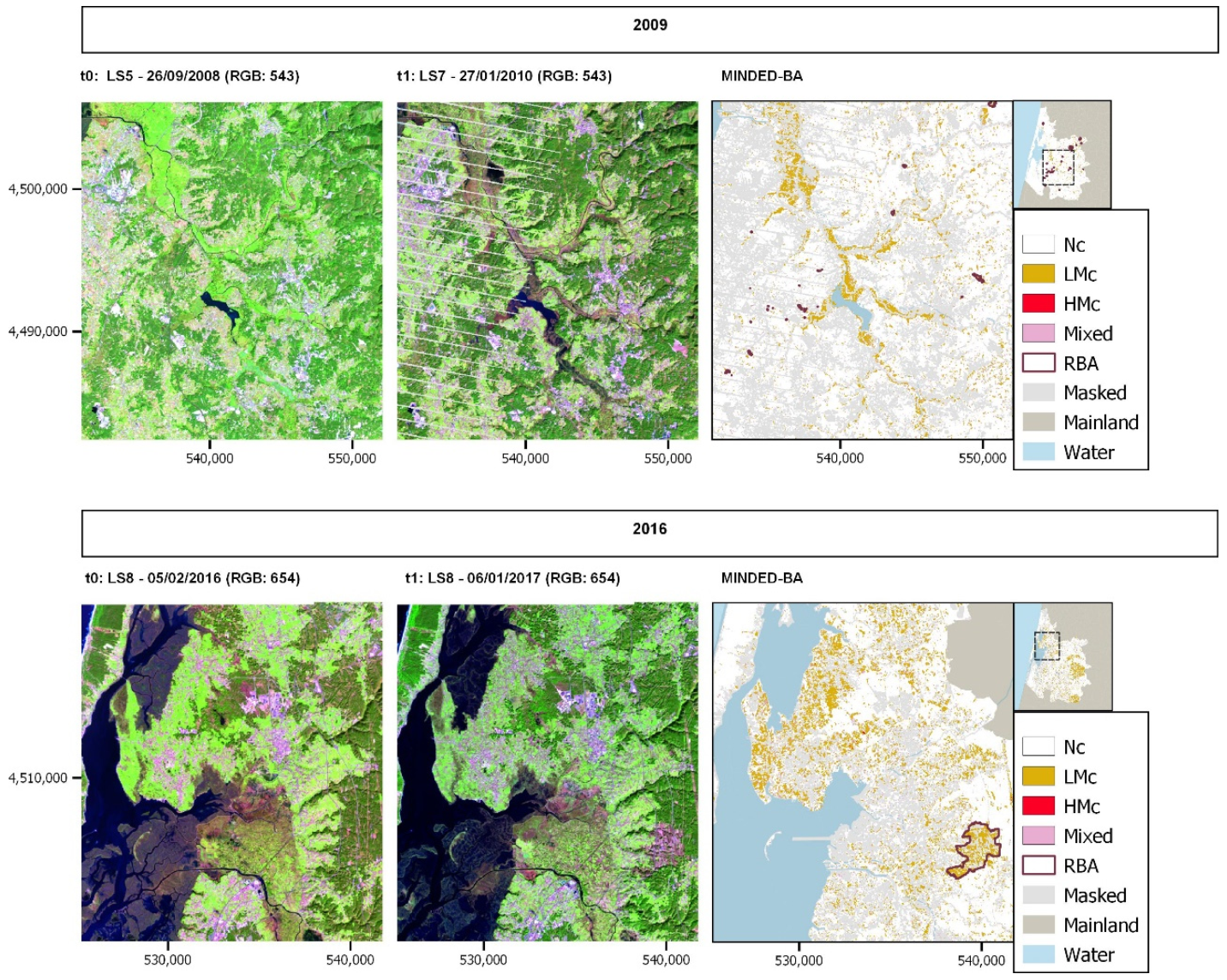
Figure 10 shows the MINDED-BA maps obtained with the Landsat series, from 2000 to 2019. The thematic classifications obtained from the model are displayed along with the RBA, indicating a good correspondence between both datasets. These maps allow us to observe that Mixed pixels tend to be located within burned areas.

Nevertheless, we also verify the occurrence of several LMc areas outside the RBA extents. In Figure 11, the false color composites allow us to identify flooded or highly water-saturated areas in brown, bare soil areas as light pink, whereas burned areas, as obtained by the RBA, correspond to tones similar to the above classes. The MINDED-BA maps detect LMc areas either around water bodies (e.g., 2000, 2009, 2014, and 2019), or in presumably non-burned agriculture fields (e.g., 2016) such as corn plantations. These changes may be interpreted as a consequence of soil water content variations, different stages of plant growth, as well as crop harvesting effects, which cause false positive errors resulting from similar ΔBrI to burned areas.

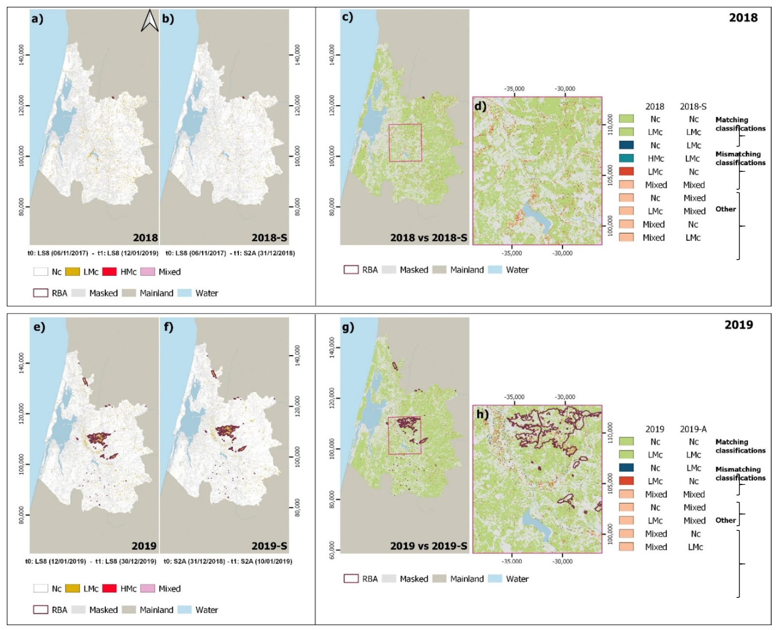
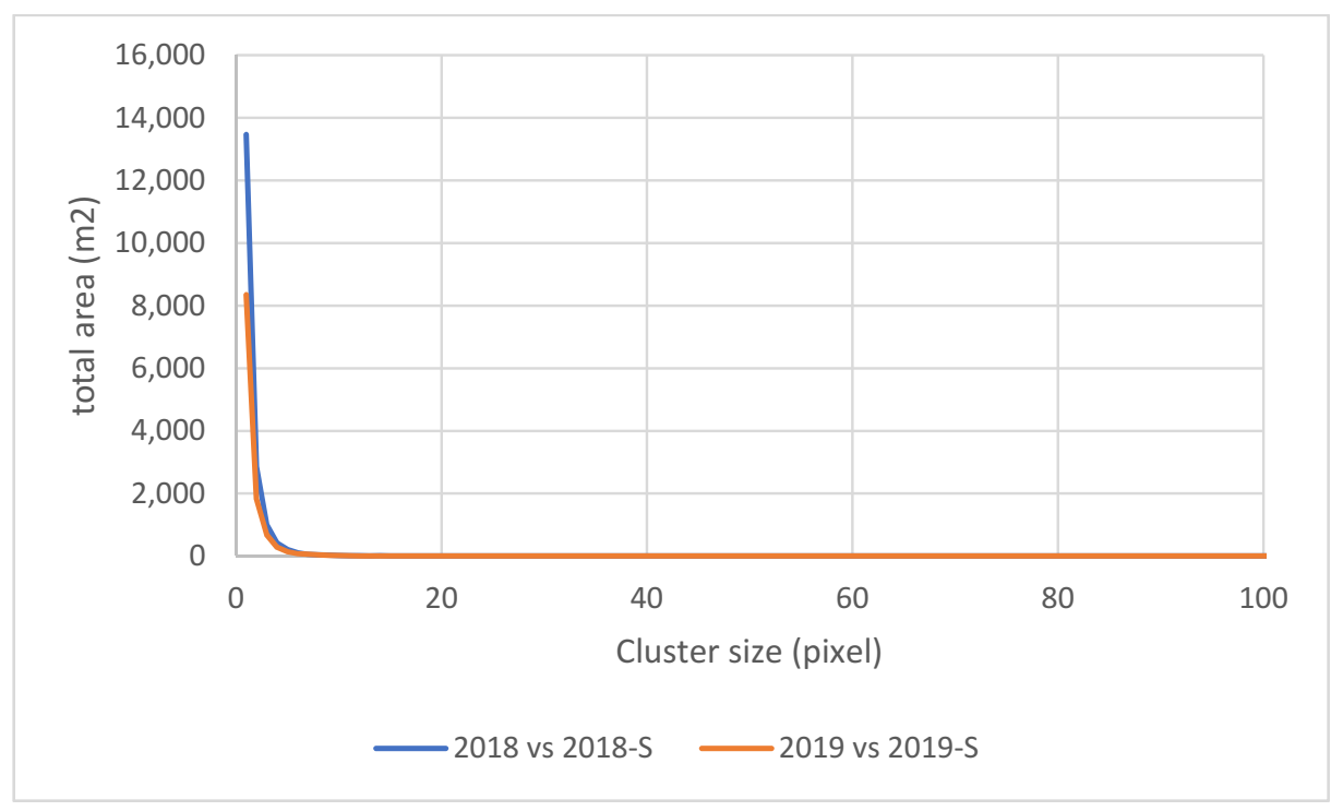
Figure 12 includes a comparison of MINDED-BA results obtained with different sensors, either exclusively (Figure 12a,e,f) or as a combination of LS8 and S2A (Figure 12b). For both 2018 and 2019, the t1 acquisitions for LS8 and S2A differ by ca. 11 days. The overlay representations of both sensors (Figure 12c,g) show an overall consistency of MINDED-BA regardless of the sensor, as demonstrated by the large majority of matching combinations. Nevertheless, regarding the mismatching combinations, we found the 2018-S and 2019-S couples to slightly underdetect LMc areas in comparison to those obtained exclusively with LS8 (particularly in 2018). In Figure 12d,h, we can verify that mismatching is mostly concentrated nearby water bodies and further away from the RBA, suggesting the occurrence of false positives for one of the datasets (based on LS8 only).

Finally, Figure 13 shows the distribution of total area of clusters of mismatching combinations obtained with the LS8 and S2A sensors, for 2018 and 2019, as previously represented in Figure 12 (2018 vs. 2018-S; and 2019 vs. 2019-S). We find the maximum total area to result from single pixel clusters (i.e., corresponding to ca. 900 m²) and to rapidly decrease with clusters size. We also verify that the total area of single pixel clusters is higher for 2018 vs. 2018-S. Such results indicate that the mismatching combinations produce salt-and-pepper noise effects, being the main source of classification inconsistency, which may contribute for the overestimation of burned areas (particularly for LS8).

4.4. Accuracy Assessment

The accuracy analysis of the MINDED-BA maps was performed with the confusion matrix approach [59].

Table 5. Confusion matrix statistics between the MINDED-BA overall burn maps results and the yearly reference burned areas (RBA) [46], from 2000 to 2019 (Nc—no change; LMc—low-magnitude change; HMc—high-magnitude change; TC—total changes (LMc+HMc); Ov—overall accuracy; TC_CE—TC commission errors; and BA_OE—burned areas omission errors).

	Accuracies (%)					Errors (%)		Total Area (ha)
	Nc	LMc	HMc	TC	Ov	TCCE	BAOE	LMc	HMc	RBA
2000	100.0	0.1	-	0.1	96.4	99.9	74.0	3645	0	8.6
2001	100.0	1.2	-	1.2	97.0	98.8	15.7	2774	0	40.1
2002	100.0	2.3	100.0	2.3	98.6	97.7	23.6	1573	0	47.6
2003	100.0	1.5	-	1.5	98.0	98.5	26.0	2232	0	45.4
2004	99.4	11.8	-	11.8	97.1	88.2	64.9	2572	0	862.0
2005	98.5	54.2	88.2	56.9	96.1	43.1	30.0	4678	403	4134.2
2006	99.7	17.2	79.3	17.2	96.9	82.8	29.6	3186	3	779.6
2007	99.9	0.6	0.0	0.6	97.5	99.4	81.9	2235	0	74.5
2008	99.9	0.9	0.0	0.9	98.3	99.1	81.7	1349	1	68.7
2009	99.9	3.5	17.1	3.6	94.6	96.4	26.7	5074	49	251.6
2010	99.6	27.6	-	27.6	98.1	72.4	42.2	1787	0	853.4
2011	99.8	4.3	-	4.3	93.8	95.7	43.5	5741	0	435.1
2012	99.8	16.9	85.0	20.3	96.9	79.7	22.9	3618	191	1003.7
2013	99.2	38.6	91.8	39.2	96.1	60.8	26.1	4329	52	2327.0
2014	100.0	0.3	0.0	0.3	96.7	99.7	43.6	3253	1	15.5
2015	99.6	20.3	-	20.3	97.7	79.7	43.6	2397	0	862.7
2016	98.9	43.3	84.6	43.6	90.6	56.4	12.7	15974	112	8033.0
2017	99.3	45.5	93.4	47.0	93.9	53.0	11.2	8897	287	4861.4
2018	100.0	0.6	100.0	0.6	96.0	99.4	9.1	4089	0	25.7
2018-S	100.0	1.1	-	1.1	98.0	98.9	13.0	2153	0	28.4
2019	99.8	25.4	-	25.4	97.0	74.6	18.1	4119	0	1276.8
2019-S	99.7	34.6	-	34.6	97.6	65.4	21.9	3749	0	1659.2
Average	99.7	16.0	61.6	16.4	96.5	83.6	34.6

and Figure 14 summarize the overall statistics, in which the distribution of both LMc and HMc classes (whose sum corresponds to the Total Changes (TC)) were analyzed in respect to the yearly reference burned areas (RBA) [46]. The quantification of such RBA (in ha) was not accounted for in masked areas or ‘Mixed’ classifications. For the purpose of summarization, we will be presenting the results of commission errors in respect to the total changes (TC_CE), i.e., false positive detections of changes, while omission errors will be presented in terms of burned areas (BA_OE), i.e., false negative cases.

The results of the confusion matrix show that MINDED-BA has a satisfactory response, reaching an average overall accuracy of 96.5%. We found Nc areas to have the highest average class accuracy (99.7%), followed by HMc (61.6%) and LMc areas (16.0%). The accuracies of HMc areas are the most variable, followed by LMc areas. In general, such variability seems to be correlated with the total area of yearly RBA, with higher LMc and HMc accuracies occurring in years with larger burned extents (e.g., for those years with over 1000 burned hectares). Regarding the 2018 and 2019 years, in Table 5 and Figure 14 we observe slightly improved accuracies for the S2A couples in comparison to LS8.

In general, we found TC_CE to be clearly higher than the BA_OE. This fact is confirmed by TC (i.e., LMc+HMc) being always higher than the RBA (Figure 14). Once again, there seems to be a correlation between RBA and error rates, with the lowest errors occurring in years with larger burned extents, particularly for TC_CE.

To verify the benefits of the multi-index approach, we repeated the confusion matrix analysis for each individual ΔBrI, with the corresponding results being summarized in

Table 6. Summary of the confusion matrix results, between every individual ΔBrI and the RBA, from 2000 to 2019 (Nc—no change; LMc—low-magnitude change; HMc—high-magnitude change; TC—total changes (LMc+HMc); Ov—overall accuracy; TC_CE—TC commission errors; and BA_OE—burned areas omission errors).

Year	ΔNBRs						ΔNBRl						ΔNBR2						ΔNDVI
	Nc	LMc	HMc	Ov	TCCE	BAOE	Nc	LMc	HMc	Ov	TCCE	BAOE	Nc	LMc	HMc	Ov	TCCE	BAOE	Nc	LMc	HMc	Ov	TCCE	BAOE
2000	100.0	0.1	0.5	92.8	99.9	41.4	100.0	0.1	-	95.7	99.9	54.7	100.0	0.1	-	99.4	99.9	93.8	100.0	0.0	-	93.8	100.0	80.5
2001	100.0	0.3	20.7	89.2	99.6	10.5	100.0	0.8	0.0	95.2	99.2	17.7	100.0	0.3	-	98.6	99.7	90.9	100.0	0.6	-	93.4	99.4	19.0
2002	100.0	0.8	-	95.4	99.2	18.0	100.0	1.7	57.1	98.0	98.3	24.2	100.0	0.6	-	97.7	99.4	72.5	100.0	0.7	32.8	96.2	98.9	25.9
2003	100.0	0.8	-	95.1	99.2	20.2	100.0	0.8	30.8	95.6	99.1	22.7	100.0	0.5	2.7	97.6	99.5	77.1	100.0	0.8	-	96.3	99.2	38.7
2004	99.4	7.9	-	93.5	92.1	50.4	99.4	8.0	55.6	94.1	92.0	54.2	99.1	3.8	-	96.1	96.2	88.0	99.3	7.4	-	95.2	92.6	68.4
2005	98.5	40.2	94.1	93.6	59.7	29.2	98.4	35.8	81.8	95.6	46.5	31.9	96.7	32.6	-	93.3	67.4	63.8	98.6	24.0	89.3	92.1	64.0	24.9
2006	99.7	9.2	78.3	93.6	90.7	27.6	99.8	4.1	63.0	91.4	92.7	25.2	99.5	7.5	0.0	94.8	92.5	56.7	99.7	15.3	-	96.7	84.7	37.9
2007	99.9	0.3	1.9	92.5	99.7	74.8	99.9	0.4	0.0	95.1	99.6	78.8	99.9	0.4	0.0	97.4	99.6	88.5	99.9	0.4	-	95.8	99.6	81.1
2008	99.9	0.5	0.5	95.2	99.5	70.7	99.9	0.7	-	97.7	99.3	81.3	99.9	0.2	-	98.1	99.8	94.8	99.9	0.7	0.0	97.2	99.3	77.0
2009	99.9	1.0	15.2	91.1	97.6	22.9	99.9	2.6	-	91.8	97.4	25.1	99.8	6.8	0.0	98.5	93.2	68.1	99.9	1.7	34.3	91.6	97.3	27.1
2010	99.6	9.9	-	93.6	90.1	34.2	99.6	19.8	-	97.1	80.2	41.2	99.1	6.4	0.0	96.5	93.6	82.5	99.5	14.0	-	96.1	86.0	44.4
2011	99.8	2.9	-	89.8	97.1	40.7	99.8	3.1	-	90.8	96.9	41.0	99.6	2.9	0.0	95.3	97.1	73.9	99.8	2.9	90.0	90.4	95.9	34.4
2012	99.8	5.0	74.9	92.4	90.5	19.8	99.8	8.9	84.6	96.1	83.0	24.0	99.3	17.4	-	98.0	82.6	73.5	99.8	9.1	-	92.3	90.9	22.5
2013	99.2	21.8	90.1	91.9	77.1	25.0	99.2	36.7	-	95.7	63.3	27.4	98.5	15.9	0.0	91.7	82.8	49.4	99.2	16.1	45.3	93.0	82.4	35.2
2014	100.0	0.1	2.4	91.3	99.9	28.5	100.0	0.2	1.3	94.4	99.8	41.5	100.0	0.1	0.0	97.1	99.9	88.1	100.0	0.2	-	94.8	99.8	46.6
2015	99.6	14.6	-	95.8	85.4	39.1	99.6	15.3	-	95.8	84.7	33.2	99.3	5.5	66.7	92.8	94.5	63.4	99.4	16.5	-	97.1	83.5	57.2
2016	98.8	10.7	58.8	86.5	66.0	12.7	98.8	41.8	91.9	90.3	57.5	14.1	97.5	70.4	44.4	95.6	29.6	30.5	98.9	32.0	0.5	85.4	68.1	11.9
2017	98.2	49.3	91.1	94.5	48.9	30.2	99.5	24.4	95.0	87.5	69.9	8.0	98.1	25.5	4.1	86.6	74.5	28.4	99.1	32.1	0.3	92.1	68.4	18.9
2018	100.0	0.4	-	93.9	99.6	12.9	100.0	0.4	27.4	95.1	99.5	10.9	100.0	0.4	-	95.4	99.6	30.6	100.0	0.3	30.5	92.4	99.5	5.7
2018-S	100.0	0.5	-	95.6	99.5	16.8	100.0	0.8	-	96.9	99.2	12.8	100.0	0.4	-	95.1	99.6	32.3	100.0	0.3	23.2	94.7	99.3	11.1
2019	99.8	20.7	-	96.2	79.3	20.0	99.8	19.6	87.8	95.8	80.1	16.5	99.6	37.9	-	98.3	62.1	29.4	99.8	15.7	95.3	94.7	74.3	10.9
2019-S	99.6	26.4	59.7	96.5	73.3	22.6	99.7	31.7	-	97.2	68.3	20.6	99.1	64.9	-	98.8	35.1	57.5	99.7	18.7	96.5	94.6	73.9	14.3
Average	99.6	10.2	45.2	93.2	88.4	30.4	99.7	11.7	52.0	94.7	86.7	32.1	99.3	13.7	10.7	96.0	86.3	65.2	99.7	9.5	44.8	93.9	89.0	36.1

. In terms of the Nc class agreement, all indexes had similar performances, with ΔNBRl and ΔNDVI having the best performances (99.7%) and ΔNBR2 the worst (99.3%). In turn, for the LMc class, ΔNBR2 achieved the highest average values (13.7%), with ΔNDVI having the lowest average agreement rate (9.5%). The results for HMc are more contrasting, with ΔNBRl showing the highest agreement levels (52.0%), while ΔNBR2 is significantly worse than the remaining ΔBrI (10.7%). Nevertheless, the best overall agreement was obtained for ΔNBR2, with an average of 96.0%, which is still under the MINDED-BA overall agreement (96.5%). In terms of errors, we can verify that the TCCE are clearly above the BAOE, confirming the tendency of overestimation of changes by every individual ΔBrI. The ΔNBR2 results have the best average TCCE (86.3%) and ΔNBRl the best average BAOE (30.4%).

Regarding the results of every individual ΔBrI in 2018 and 2019, we found slight improvements of the overall accuracies of S2A in comparison to LS8, with the exception of ΔNBR2 in 2018 and ΔNDVI in 2019.

The comparison between Table 5 and Table 6 allows us to verify that in general, MINDED-BA outperformed every ΔBrI individual parameter of the accuracy analysis, with the exception of the BA_OE, which are slightly lower for ΔNBRs and ΔNBRl.

4.5. Uncertainty Analysis

The uncertainty analysis of MINDED-BA consists in analyzing the results of the combination of the four coeval ΔBrI thematic maps. For this procedure, we defined a range of uncertainty classes, ranging from 0 to 3:

0—unanimity (four identical coeval classifications)

1—absolute majority (with three identical coeval classifications)

2—relative majority (with two identical coeval classifications)

3—no majority (tie between two couples of identical coeval classifications).

The above mentioned pixel-scale values allowed us to obtain the overall uncertainty, which corresponds to the uncertainty class values weighted according to their frequency.

Table 7. Uncertainty class distribution of yearly overall MINDED-BA results.

Years	Uncertainty Classes
	0		1		2		3
	Area (ha)	%	Area (ha)	%	Area (ha)	%	Area (ha)	%	Overall Uncertainty
2000	948,900	91.0	73,613	7.1	158	0.0	20,162	1.9	0.13
2001	823,368	85.8	105,364	11.0	153	0.0	30,975	3.2	0.21
2002	1,049,771	92.0	76,194	6.7	0	0.0	15,516	1.4	0.11
2003	1,050,957	91.3	73,423	6.4	13	0.0	26,504	2.3	0.13
2004	896,207	88.9	84,347	8.4	7	0.0	27,907	2.8	0.17
2005	778,087	85.9	91,987	10.2	8282	0.9	27,052	3.0	0.21
2006	857,233	87.7	80,862	8.3	848	0.1	38,361	3.9	0.20
2007	832,291	89.3	73,488	7.9	86	0.0	25,883	2.8	0.16
2008	793,570	93.4	43,421	5.1	2277	0.3	10,562	1.2	0.09
2009	837,502	87.3	84,842	8.8	7194	0.7	30,194	3.1	0.20
2010	813,525	90.1	71,555	7.9	17	0.0	17,348	1.9	0.14
2011	795,139	83.6	122,965	12.9	0	0.0	33,116	3.5	0.23
2012	934,072	87.8	97,178	9.1	3373	0.3	28,721	2.7	0.18
2013	718,831	84.8	105,790	12.5	3093	0.4	19,652	2.3	0.20
2014	893,693	88.3	87,313	8.6	2061	0.2	29,480	2.9	0.18
2015	898,133	89.7	83,251	8.3	0	0.0	19,340	1.9	0.14
2016	866,092	78.1	174,932	15.8	32,917	3.0	35,384	3.2	0.31
2017	722,058	77.7	156,027	16.8	1843	0.2	49,610	5.3	0.33
2018	1,033,961	87.4	126,319	10.7	106	0.0	22,158	1.9	0.16
2018-S	981,285	88.8	103,376	9.4	2	0.0	20,231	1.8	0.15
2019	1,175,889	94.5	53,367	4.3	137	0.0	14,887	1.2	0.08
2019-S	1,092,660	93.5	65,780	5.6	3	0.0	9662	0.8	0.08

summarizes the results of the uncertainty analysis, where we can verify that MINDED-BA uncertainty values are mostly 0 and 1, which contribute to low overall uncertainties. However, for every year, the highest uncertainty class (i.e., 3) exceeds the intermediate class (i.e., 2). From the entire dataset, we found that both 2019 and 2019-S have the lowest average uncertainties, while 2017, 2016, and 2011 have the highest average uncertainties.

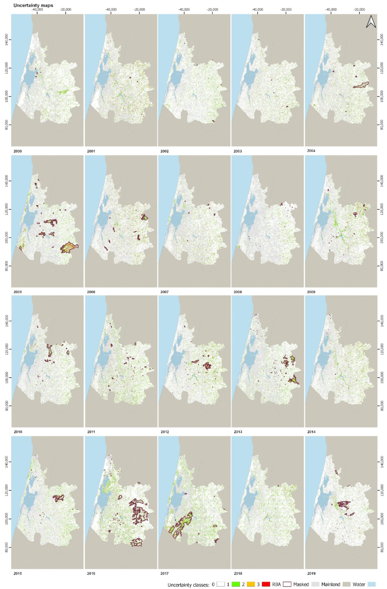
Figure 15 shows the uncertainty maps for MINDED-BA, where we can observe that the highest uncertainty classes (i.e., 2 and 3) tend to be located within the limits of RBA. Pixels corresponding to uncertainty values of 1 seem to be either randomly distributed (e.g., 2003, 2010) or concentrated nearby water bodies (along the lower sections of the Vouga River and around the Pateira de Fermentelos lagoon, e.g., for 2000, 2001, 2009, 2014, and 2019).

5. Discussion

This study presents a change detection model for determining burned extents from wildfires. It consists of the development of a previous model (MINDED), originally designed for determining flood extents [34]. Despite both being weather-related hazards [60,61], flooding and wildfires have antagonistic causes and effects. Floods are often the consequence of extreme precipitation events, while wildfires tend to occur and proliferate during dry periods. Nonetheless, this work demonstrates that the same theoretical principles can be applied to determine the extents of both hazardous processes. This can be done by selecting different hazard-specific indices or by focusing on different sides of the same index difference distribution curves. Since MINDED and MINDED-BA share the same theoretical principles, they also share certain advantages and limitations. By combining several indices based on different multispectral regions, both methods allow narrowing the range of types of change, in which burned area detection is also included.

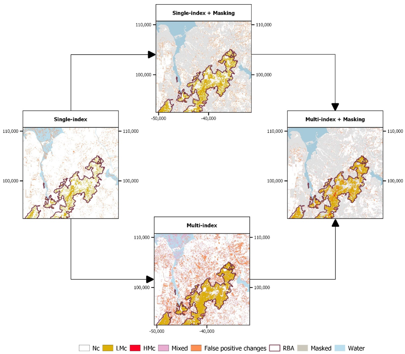
When analyzing processes such as wildfires, which have non-Boolean characteristics and result from interaction with other natural and anthropic processes, it is essential to define an adequate set of procedures to ensure the quality of the modelled results. Figure 16 highlights both the advantages of the multi-index approach (Multi-index) and the importance of the pre-processing developments (Masking) introduced in MINDED-BA, in that the final result shows clear improvements when compared to the reference burned areas (RBA) [46]. Nevertheless, as an index-differencing-based approach, it is still not completely able to discriminate each type of change.

As a digital change detection method, MINDED-BA is intrinsically dependent on the quality and quantity of the information conveyed by the images used for both t0 and t1 scenes. This means that the choice of the time of acquisition and frequency of the image couples should take into consideration the purpose of the research, as well as the geographical location and the characteristics of the study area. In our case, for the estimation of yearly burned areas in temperate Mediterranean climate regions, t0 and t1 should be acquired as close as possible to the end of each year, to ensure that each forest fire season has ended. Considering MINDED-BA relies on multispectral images acquired by sensors with revisiting periods of several days, such as those provided by Landsat or Sentinel-2, this might present additional difficulties. The first difficulty is to find cloud-free images during the wet season, which for particularly rainy years may be hard to obtain, especially for older epochs with a more limited scene availability. For this reason, it was not possible to select images acquired exactly at the same time of every year, ranging from late September to late January of the following year. This may be considered as an important source of error, since more changes other than burning may become detected by MINDED-BA (e.g., phenological cycles, seasonal agricultural or forestry management practices). On the other hand, the selection of only one couple of images per year may prevent detecting changes in recurring fires taking place in the same location within less than a one-year interval (e.g., in areas experiencing fast vegetation regrowth). Additionally, due to such limited image availability and the total time extent of this study (i.e., 19 years), we had to consider couples of images acquired by different sensors (Table 2). Nevertheless, as referred to by [34], we verified that using different sensors for t0 and t1 does not affect the accuracy of the model significantly, while causing a shift of the ΔBrI modal values and, consequently, of the threshold values (as observed in Table A3 and Figure 8). As verified in Figure 11, no major inconsistencies were found when comparing results obtained from relatively concomitant Landsat 8 or Sentinel-2A scenes. This fact confirms the robustness of the model workflow (Figure 1), which performed similarly in detecting burned areas (compared to the RBA). Nevertheless, the few differences highlighted in Table 3 and Figure 11c,d,g,h and Figure 13 are more likely resultant from local water-content-related changes occurring during the ca. 11 days separating the t1 scenes acquired by each sensor. In fact, another difficulty for MINDED-BA is that several phenomena other than fires may constitute false positives for every ΔBrI, which may only be mitigated with further pre-processing steps.

Regarding the atmospheric correction of the multispectral images used as t0 and t1, to ensure the replicability and robustness of MINDED-BA results, we considered the Level-2 products of both Landsat and Sentinel-2 (i.e., given as surface reflectance), which are determined by the USGS and ESA algorithms [41,62,63,64]. For the same reasons, we also considered the quality assessment bands (‘pixel_qa’ and SCL, respectively), which were used to mask clouds, cloud shadows, water, and snow features. Nevertheless, considering the relative stability of permanent water bodies within our study area and the ready availability of spatial thematic data containing their limits, we defined a buffer area with the objective of masking such permanent water bodies. This ensured that none of those pixels remained undetected by the Level-2 algorithms and avoided any further interference with the MINDED-BA results.

Additional criteria are also necessary to discard other known potential interferences such as forest/shrubland clearcutting, agricultural crop harvesting, or soil mobilization occurring between t0 and t1. This might be achieved with pre- or post-processing masking of highly reflective surfaces (HRS), which might occur in t1, resulting in false positive detections. Such a task may be implemented by creating a user-defined training dataset or by considering reference literature values. The first option has the advantage of providing the best correlation with the characteristics of a study area, but may require a priori knowledge of both bare soil and burned area locations (e.g., using analogous approaches to [35]), being more dependent on the end-user expertise and technical skills. On the other hand, classifications based on reference land cover literature values allow for implementing the model in a fully automatic routine without any subjectivity issues. The latter also has the potential of being applied as a ‘black-box’ tool, targeted for non-experts in remote sensing techniques. Since the thresholding procedures of MINDED-BA rely entirely on the index differencing statistics, there is a clear advantage in implementing masking as a pre-processing step (as opposed to post-processing), because by eliminating such interferences, the signal separation between changes and no-changes is also improved (i.e., noise reduction). For these reasons, we adopted a theoretical reference value approach to define a thresholding range applied to those multispectral bands that maximize the separation between burned areas and HRS. Then, we determined sensor-specific Tasseled Cap Brightness (TCB) values for a series of increments within the thresholding range, which were later used to mask HRS from every t1 scene. In principle, we expected the best masking to correspond to those increments positioned towards the middle of the thresholding range, as their position was likely to maximize the difference towards the HRS theoretical reflectance signatures and to provide the best trade-off between the Total Changes commission errors (TC_CE) and the Burned Areas omission errors (BA_OE). In fact, if MINDED-BA was to be applied without any complementary information or additional analysis, M2 or M3 would likely be the safest alternatives. Instead, we found that the lowest threshold (i.e., M1) was the best option for our case study (see Figure 4). This result may be explained by the different spectral characteristics of the burned areas, as well as the reflectivity of HRS due to local pedology and geology. Moreover, we would like to highlight that instead of the TCB, we could have directly integrated the same multispectral bands, as sum or average of reflectance values. After trying such approaches, we verified that despite having similar results, the TCB provided slightly better masking of HRS, obtaining marginal but consistent improvements (ca. 1%) for every parameter of the confusion matrix.

The optimal bin selection approach introduced in this work is a further development to the MINDED threshold selection procedure. It consists of a conceptual interpretation of the shape for the ΔBrI frequency distribution function, depicting what are the expected indications caused by noise and signal variations. Despite the different ΔBrI under analysis being obtained by integrating different multispectral band combinations and the tested bin number values being characterized by a set of 15 samples in a quite large range (10–1259), the obtained range of optimal bin numbers is concentrated in only 3 samples (i.e., 28, 40, 56-see Figure 6). These findings may be a consequence of the effects of the time span between t0 and t1 images, as well as the extent and type of changes. However, further research should be performed to truly understand this behavior. As for the thresholds T1 and T2, in theory these should fall within the range of ΔBrI values 0–2 (as only normalized indices were considered). The results show that T1 is more concentrated in a small range of values (interquartile range 0.10–0.36), while a wider range characterizes T2 (0.45–0.99). We can conclude that the optimal bin number distribution spreads within ca. 20% of the sampled range, while the threshold T1 spreads within ca. 13% of the expected range, hence suggesting high stability regardless of the ΔBrI. On the other hand, T2 spreads within ca. 27%, suggesting higher variability.

Regarding the threshold distribution, there are several factors affecting their magnitude and variability. Such factors include the types of changes occurring between t0 and t1, as well as the sensors used to detect them, which in some cases are different between the two epochs (Table 2). For these reasons, such threshold variations should not be interpreted as an indicator of uncertainty, as they reflect the method’s response to a shift of the modal value of the frequency distribution functions. The higher variability observed for T2 should also be more dependent on the optimal bin number value, because the higher the bin number, more intermediate thresholds may be detected (Figure 7).

If not addressed correctly, or addressed at all, some of the above-mentioned conditions may still produce effects over the entire MINDED-BA model chain. In those cases, the ΔBrI distribution functions and their corresponding d1f and d2f may be affected, triggering the possibility of detecting sub-optimal thresholds and leading to less accurate classification as burn-related changes (either as LMc or HMc). Despite all the pre-processing steps, MINDED-BA seems to have a tendency of overestimating burned areas in comparison to the RBA (as observed in Figure 10, Figure 11 and Figure 14 and Table 5). This tendency is likely a consequence of the wide and flat topography of the lower section of the Vouga River Watershed. In some cases, we found several LMc areas to occur nearby river bodies that are prone to flooding [34] (e.g., for 2000, 2009, 2014, and 2018). Moreover, MINDED-BA may be also sensitive to either higher differentials of vegetation greenness or water contents between t0 and t1 images, as might be the case for 2013 and 2016. This means that in such cases, t0 was probably acquired during particularly wetter or even flooded conditions and/or t1 during a drought. Both these conditions were observed for 2016 (see Figure 11), especially for t1, which was acquired during a well-documented drought period [65,66]. As an alternative, both t0 and t1 scenes could have been acquired earlier than the wet season, but with the risk of missing burned areas from those years.

From the initial set of normalized indices, we found ΔNDWI results to have insufficient performances in detecting burned areas (Figure 9), so we discarded it from further steps of MINDED-BA. For these reasons, we ended up using four ΔBrI. In general, we found ΔNBRl to have the best individual performance for most parameters of the confusion matrix analysis, while ΔNBR2 achieved the best overall accuracy with the RBA (Table 6). These findings confirm the indications found in the literature [18,28], which highlight the benefits of considering both SWIRs and SWIRl to improve the discrimination between burned areas and water. However, as observed in the examples of Figure 9, ΔNBR2 seems to underestimate certain burned areas, probably resulting from reduced fire severity conditions. The majority analysis of MINDED-BA has been demonstrated to handle most individual ΔBrI limitations, meaning that the overall maps of Figure 10 represent the best combination for most of the confusion matrix parameters (Table 5). Moreover, the uncertainty assessment, which is enabled by the majority analysis, provides additional and relevant information about those locations where MINDED-BA tends to perform with different levels of confidence.

The analysis of the confusion matrix along with the RBA extents indicates that, in general, the larger the burned areas, the better the performance of the MINDED-BA. This is likely the consequence of MINDED-BA being a statistically dependent method, requiring that the frequency of pixels corresponding to burn-related changes should be large enough to produce measurable changes to df1 and df2 functions (though not enough to become the majority). Nevertheless, the method accuracy is also dependent on the occurrence of other types of changes that may lead to detecting false positives, such as those verified in 2016.

Despite being the widest within our study area, wildfires are not exclusive to forests or agricultural areas. In particular, during those years with the largest burned areas, many fires involved other land covers, such as artificial or even wetland areas (e.g., for 2017). Such heterogeneity of burned surfaces increases the difficulty in finding optimal thresholds, which ideally would have to be transversal to detect burn-related changes for every type of land cover.

Regarding the ICNF official burned areas, which were used as our RBA, they are the closest available dataset that may be used as a ground truth alternative. However, this dataset is in practice a product of a multi-source survey, combining fieldwork and remote sensing data interpretation. This means that these are also affected by unknown errors that, as an example, may overestimate the real extent of burned areas (e.g., as seen in Figure 4, where the outer RBA polygon seems to be including several non-burned islands) and consequently increase the BA_OE. Additionally, this ICNF dataset is mostly Boolean in terms of the occurrence of fires; therefore, we have no way of verifying which fire severities are being considered. Nevertheless, in recent years, ICNF has started releasing additional information, such as date, type of fire (e.g., shrubland, agriculture, and forestry), cause of ignition, or source, which seem to demonstrate coordination with multi-level civil protection agents.

The tendency towards overestimating is a common issue for any image-differencing method based on a bi-temporal analysis, particularly when implemented with couples of images with one year or larger temporal separation. However, since MINDED-BA has been completely integrated in an automatic script, it should be relatively easy to implement it in a systematic routine, in order to analyze different couples of images acquired within a shorter time span (i.e., corresponding to the satellite temporal resolution). This would also enable assessing the yearly burned areas’ extents. In fact, if such analysis was to be performed, the user subjectivity errors when selecting the images would no longer persist, and the overestimation issue should be highly minimized. Such higher frequency multitemporal comparisons would also allow analyzing the persistence (or not) of detected changes across more than a couple of images, which by itself should allow a systematic improvement of burned-extent detection. Finally, considering that MINDED-BA has been demonstrated to be implemented automatically with readily available multispectral satellite data, it may be useful in both regional- and national-level applications. However, when analyzing considerably larger areas, it would be advisable to split the implementation of MINDED-BA by using images acquired along the same orbital path. Any further extents could be joined later as post-classification results, minimizing any potential interferences resulting from different t1 acquisition dates.

6. Conclusions

This paper presents MINDED-BA, an automatic change detection method based on multispectral optical satellite images, aimed at determining yearly burned extents. The method was implemented within a study area located in northwest central Portugal, using Landsat and Sentinel-2 data from 2000 to 2019. This work is the development of a previous multi-index differencing method, originally designed to detect flood extents. MINDED-BA allows detecting burn-related changes, based on the analysis of magnitudes of the image-differencing statistics. Another relevant aspect of the method concerns the development and implementation of several pre-processing steps introduced within the modelling workflow, with the objective of discarding some of the most significant sources of error mentioned in the literature. From such developments, we highlight a new procedure to mask highly reflective surfaces, based on land-cover-specific multispectral literature reflectance values, which were integrated and implemented in MINDED-BA through tasseled cap brightness values. Moreover, the optimal bin number selection procedure introduced in this work to process the image-differencing statistics, which is the basis for the threshold selection for the classification of changes, has been demonstrated to be a consistent and subjectivity-free approach. The performance of such innovations was verified by comparing MINDED-BA outputs with an official dataset of burned areas. Moreover, MINDED-BA also showed significant improvements compared to the single-index results. In fact, its majority analysis allowed combining the classifications provided by the best performing indices, while reducing noise caused by single-index false positives. Nevertheless, in comparison to the reference burned extents, MINDED-BA tends to overestimate burned areas, being sensitive to changes other than those from burning. This was particularly noticeable whenever the couples of images used to perform index differencing were acquired under significantly changed conditions over about one year (e.g., in terms of water content, seasonal vegetation greenness, or when major land-use changes take place).

The method was implemented through an automatic Python script, selecting one multispectral scene per year, acquired after the study area annual fire season. Considering the ease of implementation provided by a GRASSGIS Python script, its straightforward theoretical principles, and its effective results, MINDED-BA has the potential of being useful as a reliable unsupervised method for the preliminary assessment of regional- and national-level yearly burned extents. Moreover, considering the equivalent performance among the different tested sensors (i.e., Landsat 5–8 and Sentinel-2A), it allows increasing the temporal resolution of input data, which may contribute to mitigating detection errors.

References

- Chuvieco, E.; Aguado, I.; Jurdao, S.; Pettinari, M.L.; Yebra, M.; Salas, J.; Hantson, S.; de la Riva, J.; Ibarra, P.; Rodrigues, M.; et al. Integrating geospatial information into fire risk assessment. Int. J. Wildland Fire 2014, 23, 606–619. [Google Scholar] [CrossRef]
- Abdollahi, M.; Islam, T.; Gupta, A.; Hassan, Q.K. An advanced forest fire danger forecasting system: Integration of remote sensing and historical sources of ignition data. Remote Sens. 2018, 10, 923. [Google Scholar] [CrossRef] [Green Version]
- Leblon, B.; San-Miguel-Ayanz, J.; Bourgeau-Chavez, L.; Kong, M. Remote Sensing of Wildfires. In Land Surface Remote Sensing: Environment and Risks; Baghdadi, N., Zribi, M., Eds.; Elsevier: Amsterdam, The Netherlands, 2016; pp. 55–95. ISBN 9780081012659. [Google Scholar]
- Bajocco, S.; Guglietta, D.; Ricotta, C. Modelling fire occurrence at regional scale: Does vegetation phenology matter? Eur. J. Remote Sens. 2015, 48, 763–775. [Google Scholar] [CrossRef] [Green Version]
- Chuvieco, E.; Aguado, I.; Yebra, M.; Nieto, H.; Salas, J.; Martín, M.P.; Vilar, L.; Martínez, J.; Martín, S.; Ibarra, P.; et al. Development of a framework for fire risk assessment using remote sensing and geographic information system technologies. Ecol. Modell. 2010, 221, 46–58. [Google Scholar] [CrossRef]
- Aguado, I.; Chuvieco, E.; Nieto, H. Estimation of dead fuel moisture content from meteorological data in Mediterranean areas. Int. J. Wildland Fire 2007, 16, 390–397. [Google Scholar] [CrossRef]
- Liu, B.; Siu, Y.L.; Mitchell, G. Hazard interaction analysis for multi-hazard risk assessment: A systematic classification based on hazard-forming environment. Nat. Hazards Earth Syst. Sci. 2016, 16, 629–642. [Google Scholar] [CrossRef] [Green Version]
- Adab, H.; Kanniah, K.D.; Solaimani, K.; Sallehuddin, R. Modelling static fire hazard in a semi-arid region using frequency analysis. Int. J. Wildland Fire 2015, 24, 763–777. [Google Scholar] [CrossRef]
- Matin, M.A.; Chitale, V.S.; Murthy, M.S.R.; Uddin, K.; Bajracharya, B.; Pradhan, S. Understanding forest fire patterns and risk in Nepal using remote sensing, geographic information system and historical fire data. Int. J. Wildland Fire 2017, 26, 276. [Google Scholar] [CrossRef] [Green Version]
- Schroeder, W.; Oliva, P.; Giglio, L.; Quayle, B.; Lorenz, E.; Morelli, F. Active fire detection using Landsat-8/OLI data. Remote Sens. Environ. 2016, 185, 210–220. [Google Scholar] [CrossRef] [Green Version]
- Vilar, L.; Camia, A.; San-Miguel-Ayanz, J. A comparison of remote sensing products and forest fire statistics for improving fire information in mediterranean Europe. Eur. J. Remote Sens. 2015, 48, 345–364. [Google Scholar] [CrossRef] [Green Version]
- Kavzoglu, T.; Erdemir, M.Y.; Tonbul, H. Evaluating performances of spectral indices for burned area mapping using object-based image analysis. In Proceedings of Spatial Accuracy 2016; Gebze Technical University, Department of Geomatics Engineering: Kocaeli, Turkey, 2014; pp. 1–7. [Google Scholar]
- Chuvieco, E.; Riaño, D.; Aguado, I.; Cocero, D. Estimation of fuel moisture content from multitemporal analysis of Landsat Thematic Mapper reflectance data: Applications in fire danger assessment. Int. J. Remote Sens. 2002, 23, 2145–2162. [Google Scholar] [CrossRef]
- Verde, J.C.; Zêzere, J.L. Assessment and validation of wildfire susceptibility and hazard in Portugal. Nat. Hazards Earth Syst. Sci. 2010, 10, 485–497. [Google Scholar] [CrossRef]
- Parente, J.; Pereira, M.G. Structural fire risk: The case of Portugal. Sci. Total Environ. 2016, 573, 883–893. [Google Scholar] [CrossRef]
- Keeley, J.E. Fire intensity, fire severity and burn severity: A brief review and suggested usage. Int. J. Wildland Fire 2009, 18, 116–126. [Google Scholar] [CrossRef]
- Leuenberger, M.; Parente, J.; Tonini, M.; Pereira, M.G.; Kanevski, M. Wildfire susceptibility mapping: Deterministic vs. stochastic approaches. Environ. Model. Softw. 2018, 101, 194–203. [Google Scholar] [CrossRef]
- Bastarrika, A.; Chuvieco, E.; Martín, M.P. Mapping burned areas from landsat TM/ETM+ data with a two-phase algorithm: Balancing omission and commission errors. Remote Sens. Environ. 2011, 115, 1003–1012. [Google Scholar] [CrossRef]
- Rouse, J.W.; Hass, R.H.; Schell, J.A.; Deering, D.W. Monitoring vegetation systems in the great plains with ERTS. Third Earth Resour. Technol. Satell. Symp. 1973, 1, 309–317. [Google Scholar]
- Satir, O.; Berberoglu, S.; Donmez, C. Mapping regional forest fire probability using artificial neural network model in a Mediterranean forest ecosystem. Geomat. Nat. Hazards Risk 2016, 7, 1645–1658. [Google Scholar] [CrossRef] [Green Version]
- McFeeters, S.K. The use of the Normalized Difference Water Index (NDWI) in the delineation of open water features. Int. J. Remote Sens. 1996, 17, 1425–1432. [Google Scholar] [CrossRef]
- Key, C.H.; Benson, N.C. Measuring and remote sensing of burn severity [poster abstract]. Jt. Fire Sci. Conf. Work. Proc. 1999, II, 284–285. [Google Scholar]
- Trigg, S.; Flasse, S. An evaluation of different bi-spectral spaces for discriminating burned shrub-savannah. Int. J. Remote Sens. 2001, 22, 2641–2647. [Google Scholar] [CrossRef]
- USGS Landsat Normalized Burn Ratio 2. Available online: https://www.usgs.gov/core-science-systems/nli/landsat/landsat-normalized-burn-ratio-2 (accessed on 12 December 2021).
- Escuin, S.; Navarro, R.; Fernández, P. Fire severity assessment by using NBR (Normalized Burn Ratio) and NDVI (Normalized Difference Vegetation Index) derived from LANDSAT TM/ETM images. Int. J. Remote Sens. 2008, 29, 1053–1073. [Google Scholar] [CrossRef]
- Sahana, M.; Ganaie, T.A. GIS-based landscape vulnerability assessment to forest fire susceptibility of Rudraprayag district, Uttarakhand, India. Environ. Earth Sci. 2017, 76, 676. [Google Scholar] [CrossRef]
- Parker, B.M.; Lewis, T.; Srivastava, S.K. Estimation and evaluation of multi-decadal fire severity patterns using Landsat sensors. Remote Sens. Environ. 2015, 170, 340–349. [Google Scholar] [CrossRef]
- Pereira, J.M.C.; Sá, A.C.L.; Sousa, A.M.O.; Silva, J.M.N.; Santos, T.N.; Carreiras, J.M.B. Remote Sensing of Large Wildfires. In Remote Sensing of Large Wildfires; Chuvieco, E., Ed.; Springer: Berlin/Heidelberg, Germany, 1999; ISBN 9783642601644. [Google Scholar]
- Chuvieco, E.; Martín, M.P.; Palacios, A. Assessment of different spectral indices in the red-near-infrared spectral domain for burned land discrimination. Int. J. Remote Sens. 2002, 23, 5103–5110. [Google Scholar] [CrossRef]
- Martín, M.P.; Gómez, I.; Chuvieco, E. Burnt Area Index (BAIM) for burned area discrimination at regional scale using MODIS data. For. Ecol. Manag. 2006, 234, S221. [Google Scholar] [CrossRef]
- Lillesand, T.M.; Kiefer, R.W.; Chipman, J.W. Remote Sensing and Image Interpretation, 7th ed.; John Wiley and Sons, Wiley: Hoboken, NJ, USA, 2015; ISBN 978-1-118-34328-9. [Google Scholar]
- Singh, A. Review Article: Digital change detection techniques using remotely-sensed data. Int. J. Remote Sens. 1989, 10, 989–1003. [Google Scholar] [CrossRef] [Green Version]
- Campbell, J.B.; Wynne, R.H. Introduction to Remote Sensing, 5th ed.; The Guilford Press: New York, NY, USA, 2011; ISBN 978-1-60918-176-5. [Google Scholar]
- Oliveira, E.R.; Disperati, L.; Cenci, L.; Pereira, L.G.; Alves, F.L. Multi-Index Image Differencing Method (MINDED) for flood extent estimations. Remote Sens. 2019, 11, 1305. [Google Scholar] [CrossRef] [Green Version]
- Cenci, L.; Disperati, L.; Persichillo, M.G.; Oliveira, E.R.; Alves, F.L.; Phillips, M. Integrating remote sensing and GIS techniques for monitoring and modeling shoreline evolution to support coastal risk management. GIScience Remote Sens. 2017, 55, 355–375. [Google Scholar] [CrossRef]
- de Luca, G.; Silva, J.M.N.; Modica, G. A workflow based on Sentinel-1 SAR data and open-source algorithms for unsupervised burned area detection in Mediterranean ecosystems. GIScience Remote Sens. 2021, 58, 516–541. [Google Scholar] [CrossRef]
- Ma, Z.; Xie, Y.; Jiao, J.; Li, L.; Wang, X. Study on the relationship between scirpus planiculmis grow and Soil water content. Procedia Environ. Sci. 2011, 10, 2029–2035. [Google Scholar] [CrossRef] [Green Version]
- EEA. Mapping the Impacts of Recent Natural Disasters and Technological Accidents in Europe—An Overview of the Last Decade; EEA: Copenhagen, Denmark, 2010. [Google Scholar]
- Song, C.; Woodcock, C.E.; Seto, K.C.; Lenney, M.P.; Macomber, S.A. Classification and change detection using Landsat TM data: When and how to correct atmospheric effects? Remote Sens. Environ. 2001, 75, 230–244. [Google Scholar] [CrossRef]
- U.S. Geological Survey. Landsat 8 Surface Reflectance Code (LASRC) Poduct Guide. (No. LSDS-1368 Version 2.0); EROS: Sioux Falls, SD, USA, 2019. [Google Scholar]
- Ihlen, V. USGS Landsat 7 (L7) Data Users Handbook. USGS Landsat User Serv. 2019, 7, 151. [Google Scholar]
- Zhu, Z.; Woodcock, C.E. Remote Sensing of Environment Object-based cloud and cloud shadow detection in Landsat imagery. Remote Sens. Environ. 2012, 118, 83–94. [Google Scholar] [CrossRef]
- Hughes, M.J.; Hayes, D. Automated Detection of Cloud and Cloud Shadow in Single-Date Landsat Imagery Using Neural Networks and Spatial Post-Processing. Remote Sens. 2014, 4907–4926. [Google Scholar] [CrossRef] [Green Version]
- Hantson, S.; Chuvieco, E. Evaluation of different topographic correction methods for landsat imagery. Int. J. Appl. Earth Obs. Geoinf. 2011, 13, 691–700. [Google Scholar] [CrossRef]
- Schowengerdt, R.A. Remote Sensing: Models and Methods for Image Processing, 3rd ed.; Academic Press: Burlington, VT, USA, 2007; ISBN 9780123694072. [Google Scholar]
- ICNF Cartografia de Áreas Ardidas. Available online: http://www2.icnf.pt/portal/florestas/dfci/inc/mapas (accessed on 12 December 2021).
- Coelho, C.O.A.; Alves, F.L.; Ferreira, A.; Castanheira, E.; Esteves, T.C. Relatório Final Risco de Incêndio Florestal; Definição das condições de risco de cheia, incêndios florestais, erosão costeira e industriais na área de intervenção da AMRIA; AMRIA: Aveiro, Portugal, 2007. [Google Scholar]
- ICNF. Programa Regional de Ordenamento Florestal-Centro Litoral. Caracterização Biofísica, Socioeconómica e Dos Recursos Florestais; ICNF: Lisbon, Portugal, 2019. [Google Scholar]
- USGS Earth Explorer. Available online: https://earthexplorer.usgs.gov/ (accessed on 12 November 2020).
- ESA Copernicus Open Access Hub. Available online: https://scihub.copernicus.eu/dhus/ (accessed on 11 December 2020).
- U.S. Geological Survey. Landsat 4–7 Surface Reflectance (Ledaps) Product Guide; EROS: Sioux Falls, SD, USA, 2019. [Google Scholar]
- DGT SNIG-Sistema Nacional de Informação Geográfica. Available online: https://snig.dgterritorio.gov.pt/ (accessed on 12 December 2021).
- Riaño, D.; Chuvieco, E.; Salas, J.; Aguado, I. Assessment of different topographic corrections in landsat-TM data for mapping vegetation types (2003). IEEE Trans. Geosci. Remote Sens. 2003, 41, 1056–1061. [Google Scholar] [CrossRef] [Green Version]
- JAXA ALOS Global Digital Surface Model “ALOS World 3D-30 m (AW3D30)”. Available online: https://www.eorc.jaxa.jp/ALOS/en/aw3d30/index.htm (accessed on 12 November 2020).
- Runge, A.; Grosse, G. Comparing spectral characteristics of Landsat-8 and Sentinel-2 same-day data for arctic-boreal regions. Remote Sens. 2019, 11, 1730. [Google Scholar] [CrossRef] [Green Version]
- Mancino, G.; Ferrara, A.; Padula, A.; Nolè, A. Cross-Comparison between Landsat 8 (OLI) and Landsat 7 (ETM+) Derived Vegetation Indices in a Mediterranean Environment. Remote Sens. 2020, 12, 291. [Google Scholar] [CrossRef] [Green Version]
- Chander, G.; Hewison, T.J.; Fox, N.; Wu, X.; Xiong, X.; Blackwell, W.J. Overview of intercalibration of satellite instruments. IEEE Trans. Geosci. Remote Sens. 2013, 51, 1056–1080. [Google Scholar] [CrossRef]
- EEA Corine Land Cover (CLC) 2012. Available online: https://land.copernicus.eu/pan-european/corine-land-cover/clc-2012 (accessed on 12 December 2021).
- Congalton, R.G. A review of assessing the accuracy of classifications of remotely sensed data. Remote Sens. Environ. 1991, 37, 35–46. [Google Scholar] [CrossRef]
- Lavalle, C.; Barredo, J.I.; De Roo, A.; Niemeyer, S.; San Miguel-Ayanz, J.; Genovese, E.; Camia, A. Towards an European Integrated Map of Risk from Weather Driven Events; JRC: Brussels, Belgium, 2005. [Google Scholar]
- Deleu, J.; Tambuyzer, H.; Stephenne, N. Multi Risk preparedness supported by Earth Observation. In Proceedings of the Eurosense Gi4DM Conference, Antalaya, Turkey, 3–8 May 2011. [Google Scholar]
- U.S. Geological Survey. Landsat 8 Data Users Handbook; EROS: Sioux Falls, SD, USA, 2016; p. 106. [Google Scholar]
- Thales Alenia Space. Sentinel-2 Products Specification Document; Thales Alenia Space: Cannes, France, 2021. [Google Scholar]
- SUHET. Sentinel-2 User Handbook; ESA: Paris, France, 2015; Volume 2. [Google Scholar]
- APA Environmental Risks-Drought. Available online: https://rea.apambiente.pt/content/drought?language=en (accessed on 7 December 2021).
- García-Herrera, R.; Garrido-Perez, J.M.; Barriopedro, D.; Ordóñez, C.; Vicente-Serrano, S.M.; Nieto, R.; Gimeno, L.; Sorí, R.; Yiou, P. The European 2016/17 drought. J. Clim. 2019, 32, 3169–3187. [Google Scholar] [CrossRef]
- Crist, E.P. A TM Tasseled Cap equivalent transformation for reflectance factor data. Remote Sens. Environ. 1985, 17, 301–306. [Google Scholar] [CrossRef]
- Huang, C.; Yang, W.L.; Homer, C.; Zylstra, G.; Huang, C.; Yang, W.L.; Wylie, B.; Yang, L.; Homer, C. Derivation of a tasselled cap transformation based on Landsat 7 at-satellite reflectance Derivation of a tasselled cap transformation based on Landsat 7 at-satellite re ectance. Int. J. Remote Sens. 2002, 23, 1741–1748. [Google Scholar] [CrossRef]
- Baig, M.H.A.; Zhang, L.; Shuai, T.; Tong, Q. Derivation of a tasselled cap transformation based on Landsat 8 at-satellite reflectance. Remote Sens. Lett. 2014, 5, 423–431. [Google Scholar] [CrossRef]
- Shi, T.; Xu, H. Derivation of Tasseled Cap Transformation Coefficients for Sentinel-2 MSI At-Sensor Reflectance Data. IEEE J. Sel. Top. Appl. Earth Obs. Remote Sens. 2019, 12, 4038–4048. [Google Scholar] [CrossRef]
Figure 1.
The Multi-Index Differencing method for Burned Areas (MINDED-BA) workflow (adapted from [34]).
Figure 2.
Study area location map (Coordinate System: PT-TM06/ETRS89).
Figure 3.
Surface reflectance signatures of different land cover types and their correspondence to Landsat 5 TM (adapted from [28]), along with different increments of a thresholding range (M1–M4) aimed for masking highly reflective surfaces (HRS).
Figure 4.
Example of highly reflective surfaces (HRS) masks, obtained from different increments of the reference thresholding range (M1–M4 in Figure 3), compared to the corresponding false color composite of a Landsat 8 OLI scene (from 06/11/2017) and the reference burned areas (RBA) (ICNF, 2020) (Coordinate System: PT-TM06/ETRS89).
Figure 5.
Example of a Bin_ratio distribution of d1f, for each ΔBrI, in 2017.
Figure 6.
Distribution of yearly optimal numbers of bins, per ΔBrI and derivative order: (a) d1f; (b) d2f.
Figure 7.
Comparative example of different statistical data-binning intervals of ΔNBR2 from 2007, with the corresponding thresholds (×) for d1f (a) and d2f (b).
Figure 8.
Distribution of the thresholds obtained for each ΔBrI: (a) T1; (b) T2 (if any).
Figure 9.
Examples of ΔBrI coeval thematic maps, for 2006 and 2016, compared to the RBA [46] (Coordinate System: PT-TM06/ETRS89).
Figure 10.
MINDED-BA maps from 2000 to 2019, in comparison to the RBA extents [46] (Coordinate System: PT-TM06/ETRS89).
Figure 11.
False color RGB composites (R:SWIR2; G:SWIR1;B:NIR) of t0 and t1, together with MINDED-BA and RBA maps, for 2009 and 2016 (Coordinate System: PT-TM06/ETRS89).
Figure 12.
Comparison of MINDED-BA maps obtained with Landsat 8 (LS8) and Sentinel-2A(S2A), alongside the RBA extents [46]: (a) 2018, based on LS8 only; (b) 2018-S, couple with LS8 and S2A; (c) overlay representation of (a,b); (d) close-up of (c), nearby waterbodies, and RBA; (e) 2019, based on LS8 only; (f) 2019-S, based on S2A only; (g) overlay representation of (e,f); (h) close-up of (g) and nearby waterbodies. Keys for classifications comparison: (i) matching classifications—same classes for both multitemporal analyses; (ii) mismatching classifications—different classifications between both analysis; (iii) other—combinations of classes including the ‘Mixed’ classification (Coordinate System: PT-TM06/ETRS89).
Figure 13.
Comparison of area of clusters determined from the mismatching combinations related to the classifications 2018 vs. 2018-S and 2019 vs. 2019-S.
Figure 14.
Summary of the confusion matrix statistics between MINDED-BA maps and the yearly reference burned areas (RBA) (Nc—no change; LMc—low-magnitude change; HMc—high-magnitude change; TC—total changes (LMc+HMc); Ov—overall accuracy).
Figure 15.
MINDED-BA uncertainty maps from 2000 to 2019 (Coordinate System: PT-TM06/ETRS89).
Figure 16.
Comparison of results obtained with different processing levels, including those from HRS masking and the multi-index majority analysis (example of the year 2017, with the single-index differencing corresponding to ΔNBR2) (Coordinate System: PT-TM06/ETRS89).