
Towards the Sea Wind Measurement with the Airborne Scatterometer Having the Rotating-Beam Antenna Mounted over Fuselage


1
Department of Radio Engineering Systems, Saint Petersburg Electrotechnical University, Professora Popova 5, 197376 Saint Petersburg, Russia
2
Institute for Computer Technologies and Information Security, Southern Federal University, Chekhova 2, 347922 Taganrog, Russia
*
Author to whom correspondence should be addressed.
Remote Sens. 2021, 13(24), 5165; https://0-doi-org.brum.beds.ac.uk/10.3390/rs13245165
Submission received: 8 November 2021
/
Revised: 12 December 2021
/
Accepted: 18 December 2021
/
Published: 20 December 2021
(This article belongs to the Special Issue Remote Sensing of Ocean Surface Winds)
Abstract
:Extension of the existing airborne radars’ applicability is a perspective approach to the remote sensing of the environment. Here we investigate the capability of the rotating-beam radar installed over the fuselage for the sea surface wind measurement based on the comparison of the backscatter with the respective geophysical model function (GMF). We also consider the robustness of the proposed approach to the partial shading of the underlying water surface by the aircraft nose, tail, and wings. The wind retrieval algorithms have been developed and evaluated using Monte-Carlo simulations. We find our results promising both for the development of new remote sensing systems as well as the functional enhancement of existing airborne radars.
1. Introduction
The study was motivated by the potential utility of the airborne rotating-beam radar mounted over the fuselage for the sea wind measurement when it operates in the scatterometer mode, as well as by the interest in wind vector sensing under such radar mounting for a variety of radar scan configurations.
A wind scatterometer is a kind of radar designed especially for the wind recovery over the water surface. Wind estimation is performed through an appropriate wind algorithm extracting the speed of wind and its direction from the normalized radar cross section (NRCS) values measured by the scatterometer [1].
Sea surface backscattering has been investigated for over 80 years [2,3,4]. During that studying, various wind-wave tank [5], sea platform [6], airborne [7,8], and spaceborne [9,10] experiments have been performed for better understanding the backscattering features of the sea surface as well as development and improvement of the wind scatterometers and algorithms.
A geophysical model function (GMF) is applied at the water-surface wind recovery [11]. It represents the NRCS dependence from the 10-m wind speed U (the wind speed measured by an anemometer mounted at the height of 10 m above the mean water surface), incidence angle θ, and azimuth angle α counted from the up-wind direction at the appropriate polarization (transmit and receive), e.g., like in [12]:
where , and are the coefficients presented as , , and [13]; and , , , , and are the coefficients dependent on the appropriate incidence angle, wavelength and polarization.
As Equation (1) represents GMF as a whole 360° azimuthal curve (among other parameters), classically, to provide accurate near-surface wind retrieval, a whole 360° azimuthal NRCS data measured at the same incidence angle are desirable. In the airborne scatterometer case, such 360° azimuthal NRCS data could be obtained using a fixed-beam antenna at the circular ground track [14,15] or a rotating-beam antenna at the rectilinear ground track [8,16].
Airborne scatterometry has demonstrated its ability to measure the water backscatter and, consequently, to recover the wind vector over the sea. E.g., airborne scatterometer experiments have been performed with the National Aeronautics and Space Administration (NASA) Ku-band Radiometer-Scatterometer (RADSCAT) [17], the Microwave Remote Sensing Laboratory (MIRSL) Ku-band Scatterometer (KU-SCAT) and C-band Scatterometer (C-SCAT) [8], the multifrequency (1–18 GHz) Delft University of Technology Scatterometer (DUTSCAT) [18], the German Rotating Antenna C-band Scatterometer (RACS) [7], the MIRSL C- and Ka-band Imaging Wind and Rain Airborne Profiler (IWRAP) [16], and the NASA Instrument Incubator Program Ka-band pencil-beam Doppler scatterometer (DopplerScatt) [19].
Wind scatterometers with the rotating antenna can have the fan-beam, or one or several pencil-beams [16,20,21]. To observe a whole 360° azimuthal NRCS curve, an airborne rotating-beam scatterometer is mounted at the bottom or under the fuselage [8,21]. Unfortunately, other placement options of a scatterometer (or a radar used in the scatterometer mode) equipped with the rotating-beam or scanning-beam antenna cannot provide a whole 360° azimuthal NRCS observation but also can perform the wind measurement over the sea. The sector azimuth NRCS data are used for the wind vector recovery in that case. An example of such a tail-mounted technique is the airborne research weather radar [22] which has an antenna with the fore and aft beams scanning conically around the aircraft longitudinal axis. Another example of such a nose-mounted radar is the airborne weather radar working in the ground-mapping mode as a wind scatterometer scanning within a wide (up to ±100°) azimuth sector [23,24].
In addition to the above-listed cases of the rotating-beam radar placement, the usability of the rotating-beam scatterometer (or radar operated in the scatterometer mode) installed over aircraft is not studied yet but also can be of interest as the method for the wind vector retrieval, in this case, can be used at the development of new multi-mode airborne radars or functionality enhancement of current radars installed over aircraft. In this connection, this paper summarizes the results of our study of the potential of the rotating-beam scatterometer mounted over the fuselage for measuring the sea wind speed and direction.
2. Materials and Methods
Recently, we have studied the sea wind retrieval from the 360° azimuthal NRCS curve observed by various radars operated in the scatterometer mode. We have considered the airborne weather radar, FM-CW millimeter wave demonstrator system, and airborne Doppler navigation system equipped with a fixed-beam antenna performing measurements at the circular ground track [23,25,26,27]. Also, we have studied the wind measurements by the airborne weather radar in the scanning-beam case, and by the airborne Doppler navigation system and multi-beam scatterometer in the multi-beam case at the rectilinear ground track [24,28,29,30]. The research has shown that, in the general case, the wind speed and direction can be found using the system of N equations composed for the appropriate NRCSs obtained at the same incidence angle for each azimuth sector observed with the given azimuth step [30]:
where , N is the number of sectors that form the 360° azimuth NRCS curve, , Δαs is the width of the azimuth sector, is the measured NRCS corresponding to azimuth sector i, and ψi is the direction of azimuth sector i relative to the aircraft course ψ. The azimuth sector width can be assumed to be equal to 5° or 10° that provides 72 or 36 sectors (equations in System of Equation (2)), respectively, in the 360° azimuth NRCS curve observed [27]. It has been shown in [31,32] that the GMF form of Equation (1) assumed the narrow beam measurement (in the azimuth plane in the case of our consideration) can be applied without correction when the observed azimuth sector width is up to 15–20°. As the sectors’ width of 5° or 10° is narrower than 15–20°, the GMF form in System of Equation (2) can be used without regard to the azimuth sector width. The narrower azimuth sector (higher number of the sectors) in the 360° azimuth NRCS curve provides more precise wind speed and direction retrieval at the same conditions that we have shown in [30]. In fact, the azimuth sectors’ arrangement has a star geometry, that allows speeding up calculation of System of Equation (2) if the wind speed obtains not from System of Equation (2) but from the separate equation. It is possible due to the specificity of the GMF of Equation (1). A sum of NRCSs located as a multi-beam star in azimuth at the same incidence angle is equal to the product of coefficient and number of the star beams N, which is equal to three or higher. Thus, the following equation can be used to simplify and speed up the wind speed retrieval [30]:
As the azimuth angle α is counted from the up-wind direction, the measured (navigational) sea wind direction ψw defines as [29]:
When the airborne scatterometer with the rotating-beam antenna is mounted at the bottom or under the fuselage, the whole 360° azimuthal NRCS observation is available, and the sea wind retrieval can be performed with System of Equation (2). Unfortunately, mounting the rotating-beam radar over the fuselage does not provide the whole 360° azimuthal NRCS observation of the underlying surface at the medium incidence angles of scatterometers (which approximately are between 25° and 65°) as some azimuth directions are shadowed by the aircraft’s nose, tail, and wings (Figure 1).
The width of the azimuth sectors shadowed by nose, tail, and wings depends on their width. Narrower nose, tail, and wings shadow narrower appropriate azimuth sectors providing at the same time wider azimuth sectors for the NRCS observation of the underlying surface. Thus, when evaluating the sea wind parameters from NRCS obtained by the airborne scatterometer equipped with the rotating-beam antenna mounted over the fuselage, the shadowed azimuth sectors should be removed from the wind retrieval algorithm based on the GMF by Equation (1).
3. Results and Discussion
Let the azimuth sector be of 5° width at the circular NRCS observation. Then, the whole 360° azimuthal NRCS curve is divided for N = 72 azimuth sectors located at the azimuthal directions specified in Table 1.
In the case of the rotating-beam radar installed at the bottom or under the fuselage, the nose, tail, and wings do not shadow any part of the water surface observed, and so the number of the azimuth sectors observed is equal to 72 (No shadows case in Table 1). However, if the rotating-beam radar is mounted over the aircraft, its nose, tail, and wings may shadow some parts of the underlying surface at observation.
To evaluate the applicability of the rotating-beam radar installed over the fuselage to estimate the sea wind, the cases of narrow, medium, and wide nose, tail, and wings have been considered.
If the aircraft nose, tail, and wings are narrow, the sectors shadowed by them are excluded from System of Equation (2) and the system of N = 52 equations is used for the wind retrieval (Narrow shadows case in Table 1).
Similarly, in the case of the medium width of the nose, tail, and wings, to perform the appropriate wind retrieval System of Equation (2) contains N = 36 equations composed for the NRCSs from the appropriate sectors (Medium shadows case in Table 1).
And, finally, in the case of the wide nose, tail, and wings, System of Equation (2) with N = 20 equations is used for the wind retrieval (Wide shadows case in Table 1).
These three cases were evaluated with Monte Carlo simulations. A Rayleigh Power (Exponential) distribution, and a GMF of the form of Equation (1) with the Ku-band coefficients for transmitting and receiving at the horizontal polarization [33]:
were used to generate the “measured” NRCSs. The procedure of the wind parameters retrieval was accomplished for the range of wind speeds from 2 to 20 m/s at the incidence angles of 45° and 60°. To evaluate the accuracy of the wind speed and direction retrieval in each measuring case (narrow, medium, and wide), thirty independent trials for each combination of the wind speed and azimuth angle have been performed.
The number of ‘‘measured’’ NRCS samples integrated in each azimuth sector in the narrow, medium, and wide cases are 120 (N = 52), 174 (N = 36), and 313 (N = 20), respectively. The number of integrated NRCS samples in each azimuth sector have been chosen so that the total number of the ‘‘measured’’ NRCS samples generated for all observed azimuth sectors to be the same or close to 6260 in each measuring case.
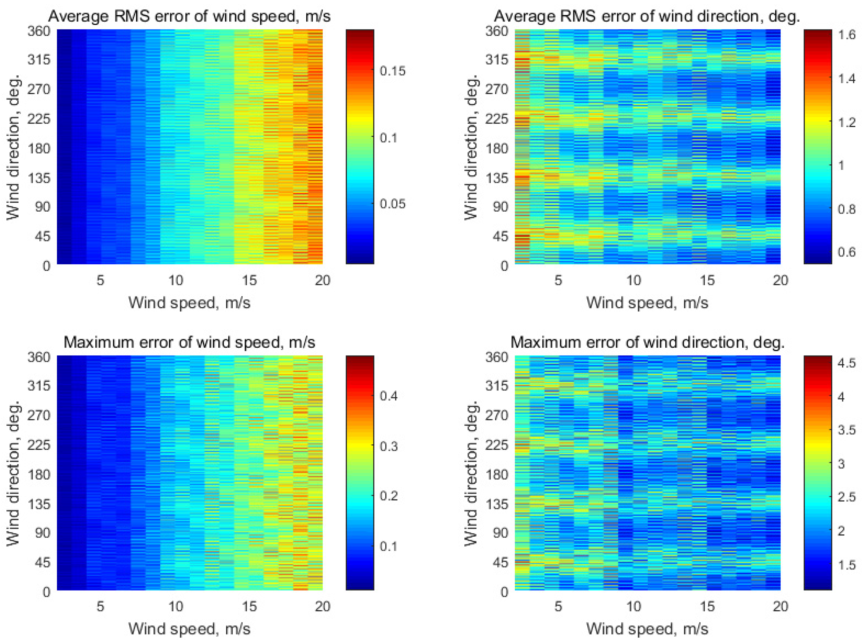
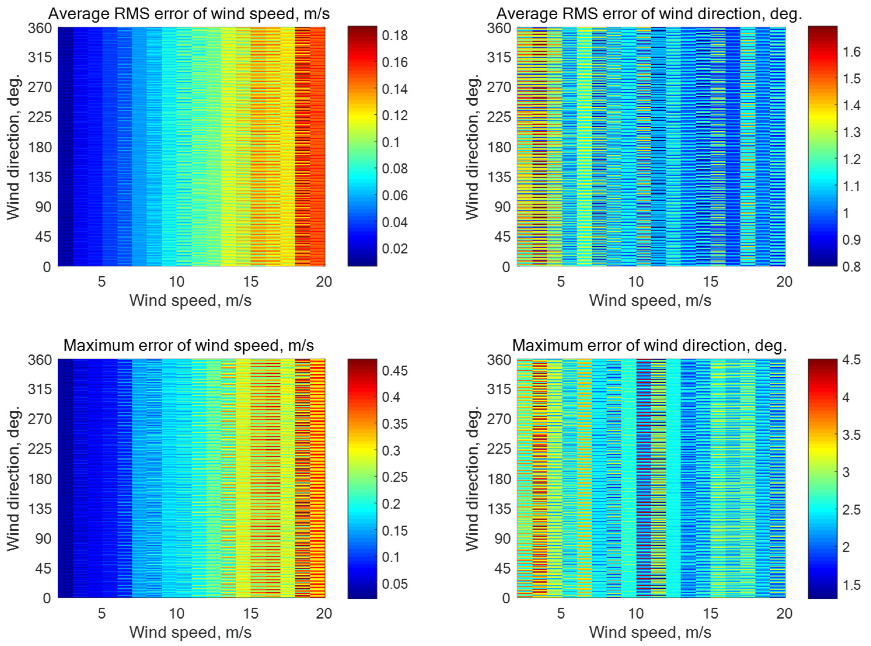
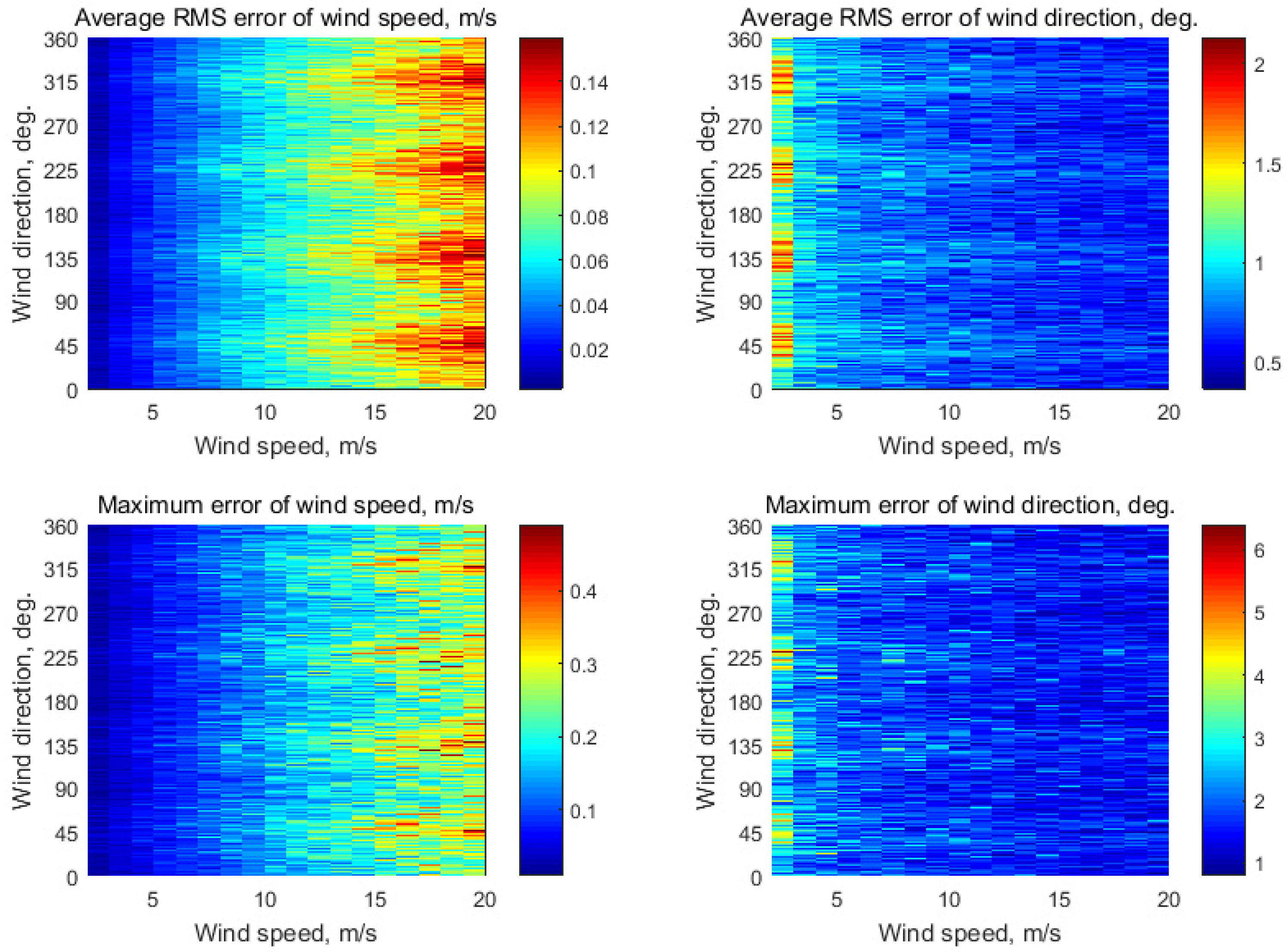
The simulations have been done assuming a 0.2 dB instrumental noise. This value of the instrumental noise had been reported for the ERS-1 scatterometer, and we considered this value as a worse case, readily achievable for airborne scatterometers. The results for the narrow, medium, and wide cases at the incidence angle of 45° are presented in Figure 2, Figure 3 and Figure 4, respectively. In the narrow case, the maximum errors of retrieval of the wind speed and direction are 0.49 m/s and 5.1° (Figure 2). At the medium width, the maximum errors are a little bit higher and are 0.52 m/s and 5.7° (Figure 3). And, when the nose, tail, and wings are wide, the maximum errors are almost the same values of 0.54 m/s and 5.6° (Figure 4). The average RMS error of the wind speed and direction also for the cases considered are presented in appropriate figures. As expected, they have low values: about 0.2 m/s and 1.8° in the narrow case (Figure 2), 0.18 m/s and 1.9° in the medium case (Figure 3), and 0.19 m/s and 2° in the wide case (Figure 4) that also indicate the quality of the wind retrieval.
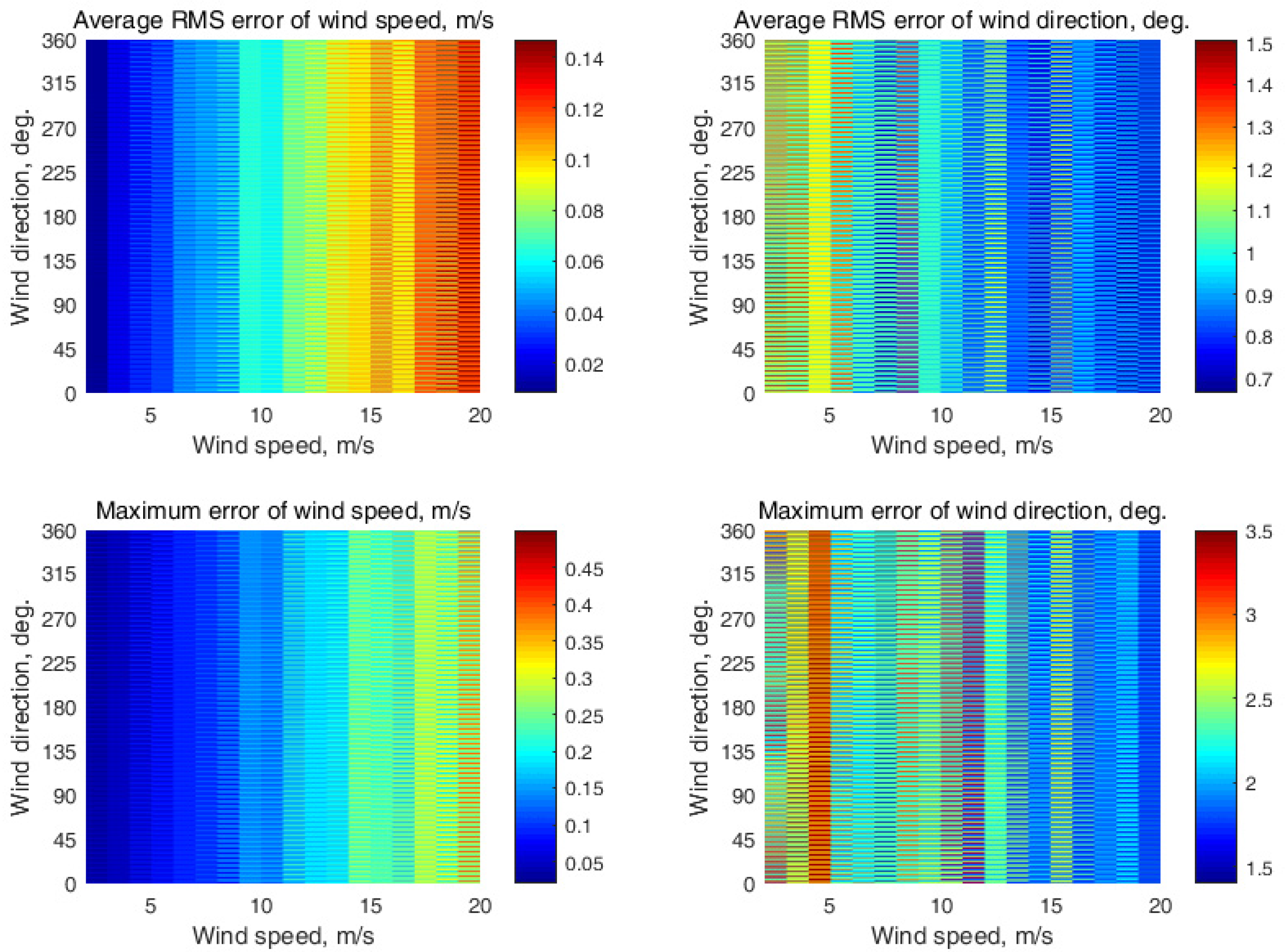
At the same time, the results for the narrow, medium, and wide cases at the incidence angle of 60° are shown in Figure 5, Figure 6 and Figure 7, respectively. In the narrow case, the maximum errors of retrieval of the wind speed and direction are 0.49 m/s and 4.6° (Figure 5). At the medium width, the maximum errors are a little bit higher and are 0.5 m/s and 5.0° (Figure 6). And, when the nose, tail, and wings are wide, the maximum errors are almost the same values of 0.49 m/s and 5.4° (Figure 7). The average RMS error of the wind speed and direction also for the cases considered are presented in appropriate figures. They also have low values: about 0.18 m/s and 1.6° in the narrow case (Figure 5), 0.17 m/s and 1.7° in the medium case (Figure 6), and 0.16 m/s and 1.7° in the wide case (Figure 7) that also demonstrate the quality of the wind retrieval.
These results clearly show the suitability of the airborne rotating-beam scatterometer mounted over the fuselage for the sea wind measurement. Although the NRCSs of the underlying water surface are not available from the azimuth sectors shadowed by the nose, tail, and wings, all three cases considered have demonstrated very good simulation results. Despite that wider nose, tail, and wings lead to some increase of the wind speed and direction measurement errors, these errors are within the typical accuracy ranges of ±2 m/s and ±20° of the scatterometer wind measurement [34]. E.g., the following wind speed and direction accuracy of modern scatterometers have been specified as: 2 m/s at wind speeds 4–20 m/s (or 10% if larger) and 20 for CFOSAT SCAT [35]; 2 m/s at wind speeds 3–20 m/s and 20 for ISS RapidScat [36].
The higher wind speed leads to an increase of the wind speed measurement error and, at the same time, leads to a decrease of the wind direction measurement error. It is due to the features of the microwave backscattering from water at medium incidence angles. The water NRCS increases with the wind speed increase but NRCS increases slower at higher wind speed than at lower one. And so, the higher wind speed leads to the higher error of the wind speed measurement. At the same time, an increase of the wind speed changes the anisotropic properties of the water backscatter increasing the difference between the maxima and minima of the NRCS azimuth curve and between the main and the second maxima (at the same incidence angle) that leads to decrease of the wind direction measurement error.
Besides that, it was very interesting to compare the potential of these three cases with the case when the measurement of the whole 360° azimuthal NRCS curve of the water surface is available (e.g., with the airborne scatterometer having the rotating-beam antenna mounted at the bottom or under the fuselage), and with the case when only four azimuth sectors at the directions of 45°, 135°, 225°, and 315° are evadible for the NRCS measurement (e.g., in the case of the airborne Doppler navigation system geometry [37,38]).
At this comparison, we also have used our previous result corresponding to the case of N = 72 azimuth sectors (No shadows case in Table 1) at the directions of 0°, 5°, 10°, …, 355° from [30] presented here in Appendix A, and a new result corresponding to the case of N = 4 azimuth sectors at the directions of 45°, 135°, 225°, and 315° presented here in Appendix B.
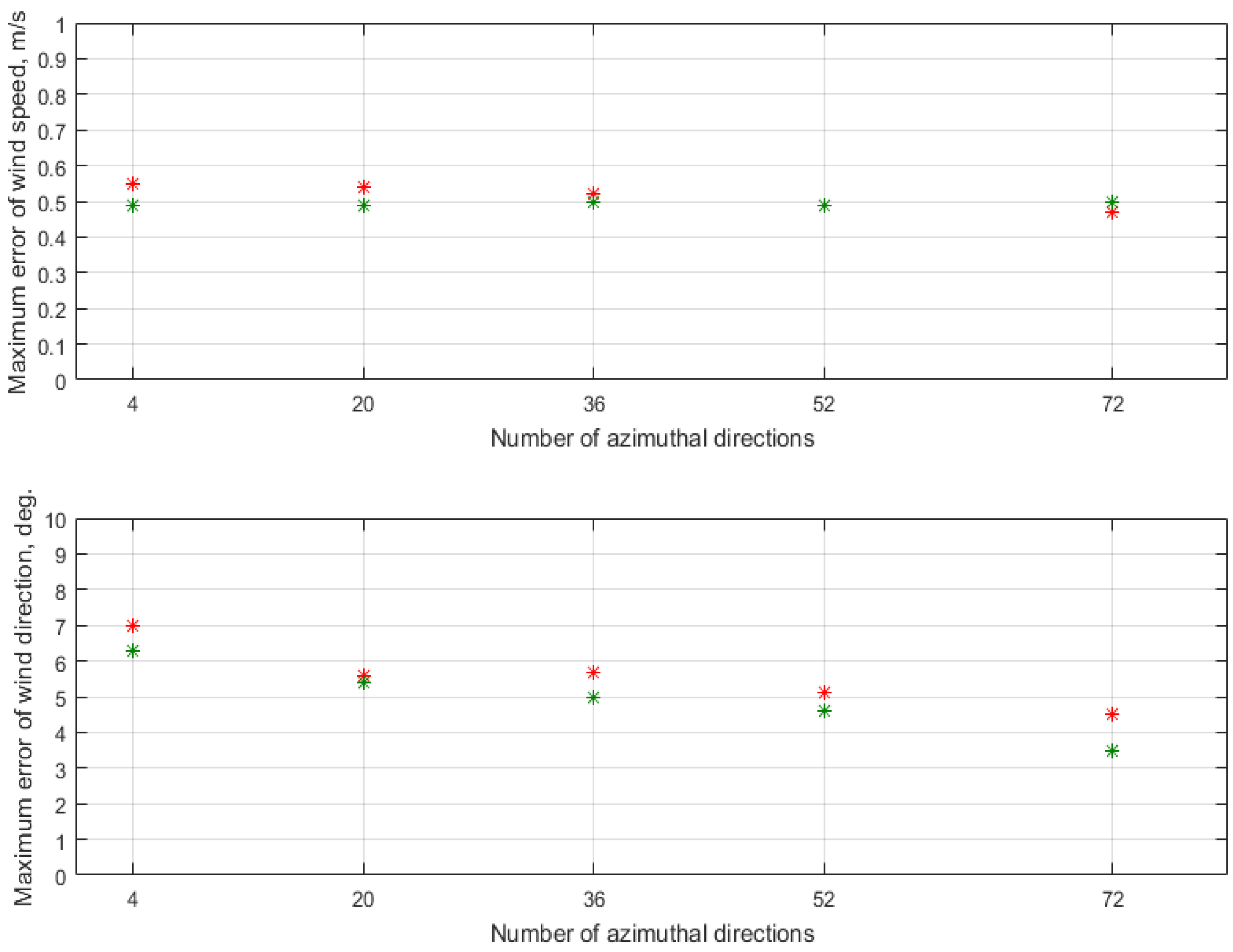
The comparative results have been shown in Figure 8. This comparison has shown that the lowest errors of the wind speed and direction are achieved when the whole 360° azimuthal NRCS curve of the water surface is available, and the highest errors of the wind speed and wind direction recovery take place when only four NRCS measurements are evadible from the azimuth directions of 45°, 135°, 225°, and 315°. In the cases of the narrow, medium, and wide nose, tail, and wings, the errors of the wind speed and direction recovery have intermediate values. The wind retrieval errors increase slightly when the number of the observed azimuth sectors decreases. The errors at the incidence angle of 45° are only slightly higher than at the incidence angle of 60°. In any case, the errors of the wind speed and direction recovery in all the cases are within their typical values of the scatterometer measurement. And so, an airborne rotating-beam scatterometer mounted over the fuselage is feasible well for the sea wind measurement allowing the wind speed and direction retrieval with a little higher errors than it is possible in the best case of the airborne scatterometer with the rotating-beam antenna mounted at the bottom or under the fuselage when the whole 360° azimuthal NRCS curve of the water surface is available at the measurement.
Also, these results demonstrate that functionality of the airborne rotating-beam radars mounted over the fuselage (e.g., AEW systems [21,39]) can be enhanced to provide the sea wind measurement in addition to their typical applications. For that reason, the airborne rotating-beam radar should operate in the scatterometer mode and conduct the NRCS measurement of the underlying water surface at medium incidence angles.
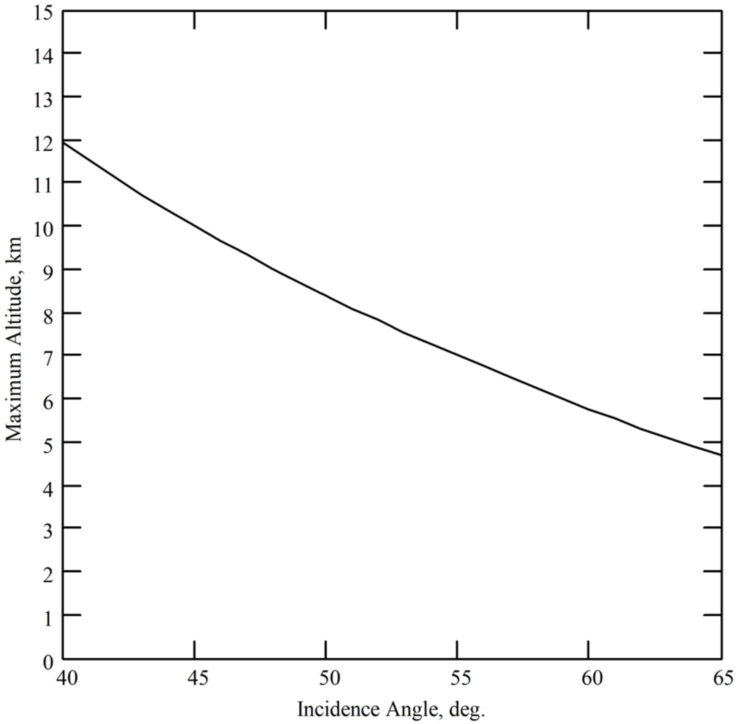
The altitude limitation for the wind retrieval by the airborne scatterometer with the rotating-beam antenna is determined by the area observed in which the observation circle traced at the same incidence angle on the water surface is included, and the assumed wind and wave conditions are identical (can be considered to be the same at all the part of the area, like it is assumed for the satellite scatterometer selected cell). Typically, the dimensions of such an area are about 15–20 km, and so the wind measurement maximum altitude is about 10 km at the incidence angle of 45°. Thus, e.g., if the airborne radar with the rotating-beam antenna provides the observations at the incidence angle of 60° (e.g., in the case of the AEW systems), the maximum altitude of the wind measurement in the scatterometer mode can be only about 5.77 km (Figure 9).
The higher maximum altitude of the method’s applicability always is preferable as it provides a larger range of acceptable flight altitudes allowing flexibility in flight plans. Also, we have taken into account that the 45° incidence angle is within the incidence angles commonly used by other airborne scatterometers. So, one reason to use the incidence angle of 45° is to increase the maximum altitude to about 10 km in comparison with the maximum altitude of 5.77 km achievable at the incidence angle of 60°. Another reason to use the incidence angle of 45° is that the anisotropic properties of the water backscatter (the difference between the maxima and minima of the NRCS azimuth curve and between the main and the second maxima at the same incidence angle) are stronger at higher incidence angles then at the incidence angle of 30° that provides more precise retrieval of the wind direction [40]. Recently, we have demonstrated in [30] the superiority of the scatterometer wind recovery at the incidence angles higher than 30°, as a significantly higher number of integrated NRCSs are required at the 30° incidence angle to achieve similar wind retrieval accuracy.
Therefore, to increase the maximum altitude of the method’s applicability and ensure the accuracy of the wind recovery, the incidence angle of measurements should at least tend to 45° when enhancing the functionality of the airborne radar with the rotating-beam antenna mounted over the fuselage to measure the wind over the sea in the scatterometer mode.
The spatial variability or other wind and water features not taken into account by the GMF also may affect the wind vector recovery. To reduce their influence on the wind measurement, several circular scans are applied by the airborne scatterometer to increase the number of integrated NRCS samples for each azimuth sector [8].
4. Conclusions
The analysis of the airborne radar with the rotating-beam antenna mounted over the fuselage and operated in the scatterometer mode has shown that it is feasible for the sea wind measurement in all three considered cases of narrow, medium, and wide nose, tail, and wings.
Despite the fact that the NRCSs of the underlying water surface are not available from some azimuth sectors due to their shadowing by the nose, tail, and wings, the errors of the wind speed and direction recovery are only slightly higher than in the no-shadow case when the measurement of the whole 360° azimuthal NRCS curve of the water surface is available, e.g., when the airborne scatterometer with the rotating-beam antenna is mounted at the bottom or under the fuselage, but still within the ranges of the typical accuracy of ±2 m/s and ±20° of the scatterometer wind measurement. Thus, an airborne rotating-beam scatterometer mounted over the fuselage is feasible well for the sea wind measurement, especially when the scatterometer could not be mounted under the fuselage by specificity of aircraft, or existent airborne radar mounted over the fuselage is enhanced its functionality.
The functionality of the airborne rotating-beam radars installed over the fuselage can also be enhanced to provide the sea wind recovery in addition to their typical applications. For that purpose, the airborne rotating-beam radar should operate in the scatterometer mode and provide the NRCS measurement of the underlying water surface at medium incidence angle. To ensure the accuracy of the wind recovery increasing the maximum altitude of the method’s applicability, the incidence angle at the measurements should be about 45°, or at least tend to 45°.
Thus, the obtained results can be essential in the development of new remote sensing systems or functionality enhancement of the existent airborne radars providing their use for the sea wind measurement.
Author Contributions
Conceptualization, A.N.; methodology, A.N. and A.K.; software, A.K.; validation, A.N. and A.K.; formal analysis, A.N. and A.K.; investigation, A.N. and A.K.; resources, A.K.; data curation, A.N. and A.K.; writing—original draft preparation, A.N.; writing—review & editing, A.N. and A.K.; visualization, A.N. and A.K.; supervision, A.N.; project administration, A.K.; funding acquisition, A.K. All authors have read and agreed to the published version of the manuscript.
Funding
This research was funded by the Russian Science Foundation grant number 21-79-10375, https://rscf.ru/en/project/21-79-10375/ (accessed on 6 November 2021). The APC was funded by the Russian Science Foundation grant number 21-79-10375.
Data Availability Statement
Data sharing not applicable.
Conflicts of Interest
The authors declare no conflict of interest.
Appendix A
The simulation results of the wind retrieval by Equation (2) in the case of the seventy-two-beam star geometry (N = 72) from [30] are presented here. The whole 360° azimuthal NRCS curve is available in that case that is equivalent to the case of the observation N = 72 azimuth sectors at the directions of 0°, 5°, 10°, …, 355° relative to the aircraft course when the nose, tail, and wings do not shadow any part of the water surface. It takes place when an airborne scatterometer with the rotating-beam antenna is mounted at the bottom or under the fuselage. This simulation have been performed using Monte Carlo simulations, a Rayleigh Power (Exponential) distribution, and a GMF of the form of Equation (1) with the coefficients for transmitting and receiving at the horizontal polarization (Equation (5)). The simulation results with an assumption of 0.2 dB instrumental noise at the wind speeds of 2–20 m/s for the incidence angles of 45° and 60° with 87 integrated NRCS samples for each azimuth sector are presented in Figure A1 and Figure A2, respectively.
Figure A1.
Simulation results in the case of the observation N = 72 azimuth sectors at the directions of 0°, 5°, 10°, …, 355° relative to the aircraft course with an assumption of 0.2 dB instrumental noise at the wind speeds of 2–20 m/s for the incidence angle of 45° with 87 integrated NRCS samples for each azimuth sector.

The maximum errors of the wind speed and direction recovery are 0.47 m/s and 4.5°, and 0.5 m/s and 3.5°, respectively, at the incidence angles of 45° and 60°. Thus, the errors are within the ranges of the typical accuracy of ±2 m/s and ±20° of the scatterometer wind measurement [34].
Figure A2.
Simulation results in the case of the observation N = 72 azimuth sectors at the directions of 0°, 5°, 10°, …, 355° relative to the aircraft course with an assumption of 0.2 dB instrumental noise at the wind speeds of 2–20 m/s for the incidence angle of 60° with 87 integrated NRCS samples for each azimuth sector.

Appendix B
To compare the wind retrieval potential in the cases of narrow, medium, and wide nose, tail, and wings, we also needed to simulate the wind retrieval in the contrary case when only N = 4 azimuth sectors at the directions of 45°, 135°, 225°, and 315° relative to the aircraft course are evadible.
In that case, the following system of four equations has been used for the wind retrieval:
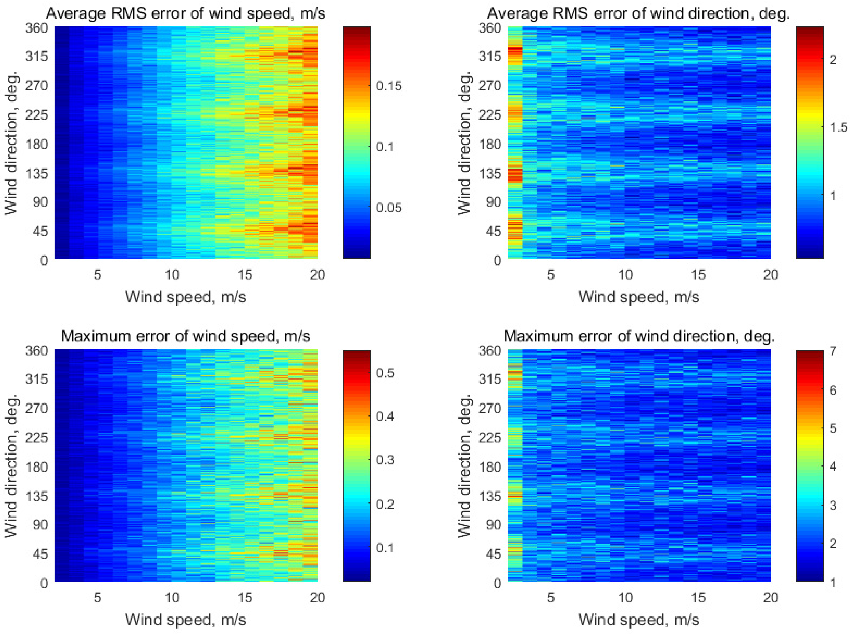
As before, the results have been obtained using Monte Carlo simulations, a Rayleigh Power (Exponential) distribution, and a GMF of the form of Equation (1) with the coefficients for transmitting and receiving at the horizontal polarization (Equation (5)) with an assumption of 0.2 dB instrumental noise at the wind speeds of 2–20 m/s for the incidence angles of 45° and 60° with 1565 integrated NRCS samples for each azimuth sector. These simulation results are shown in Figure A3 and Figure A4, respectively.
Figure A3.
Simulation results in the case of the observation N = 4 azimuth sectors at the directions of 45°, 135°, 225°, and 315° relative to the aircraft course with an assumption of 0.2 dB instrumental noise at the wind speeds of 2–20 m/s for the incidence angle of 45° with 1565 integrated NRCS samples for each azimuth sector.

Figure A4.
Simulation results in the case of the observation N = 4 azimuth sectors at the directions of 45°, 135°, 225°, and 315° relative to the aircraft course with an assumption of 0.2 dB instrumental noise at the wind speeds of 2–20 m/s for the incidence angle of 60° with 1565 integrated NRCS samples for each azimuth sector.

The maximum errors of the wind speed and direction recovery are 0.55 m/s and 7° and 4.5°, and 0.49 m/s and 6.3°, respectively, at the incidence angles of 45° and 60°. As we can see, the errors in this contrary case (to the case of Appendix A) are also within the ranges of the typical accuracy of ±2 m/s and ±20° of the scatterometer wind measurement [34].
References
- Njoku, E.G. Encyclopedia of Remote Sensing; Springer: New York, NY, USA, 2014; p. 939. ISBN 978-0-387-36700-2. [Google Scholar]
- Active Earth Remote Sensing for Ocean Applications. In A Strategy for Active Remote Sensing Amid Increased Demand for Radio Spectrum; The National Academies Press: Washington, DC, USA, 2015; pp. 54–76. ISBN 0-309-37305-0. Available online: https://www.nap.edu/read/21729/chapter/5 (accessed on 6 November 2021).
- Oberthaler, K.; Thompson, A. Wind and the Wires: A History of Scatterometry. 2010. Available online: https://cresis.ku.edu/content/news/newsletter/927 (accessed on 6 November 2021).
- Liu, W.T. Progress in scatterometer application. J. Oceanogr. 2002, 58, 121–136. [Google Scholar] [CrossRef]
- Giovanangeli, J.-P.; Bliven, L.F.; Calve, O.L. A Wind-wave tank study of the azimuthal response of a Ka-band scatterometer. IEEE Trans. Geosci. Remote Sens. 1991, 29, 143–148. [Google Scholar] [CrossRef]
- Snoeijl, P.; Van Halsema, D.; Oost, W.A.; Calkoen, C.; Jaehne, B.; Vogelzang, J. Microwave backscatter measurements made from the Dutch ocean research tower ‘Noordwijk’ compared with model predictions. In Proceedings of the IGARSS’92, Houston, TX, USA, 26–29 May 1992; pp. 696–698. [Google Scholar] [CrossRef]
- Wismann, V. Ocean windfield measurements with a rotating antenna airborne C-band scatterometer. In Proceedings of the 12th Canadian Symposium on Remote Sensing Geoscience and Remote Sensing Symposium, Vancouver, BC, Canada, 10–14 July 1989; pp. 1470–1473. [Google Scholar] [CrossRef]
- Carswell, J.R.; Carson, S.C.; McIntosh, R.E.; Li, F.K.; Neumann, G.; McLaughlin, D.J.; Wilkerson, J.C.; Black, P.G.; Nghiem, S.V. Airborne scatterometers: Investigating ocean backscatter under low-and high-wind conditions. Proc. IEEE 1994, 82, 1835–1860. [Google Scholar] [CrossRef]
- Jones, W.L. Early days of microwave scatterometry: RADSCAT to SASS. In Proceedings of the 2015 IEEE International Geoscience and Remote Sensing Symposium, Milan, Italy, 26–31 July 2015; pp. 4208–4211. [Google Scholar] [CrossRef]
- Xu, X.; Dong, X.; Xie, Y. On-Board Wind Scatterometry. Remote Sens. 2020, 12, 1216. [Google Scholar] [CrossRef] [Green Version]
- Karaev, V.Y.; Panfilova, M.A.; Titchenko, Y.A.; Meshkov, E.M.; Balandina, G.N.; Kuznetsov, Y.V.; Shlaferov, A.L. Retrieval of the near-surface wind velocity and direction: SCAT-3 orbit-borne scatterometer. Radiophys. Quantum Electron. 2016, 59, 259–269. [Google Scholar] [CrossRef]
- Spencer, M.W.; Graf, J.E. The NASA scatterometer (NSCAT) mission. Backscatter 1997, 8, 18–24. [Google Scholar]
- Moore, R.K. Radar sensing of the ocean. IEEE J. Ocean. Eng. 1985, 10, 84–113. [Google Scholar] [CrossRef]
- Moore, R.K.; Fung, A.K. Radar determination of winds at sea. Proc. IEEE 1979, 67, 1504–1521. [Google Scholar] [CrossRef]
- Masuko, H.; Okamoto, K.; Shimada, M.; Niwa, S. Measurement of microwave backscattering signatures of the ocean surface using X band and Ka band airborne scatterometers. J. Geophys. Res. Oceans 1986, 91, 13065–13083. [Google Scholar] [CrossRef]
- Fernandez, D.E.; Kerr, E.; Castells, A.; Frasier, S.; Carswell, J.; Chang, P.S.; Black, P.; Marks, F. IWRAP: The Imaging Wind and Rain Airborne Profiler for remote sensing of the ocean and the atmospheric boundary layer within tropical cyclones. IEEE Trans. Geosci. Remote Sens. 2005, 43, 1775–1787. [Google Scholar] [CrossRef]
- Jones, W.L.; Schroeder, L.C.; Mitchell, J.L. Aircraft measurements of the microwave scattering signature of the ocean. IEEE Trans. Antennas Propag. 1977, AP-25, 52–61. [Google Scholar] [CrossRef]
- Unal, C.M.H.; Snoeij, P.; Swart, P.J.F. The polarization-dependent relation between radar backscatter from the ocean surface and surface wind vectors at frequencies between 1 and 18 GHz. IEEE Trans. Geosci. Remote Sens. 1991, 29, 621–626. [Google Scholar] [CrossRef]
- Rodríguez, E.; Wineteer, A.; Perkovic-Martin, D.; Gál, T.; Stiles, B.W.; Niamsuwan, N.; Rodriguez Monje, R. Estimating ocean vector winds and currents using a Ka-band pencil-beam Doppler scatterometer. Remote Sens. 2018, 10, 576. [Google Scholar] [CrossRef] [Green Version]
- Li, Z.; Stoffelen, A.; Verhoef, A. A generalized simulation capability for rotating-beam scatterometers. Atmos. Meas. Tech. 2019, 12, 3573–3594. [Google Scholar] [CrossRef] [Green Version]
- Kramer, H.J. Observation of the Earth and Its Environment: Survey of Missions and Sensors, 4th ed.; Springer: Berlin/Heidelberg, Germany, 2002; p. 1509. [Google Scholar] [CrossRef] [Green Version]
- Hildebrand, P.H. Estimation of sea-surface wind using backscatter cross-section measurements from airborne research weather radar. IEEE Trans. Geosci. Remote Sens. 1994, 32, 110–117. [Google Scholar] [CrossRef]
- Nekrasov, A.; Dell’Acqua, F. Airborne Weather Radar: A theoretical approach for water-surface backscattering and wind measurements. IEEE Geosci. Remote Sens. Mag. 2016, 4, 38–50. [Google Scholar] [CrossRef]
- Nekrasov, A.; Khachaturian, A.; Veremyev, V.; Bogachev, M. Sea surface wind measurement by airborne weather radar scanning in a wide-size sector. Atmosphere 2016, 7, 72. [Google Scholar] [CrossRef] [Green Version]
- Nekrasov, A.; De Wit, J.J.M.; Hoogeboom, P. FM-CW millimeter wave demonstrator system as a sensor of the sea surface wind vector. IEICE Electron. 2004, 1, 137–143. [Google Scholar] [CrossRef] [Green Version]
- Nekrasov, A. Airborne Doppler navigation system application for measurement of the water surface backscattering signature. In Proceedings of the ISPRS TC VII Symposium—100 Years ISPRS, Vienna, Austria, 5–7 July 2010; Wagner, W., Székely, B., Eds.; The International Archives of the Photogrammetry, Remote Sensing and Spatial Information Sciences. 2010; Volume XXXVIII, pp. 163–168. Available online: https://www.isprs.org/proceedings/XXXVIII/part7/a/pdf/163_XXXVIII-part7A.pdf (accessed on 6 November 2021).
- Nekrasov, A.; Veremyev, V. Airborne weather radar concept for measuring water surface backscattering signature and sea wind at circular flight. Nase More 2016, 63, 278–282. [Google Scholar] [CrossRef]
- Nekrasov, A.; Popov, D. A concept for measuring the water-surface backscattering signature by airborne weather radar. In Proceedings of the 16th International Radar Symposium IRS 2015, Dresden, Germany, 24–26 June 2015; Volume 2, pp. 1112–1116. [Google Scholar] [CrossRef]
- Nekrasov, A.; Khachaturian, A.; Veremyev, V.; Bogachev, M. Doppler navigation system with a non-stabilized antenna as a sea-surface wind sensor. Sensors 2017, 17, 1340. [Google Scholar] [CrossRef] [Green Version]
- Nekrasov, A.; Khachaturian, A.; Abramov, E.; Popov, D.; Markelov, O.; Obukhovets, V.; Veremyev, V.; Bogachev, M. Optimization of airborne antenna geometry for ocean surface scatterometric measurements. Remote Sens. 2018, 10, 1501. [Google Scholar] [CrossRef] [Green Version]
- Nekrassov, A. Sea surface wind vector measurement by airborne scatterometer having wide-beam antenna in horizontal plane. In Proceedings of the IGARSS’99, Hamburg, Germany, 28 June–2 July 1999; Volume 2, pp. 1001–1003. [Google Scholar] [CrossRef]
- Nekrassov, A. On airborne measurement of the sea surface wind vector by a scatterometer (altimeter) with a nadir-looking wide-beam antenna. IEEE Trans. Geosci. Remote Sens. 2002, 40, 2111–2116. [Google Scholar] [CrossRef]
- Hans, P. Auslegung und Analyse von Satellitengetragenen Mikrowellensensorsystemen zur Windfeldmessung (Scatterometer) Über Dem Meer und Vergleich der Meßverfahren in Zeit- und Frequenzebene. Von der Fakultät 2 Bauingenieur- und Vermessungswesen der Universität Stuttgart zur Erlangung der Würde eines Doktor-Ingenieurs Genehmigte Abhandlung; Institut für Navigation der Universität Stuttgart: Stuttgart, Germany, 1987; p. 225S. (In German) [Google Scholar]
- Komen, G.J.; Cavaleri, L.; Donelan, M.; Hasselmann, K.; Hasselmann, S.; Janssen, P.A.E.M. Dynamics and Modelling of Ocean Waves; Cambridge University Press: Cambridge, UK, 1994; p. 532. [Google Scholar]
- CFOSAT. Available online: https://directory.eoportal.org/web/eoportal/satellite-missions/c-missions/cfosat (accessed on 6 November 2021).
- RapidScat Instrument Overview. Available online: https://spaceflight101.com/iss/rapidscat/ (accessed on 6 November 2021).
- Nekrasov, A. Measuring the sea surface wind vector by the Doppler navigation system of flying apparatus having the track-stabilized four-beam antenna. In Proceedings of the 17th Asia Pacific Microwave Conference (APMC), Suzhou, China, 4–7 December 2005; Volume 1, pp. 645–647. [Google Scholar] [CrossRef]
- Nekrasov, A.; Khachaturian, A.; Veremyev, V.; Bogachev, M. Sea wind measurement by Doppler navigation system with x-configured beams at rectilinear fight. Remote Sens. 2017, 17, 887. [Google Scholar] [CrossRef] [Green Version]
- Long, M.W. Airborne Early Warning System Concepts; SciTech Publishing Inc.: Raleigh, NC, USA, 2004; p. 476. ISBN 978-1-891121-32-6. [Google Scholar]
- Ulaby, F.T.; Moore, R.K.; Fung, A.K. Microwave Remote Sensing: Active and Passive, Volume II: Radar Remote Sensing and Surface Scattering and Emission Theory; Addison-Wesley: London, UK, 1982; p. 1064. [Google Scholar]
Figure 1.
Azimuth sectors available for the underlying surface NRCS observation at the medium incidence angles and sectors shadowed by the aircraft’s nose, tail, and wings when the rotating-beam radar is mounted over the fuselage.
Figure 1.
Azimuth sectors available for the underlying surface NRCS observation at the medium incidence angles and sectors shadowed by the aircraft’s nose, tail, and wings when the rotating-beam radar is mounted over the fuselage.

Figure 2.
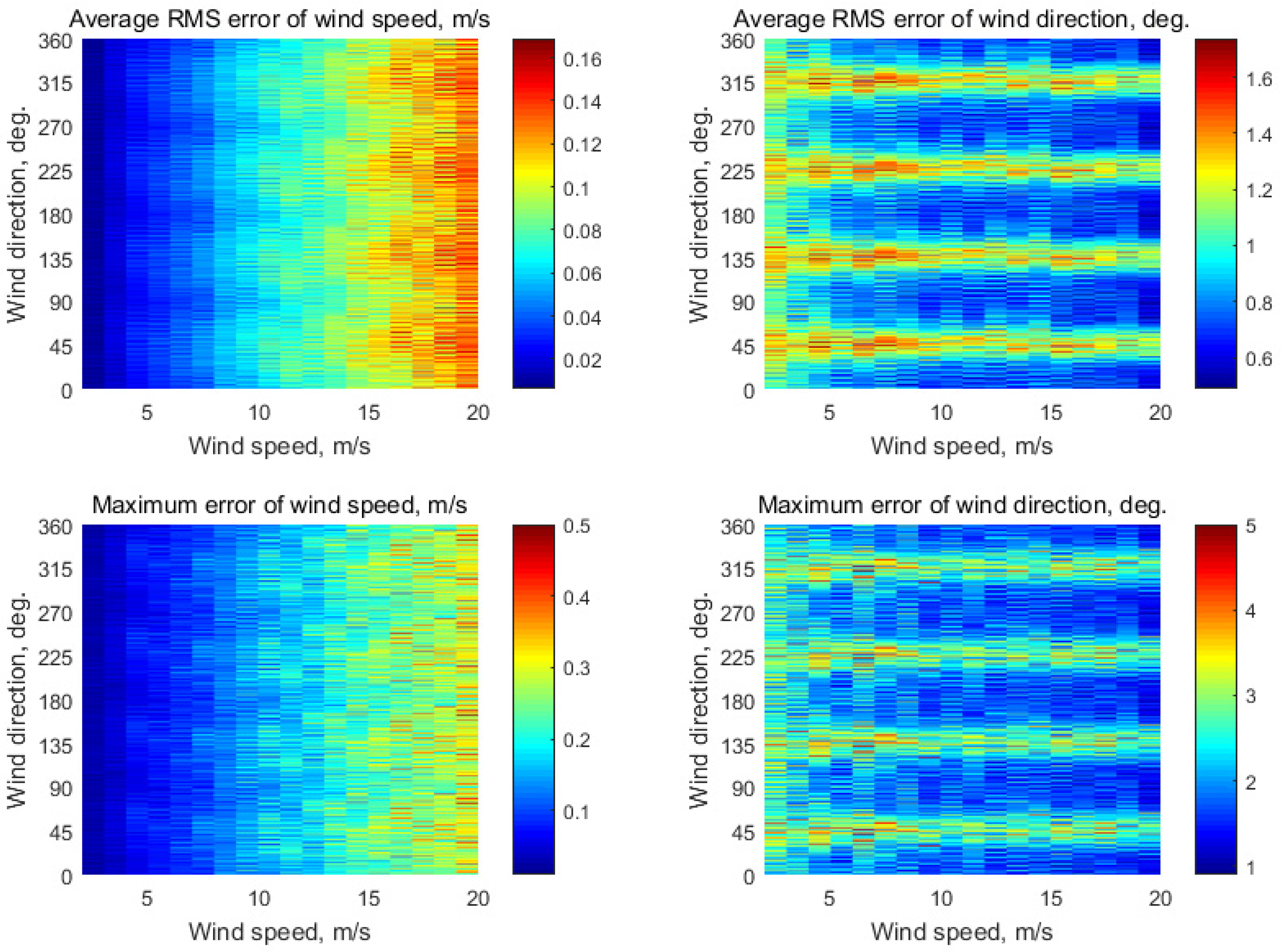
Simulation results in the case of the narrow nose, tail, and wings (N = 52) with an assumption of 0.2 dB instrumental noise at the wind speeds of 2–20 m/s for the incidence angle of 45° with 120 integrated NRCS samples for each azimuth sector.
Figure 2.
Simulation results in the case of the narrow nose, tail, and wings (N = 52) with an assumption of 0.2 dB instrumental noise at the wind speeds of 2–20 m/s for the incidence angle of 45° with 120 integrated NRCS samples for each azimuth sector.

Figure 3.
Simulation results in the case of the medium nose, tail, and wings (N = 36) with an assumption of 0.2 dB instrumental noise at the wind speeds of 2–20 m/s for the incidence angle of 45° with 174 integrated NRCS samples for each azimuth sector.
Figure 3.
Simulation results in the case of the medium nose, tail, and wings (N = 36) with an assumption of 0.2 dB instrumental noise at the wind speeds of 2–20 m/s for the incidence angle of 45° with 174 integrated NRCS samples for each azimuth sector.

Figure 4.
Simulation results in the case of the wide nose, tail, and wings (N = 20) with an assumption of 0.2 dB instrumental noise at the wind speeds of 2–20 m/s for the incidence angle of 45° with 313 integrated NRCS samples for each azimuth sector.
Figure 4.
Simulation results in the case of the wide nose, tail, and wings (N = 20) with an assumption of 0.2 dB instrumental noise at the wind speeds of 2–20 m/s for the incidence angle of 45° with 313 integrated NRCS samples for each azimuth sector.

Figure 5.
Simulation results in the case of the narrow nose, tail, and wings (N = 52) with an assumption of 0.2 dB instrumental noise at the wind speeds of 2–20 m/s for the incidence angle of 60° with 120 integrated NRCS samples for each azimuth sector.
Figure 5.
Simulation results in the case of the narrow nose, tail, and wings (N = 52) with an assumption of 0.2 dB instrumental noise at the wind speeds of 2–20 m/s for the incidence angle of 60° with 120 integrated NRCS samples for each azimuth sector.

Figure 6.
Simulation results in the case of the medium nose, tail, and wings (N = 36) with an assumption of 0.2 dB instrumental noise at the wind speeds of 2–20 m/s for the incidence angle of 60° with 174 integrated NRCS samples for each azimuth sector.
Figure 6.
Simulation results in the case of the medium nose, tail, and wings (N = 36) with an assumption of 0.2 dB instrumental noise at the wind speeds of 2–20 m/s for the incidence angle of 60° with 174 integrated NRCS samples for each azimuth sector.

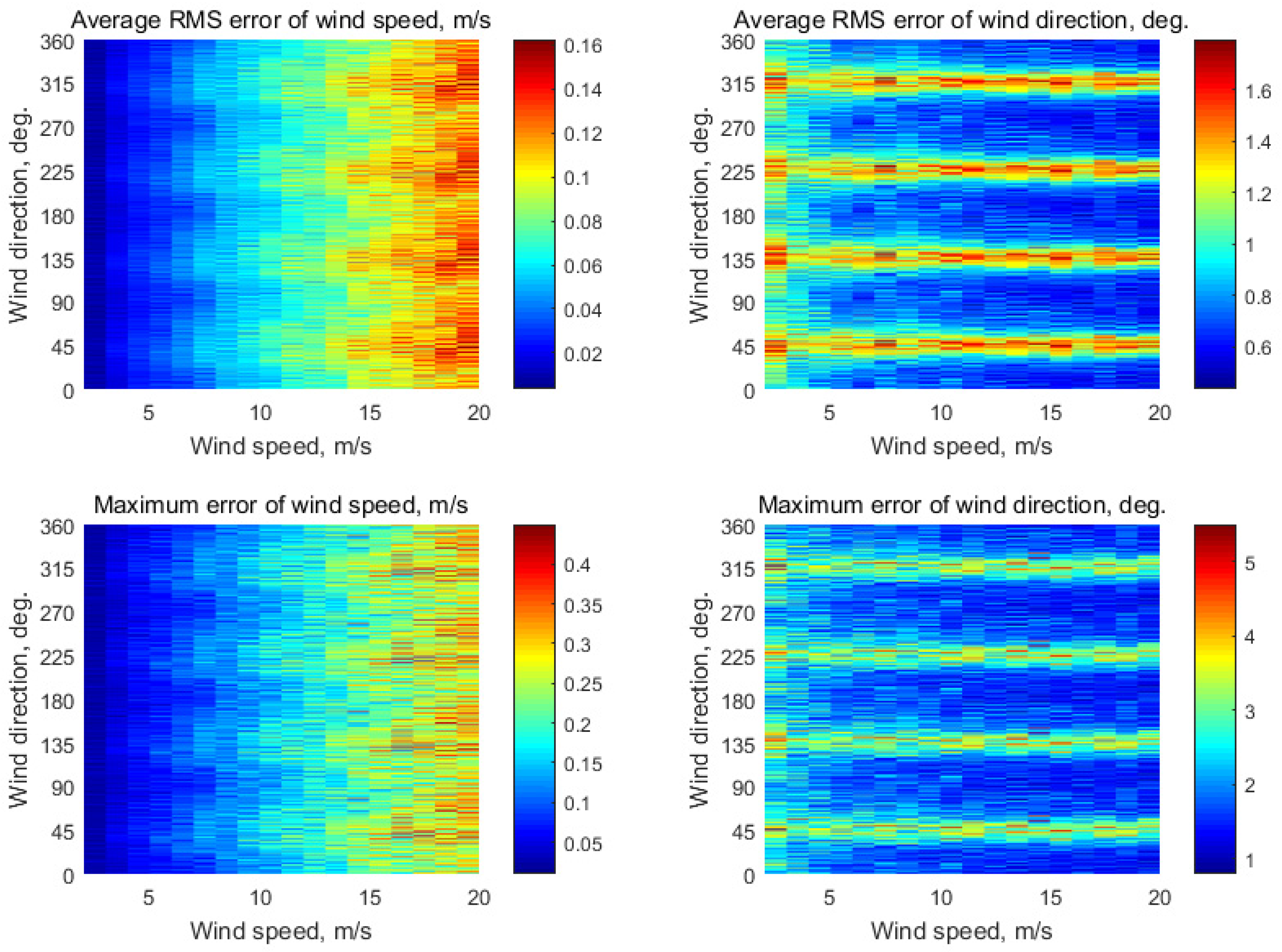
Figure 7.
Simulation results in the case of the wide nose, tail, and wings (N = 20) with an assumption of 0.2 dB instrumental noise at the wind speeds of 2–20 m/s for the incidence angle of 60° with 313 integrated NRCS samples for each azimuth sector.
Figure 7.
Simulation results in the case of the wide nose, tail, and wings (N = 20) with an assumption of 0.2 dB instrumental noise at the wind speeds of 2–20 m/s for the incidence angle of 60° with 313 integrated NRCS samples for each azimuth sector.

Figure 8.
Comparative results of the maximum wind retrieval errors in the case of the whole 360° azimuthal NRCS curve available (N = 72), in the cases of the narrow, medium, and wide nose, tail, and wings (N = 52, 36, and 20, respectively), and in the case when only four azimuth sectors at the directions of 45°, 135°, 225°, and 315° are evadible: red asterisks are for the incidence angle of 45°, and green asterisks are for the incidence angle of 60°.

Figure 9.
The maximum altitude dependence on the incidence angle.


Table 1.
Sectors shadowed and observed in different cases of observation.
| Azimuth of Sector | No Shadows Case N = 72 | Narrow Shadows Case N = 52 | Medium Shadows Case N = 36 | Wide Shadows Case N = 20 | ||||
|---|---|---|---|---|---|---|---|---|
| Sector Status | Number of Observed Sector i | Sector Status | Number of Observed Sector i | Sector Status | Number of Observed Sector i | Sector Status | Number of Observed Sector i | |
| 0° | observed | 1 | shadowed by the nose | – | shadowed by the nose | – | shadowed by the nose | – |
| 5° | observed | 2 | shadowed by the nose | – | shadowed by the nose | – | shadowed by the nose | – |
| 10° | observed | 3 | shadowed by the nose | – | shadowed by the nose | – | shadowed by the nose | – |
| 15° | observed | 4 | observed | 1 | shadowed by the nose | – | shadowed by the nose | – |
| 20° | observed | 5 | observed | 2 | shadowed by the nose | – | shadowed by the nose | – |
| 25° | observed | 6 | observed | 3 | observed | 1 | shadowed by the nose | – |
| 30° | observed | 7 | observed | 4 | observed | 2 | shadowed by the nose | – |
| 35° | observed | 8 | observed | 5 | observed | 3 | observed | 1 |
| 40° | observed | 9 | observed | 6 | observed | 4 | observed | 2 |
| 45° | observed | 10 | observed | 7 | observed | 5 | observed | 3 |
| 50° | observed | 11 | observed | 8 | observed | 6 | observed | 4 |
| 55° | observed | 12 | observed | 9 | observed | 7 | observed | 5 |
| 60° | observed | 13 | observed | 10 | observed | 8 | shadowed by the right wing | – |
| 65° | observed | 14 | observed | 11 | observed | 9 | shadowed by the right wing | – |
| 70° | observed | 15 | observed | 12 | shadowed by the right wing | – | shadowed by the right wing | – |
| 75° | observed | 16 | observed | 13 | shadowed by the right wing | – | shadowed by the right wing | – |
| 80° | observed | 17 | shadowed by the right wing | – | shadowed by the right wing | – | shadowed by the right wing | – |
| 85° | observed | 18 | shadowed by the right wing | – | shadowed by the right wing | – | shadowed by the right wing | – |
| 90° | observed | 19 | shadowed by the right wing | – | shadowed by the right wing | – | shadowed by the right wing | – |
| 95° | observed | 20 | shadowed by the right wing | – | shadowed by the right wing | – | shadowed by the right wing | – |
| 100° | observed | 21 | shadowed by the right wing | – | shadowed by the right wing | – | shadowed by the right wing | – |
| 105° | observed | 22 | observed | 14 | shadowed by the right wing | – | shadowed by the right wing | – |
| 110° | observed | 23 | observed | 15 | shadowed by the right wing | – | shadowed by the right wing | – |
| 115° | observed | 24 | observed | 16 | observed | 10 | shadowed by the right wing | – |
| 120° | observed | 25 | observed | 17 | observed | 11 | shadowed by the right wing | – |
| 125° | observed | 26 | observed | 18 | observed | 12 | observed | 6 |
| 130° | observed | 27 | observed | 19 | observed | 13 | observed | 7 |
| 135° | observed | 28 | observed | 20 | observed | 14 | observed | 8 |
| 140° | observed | 29 | observed | 21 | observed | 15 | observed | 9 |
| 145° | observed | 30 | observed | 22 | observed | 16 | observed | 10 |
| 150° | observed | 31 | observed | 23 | observed | 17 | shadowed by the tail | – |
| 155° | observed | 32 | observed | 24 | observed | 18 | shadowed by the tail | – |
| 160° | observed | 33 | observed | 25 | shadowed by the tail | – | shadowed by the tail | – |
| 165° | observed | 34 | observed | 26 | shadowed by the tail | – | shadowed by the tail | – |
| 170° | observed | 35 | shadowed by the tail | – | shadowed by the tail | – | shadowed by the tail | – |
| 175° | observed | 36 | shadowed by the tail | – | shadowed by the tail | – | shadowed by the tail | – |
| 180° | observed | 37 | shadowed by the tail | – | shadowed by the tail | – | shadowed by the tail | – |
| 185° | observed | 38 | shadowed by the tail | – | shadowed by the tail | – | shadowed by the tail | – |
| 190° | observed | 39 | shadowed by the tail | – | shadowed by the tail | – | shadowed by the tail | – |
| 195° | observed | 40 | observed | 27 | shadowed by the tail | – | shadowed by the tail | – |
| 200° | observed | 41 | observed | 28 | shadowed by the tail | – | shadowed by the tail | – |
| 205° | observed | 42 | observed | 29 | observed | 19 | shadowed by the tail | – |
| 210° | observed | 43 | observed | 30 | observed | 20 | shadowed by the tail | – |
| 215° | observed | 44 | observed | 31 | observed | 21 | observed | 11 |
| 220° | observed | 45 | observed | 32 | observed | 22 | observed | 12 |
| 225° | observed | 46 | observed | 33 | observed | 23 | observed | 13 |
| 230° | observed | 47 | observed | 34 | observed | 24 | observed | 14 |
| 235° | observed | 48 | observed | 35 | observed | 25 | observed | 15 |
| 240° | observed | 49 | observed | 36 | observed | 26 | shadowed by the left wing | – |
| 245° | observed | 50 | observed | 37 | observed | 27 | shadowed by the left wing | – |
| 250° | observed | 51 | observed | 38 | shadowed by the left wing | – | shadowed by the left wing | – |
| 255° | observed | 52 | observed | 39 | shadowed by the left wing | – | shadowed by the left wing | – |
| 260° | observed | 53 | shadowed by the left wing | – | shadowed by the left wing | – | shadowed by the left wing | – |
| 265° | observed | 54 | shadowed by the left wing | – | shadowed by the left wing | – | shadowed by the left wing | – |
| 270° | observed | 55 | shadowed by the left wing | – | shadowed by the left wing | – | shadowed by the left wing | – |
| 275° | observed | 56 | shadowed by the left wing | – | shadowed by the left wing | – | shadowed by the left wing | – |
| 280° | observed | 57 | shadowed by the left wing | – | shadowed by the left wing | – | shadowed by the left wing | – |
| 285° | observed | 58 | observed | 40 | shadowed by the left wing | – | shadowed by the left wing | – |
| 290° | observed | 59 | observed | 41 | shadowed by the left wing | – | shadowed by the left wing | – |
| 295° | observed | 60 | observed | 42 | observed | 28 | shadowed by the left wing | – |
| 300° | observed | 61 | observed | 43 | observed | 29 | shadowed by the left wing | – |
| 305° | observed | 62 | observed | 44 | observed | 30 | observed | 16 |
| 310° | observed | 63 | observed | 45 | observed | 31 | observed | 17 |
| 315° | observed | 64 | observed | 46 | observed | 32 | observed | 18 |
| 320° | observed | 65 | observed | 47 | observed | 33 | observed | 19 |
| 325° | observed | 66 | observed | 48 | observed | 34 | observed | 20 |
| 330° | observed | 67 | observed | 49 | observed | 35 | shadowed by the tail | – |
| 335° | observed | 68 | observed | 50 | observed | 36 | shadowed by the tail | – |
| 340° | observed | 69 | observed | 51 | shadowed by the tail | – | shadowed by the tail | – |
| 345° | observed | 70 | observed | 52 | shadowed by the tail | – | shadowed by the tail | – |
| 350° | observed | 71 | shadowed by the nose | – | shadowed by the tail | – | shadowed by the tail | – |
| 355° | observed | 72 | shadowed by the nose | – | shadowed by the tail | – | shadowed by the tail | – |
Publisher’s Note: MDPI stays neutral with regard to jurisdictional claims in published maps and institutional affiliations. |
© 2021 by the authors. Licensee MDPI, Basel, Switzerland. This article is an open access article distributed under the terms and conditions of the Creative Commons Attribution (CC BY) license (https://creativecommons.org/licenses/by/4.0/).
Share and Cite
MDPI and ACS Style
Nekrasov, A.; Khachaturian, A. Towards the Sea Wind Measurement with the Airborne Scatterometer Having the Rotating-Beam Antenna Mounted over Fuselage. Remote Sens. 2021, 13, 5165. https://0-doi-org.brum.beds.ac.uk/10.3390/rs13245165
AMA Style
Nekrasov A, Khachaturian A. Towards the Sea Wind Measurement with the Airborne Scatterometer Having the Rotating-Beam Antenna Mounted over Fuselage. Remote Sensing. 2021; 13(24):5165. https://0-doi-org.brum.beds.ac.uk/10.3390/rs13245165
Chicago/Turabian StyleNekrasov, Alexey, and Alena Khachaturian. 2021. "Towards the Sea Wind Measurement with the Airborne Scatterometer Having the Rotating-Beam Antenna Mounted over Fuselage" Remote Sensing 13, no. 24: 5165. https://0-doi-org.brum.beds.ac.uk/10.3390/rs13245165
Note that from the first issue of 2016, this journal uses article numbers instead of page numbers. See further details here.