Article

UAV- and Machine Learning-Based Retrieval of Wheat SPAD Values at the Overwintering Stage for Variety Screening

1
Jiangsu Key Laboratory of Crop Genetics and Physiology/Jiangsu Key Laboratory of Crop Cultivation and Physiology, Agricultural College of Yangzhou University, Yangzhou 225009, China
2
Jiangsu Co-Innovation Center for Modern Production Technology of Grain Crops, Yangzhou University, Yangzhou 225009, China
3
Ottawa Research and Development Centre, Agriculture and Agri-Food Canada, Ottawa, ON K1A OC6, Canada
4
College of Agriculture, Nanjing Agricultural University, Nanjing 210095, China
5
College of Humanities and Development, China Agricultural University, Beijing 100091, China
6
Joint International Research Laboratory of Agriculture and Agricultural Product Safety, Yangzhou University, Yangzhou 225009, China
*
Author to whom correspondence should be addressed.
Remote Sens. 2021, 13(24), 5166; https://0-doi-org.brum.beds.ac.uk/10.3390/rs13245166
Submission received: 27 October 2021 / Revised: 9 December 2021 / Accepted: 16 December 2021 / Published: 20 December 2021

Abstract

:
In recent years, the delay in sowing has become a major obstacle to high wheat yield in Jiangsu Province, one of the major wheat producing areas in China; hence, it is necessary to screen wheat varieties are resilient for late sowing. This study aimed to provide an effective, fast, and non-destructive monitoring method of soil plant analysis development (SPAD) values, which can represent leaf chlorophyll contents, for late-sown winter wheat variety screening. This study acquired multispectral images using an unmanned aerial vehicle (UAV) at the overwintering stage of winter wheat growth, and further processed these images to extract reflectance of five single spectral bands and calculated 26 spectral vegetation indices. Based on these 31 variables, this study combined three variable selection methods (i.e., recursive feature elimination (RFE), random forest (RF), and Pearson correlation coefficient (r)) with four machine learning algorithms (i.e., random forest regression (RFR), linear kernel-based support vector regression (SVR), radial basis function (RBF) kernel-based SVR, and sigmoid kernel-based SVR), resulted in seven SVR models (i.e., RFE-SVR_linear, RF-SVR_linear, RF-SVR_RBF, RF-SVR_sigmoid, r-SVR_linear, r-SVR_RBF, and r-SVR_sigmoid) and three RFR models (i.e., RFE-RFR, RF-RFR, and r-RFR). The performances of the 10 machine learning models were evaluated and compared with each other according to the achieved coefficient of determination (R2), residual prediction deviation (RPD), root mean square error (RMSE), and relative RMSE (RRMSE) in SPAD estimation. Of the 10 models, the best one was the RF-SVR_sigmoid model, which was the combination of the RF variable selection method and the sigmoid kernel-based SVR algorithm. It achieved high accuracy in estimating SPAD values of the wheat canopy (R2 = 0.754, RPD = 2.017, RMSE = 1.716 and RRMSE = 4.504%). The newly developed UAV- and machine learning-based model provided a promising and real time method to monitor chlorophyll contents at the overwintering stage, which can benefit late-sown winter wheat variety screening.

Graphical Abstract

1. Introduction

Wheat is one of the three major food crops in China. Jiangsu Province, located in the lower reaches of the Yangtze River, is one of the major wheat production areas in China. In recent years, the delay in rice maturity in this region has led to a significant delay in subsequent winter wheat sowing. For example, the percentages of late-sown (seven or more days later than local normal seed sowing date) wheat area in Jiangsu Province were 48.6%, 51.2%, and 59.6% in 2015, 2016, and 2017, respectively [1]. The delay in sowing has become a major obstacle to high wheat yield; therefore, it is necessary to screen wheat varieties suitable for late sowing. For example, optimal wheat varieties should be able to maintain a certain amount of growth even at the overwintering stage [2]. In addition, wheat in the lower reach of the Yangtze River often suffers from low-temperature frost damage at the overwintering stage, which severely affects wheat growth and development [3]; hence, good wheat varieties should have strong resistance to low temperatures. Therefore, accurately monitoring wheat growth status at the overwintering stage is critical for late-sown winter wheat variety screening.
As an important pigment for photosynthesis, chlorophyll has a critical impact on a plant’s ability to exchange material and energy with the external environment. Chlorophyll content can indicate crop growth status, primary productivity, and nitrogen use efficiency [4]. Exposure to various kinds of stresses may reduce crop chlorophyll content [5]; so, chlorophyll content can provide information on a wheat variety’s tolerance capability to endure stresses due to late sowing, low temperature, insufficient nitrogen application and so on.
The traditional methods for measuring chlorophyll content are usually time-consuming, laborious, and destructive to crop leaves [4]. Although the Soil and Plant Analysis Development (SPAD) method is non-destructive, it can work only at limited measuring points, and cannot provide the spatially continuous distribution of SPAD [6].
Late-sown wheat variety screening requires a large number of experimental plots. Better monitoring wheat growth status may benefit from rapid, accurate, and non-destructive estimation of wheat chlorophyll content in each plot. Remote sensing provides a great potential for chlorophyll estimation over large regions [7].
Spectral vegetation indices (VIs) have been widely used to estimate vegetation chlorophyll content from spectral data [8]. Good vegetation indices are able to maximize sensitivity to the vegetation characteristics, while reducing the spectral effects due to atmosphere, soil background, topography, and sensor view angle [9,10].
The VI of modified chlorophyll absorption in reflectance index (MCARI) that was proposed by Daughtry et al. [11] is based on the reflectance of green, red, and red edge bands, and this VI is sensitive to leaf chlorophyll variations. Using the reflectance of green, red edge, and near-infrared (NIR) bands, Cao et al. [12] modified MCARI to propose a new VI of modified chlorophyll absorption reflectance index 1 (MCARI1). They indicated that the MCARI1 displayed quite significant correlations with rice’s above-ground biomass and plant nitrogen uptake at each growth stage of rice.
The Medium Resolution Imaging Spectrometer (MERIS) terrestrial chlorophyll index (MTCI) that was designed by Dash and Curran [13] is suitable for the estimation of chlorophyll content from the MERIS data. MTCI has become a frequently used VI to monitor spatial variability of crop chlorophyll [14].
A 2-band VI of green chlorophyll vegetation indices (GCVI) that was proposed by Gitelson et al. [15], using green and NIR bands, had good correlations with chlorophyll content in maize and soybean canopy. The developed models could provide accurate estimation of canopy chlorophyll contents, although calibration coefficients were different for maize and soybean.
The chlorophyll vegetation index (CVI) that was developed by Vincini et al. [16] uses the reflectance of green, red, and NIR broad bands. Vincini et al. [16] indicated that CVI was specifically sensitive to leaf chlorophyll content at the canopy scale of sugar beet.
Since hyperspectral data are composed of a large number of continuous and narrow bands, a number of spectral indices have been proposed to estimate the chlorophyll content of vegetation [17]. Main et al. [18] developed two red edge derivative based indices (i.e., red edge position via linear extrapolation index and the modified red edge inflection point index), and found that the two indices were consistent and robust in chlorophyll content estimation in three crop species and a variety of savanna tree species. Jin et al. [19] developed a spectral index of double-peak canopy nitrogen index I (DCNI I), and they indicated that DCNI I produced accurate estimation of chlorophyll content in cotton. However, hyperspectral images are difficult to obtain. These hyperspectral VIs cannot be calculated from broadband multispectral data that are more readily available.
The spectral indices that were proposed for SPAD estimation use different spectral bands and have very different equations. Their performances vary among different studies, and none of them performed the best in all studies. More importantly, while most previous studies in remote sensing of SPAD only involved single variety or a very small number of varieties of a crop, very little research focused on the relationships between SPAD and spectral indices that were impacted by a large number of varieties. Accurate estimation of SPAD of various varieties is critical for late-sown wheat variety screening.
Traditional algorithms such as simple or multiple linear regressions have often been used in remote sensing for crop biophysical and biochemical variable retrieval. In recent years, machine learning algorithms (MLAs) have been employed increasingly. Different from traditional algorithms, MLAs are data-driven, and they are able to autonomously cope with linear correlations as well as solve strong nonlinear problems possessed by agricultural and remote sensing variables [20].
Among a number of powerful MLAs, support vector regression (SVR), random forest regression (RFR), and Artificial Neural Network (ANN) are most frequently used for agricultural remote sensing [21]. Yang et al. [22] estimated green leaf chlorophyll density of rice from hyperspectral reflectance measured over two experimental rice fields containing two cultivars treated with three levels of nitrogen application. They found that SVR, the regression version of support vector machine (SVM), largely improved the estimation accuracy in comparison with the stepwise multiple regression (SMR). They indicated that SVR deals better than traditional regression algorithms with non-linear processes that exist in the relation between green leaf chlorophyll density and spectral data.
Similarly, an SVR-based model developed using the canopy spectral reflectance of maize, measured by a handheld spectrometer, was demonstrated to be able to estimate the chlorophyll content of maize canopy in the field non-destructively and rapidly [23]. Cavallo et al. [24] used RFR to predict total chlorophyll content of fresh-cut rocket leaves from spectral data measured using a spectrophotometer. The developed RFR model could provide accurate estimation of total chlorophyll content.
Although ANN is also widely used to estimate agricultural variables, it is not as practical as SVR and RFR because it requires complex and time consuming procedures such as selecting the number and size of hidden layers, setting the learning rate, obtaining a large training dataset, and dealing with the problem of overfitting [20].
Prior to modeling, it is important to determine which variables should be included in the model, using a suitable variable selection method. A good variable selection method can select the smallest number and most efficient subset of variables from the original set, which can improve the estimation power of the model and speed up the model execution time [25].
Random forest (RF) is not only a regression algorithm but also a frequently used variable selection method. This is because the importance of each variable can be calculated using RF and ranked during RF model development [26]. Recursive feature elimination (RFE) is another widely used method for variable selection. The method uses a base model to perform multiple rounds of training, during which the weakest features are eliminated until a specified number of features is reached [27,28]. The base model could be SVM [27], RF [
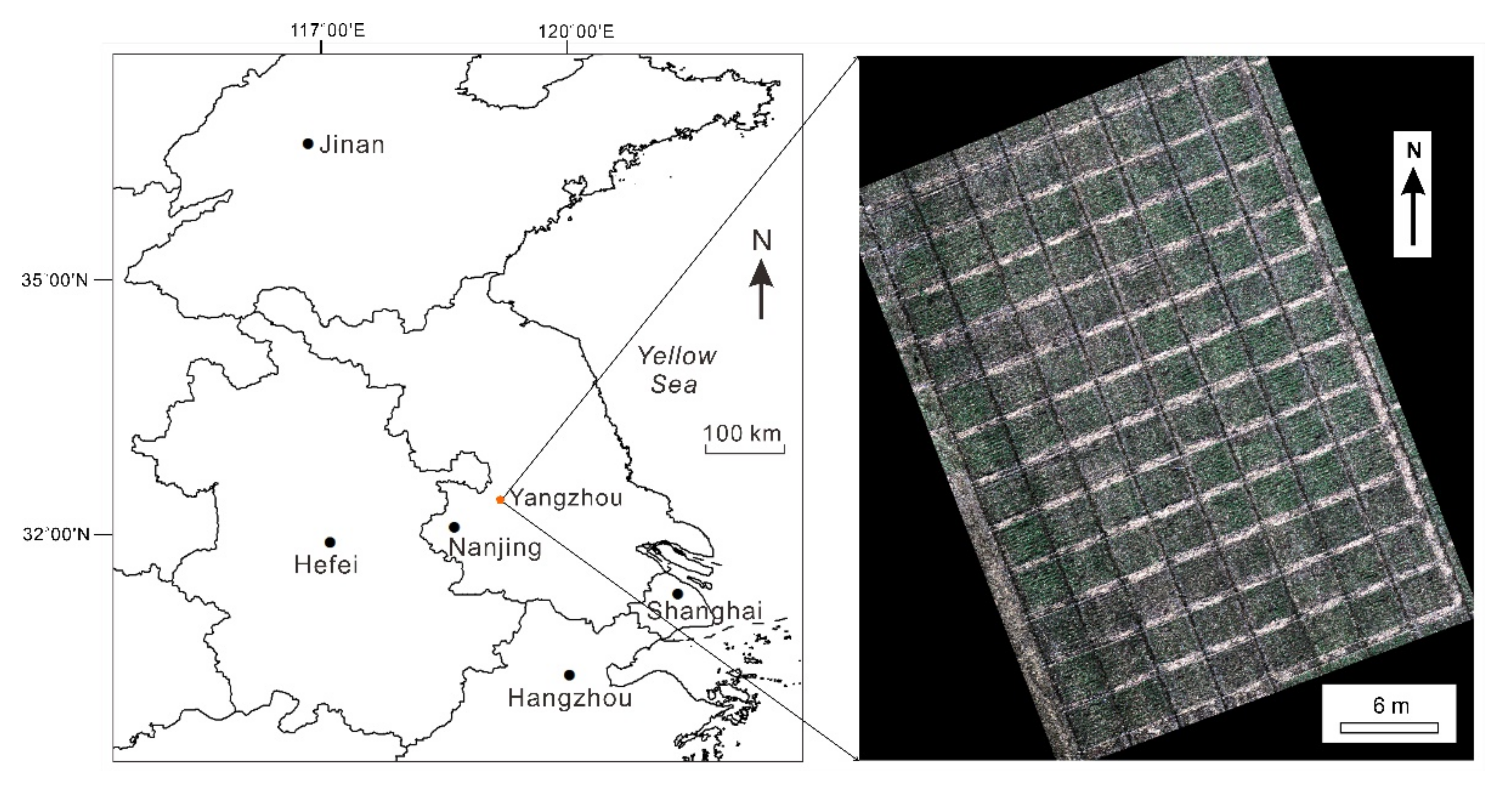
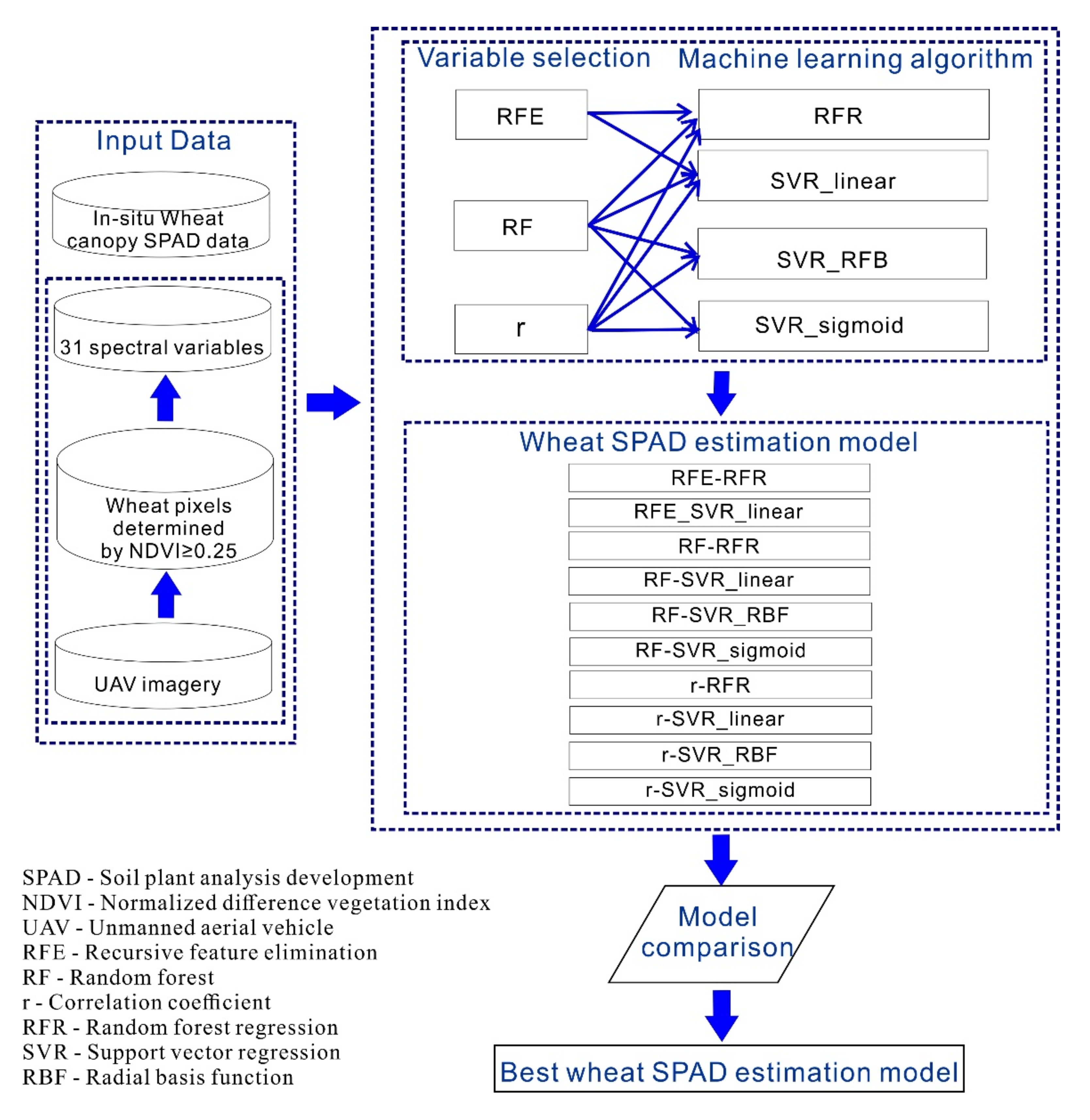
29], or other regression models. Nevertheless, there have been few previous studies that used variable selection in remote sensing of vegetation chlorophyll contents, although variable selection is critical. To fill this gap, the current study was designed to develop a good combination of variable selection methods with machine learning algorithms that can accurately estimate SPAD of wheat canopy at the overwintering stage, by comparative analysis. This study was based on the unmanned aerial vehicle (UAV) technology because the wheat variety screening experiments required high spatial resolution imagery.

2. Materials and Methods

2.1. Experimental Site and Experimental Design

The experiment was conducted at the Shatou Agricultural Experimental Farm located in Yangzhou, Jiangsu, China (32°18′39.96″N, 119°32′45.34″E) during the 2020/2021 wheat growing season (Figure 1). In total, 24 winter wheat varieties were sown under four rates of nitrogen fertilization through top-dressing (i.e., N0: 0 kg ha−1, N210: 210 kg ha−1, N270: 270 kg ha−1, and N330: 330 kg ha−1 pure nitrogen) on 15 November 2020, which was 10 days later than the local normal date for seed sowing. There were 96 plots in this experiment, and the size of each plot was 3 m long and 3 m wide. Each plot received the same irrigation and field managements.
The 24 winter wheat varieties are listed in Table 1. They had different optimal growth habits [30].

2.2. Data Acquisition

2.2.1. UAV Imagery Acquisition

The imagery of all plots in the experimental site was collected by the Phantom 4 Multispectral UAV (SZ DJI Technology Co.; Shenzhen, China) under clear weather conditions on 13 January 2021, at the overwintering stage of the winter wheat. The UAV was designed for precision agriculture equipped with a real-time kinematic (RTK) module capable of increasing the accuracy of Global Positioning System (GPS) location data.
Utilizing a gimbal with a 6-camera array, the UAV carried a RGB camera as well as a five-single-sensor camera that captured 2MP images in blue (450 nm ± 16 nm), green (560 nm ± 16 nm), red (650 nm ± 16 nm), red edge (730 nm ± 16 nm), and NIR (840 nm ± 26 nm) spectral regions. This study only used the images acquired by the five single sensors.
A gray gradient calibration panel, having 10 calibration plates with different gray gradients, was placed on the ground while the UAV was flying, for reflectivity correction [31]. The reflectance of these plates were spectrally measured in situ using an Analytical Spectral Device (ASD) FieldSpec® 3 Full-Range spectroradiometer (Analytical Spectral Devices, Inc.; Boulder, CO, USA).
The flight routes were designed using the software of the ground station (DJI GS PRO). Both the forward and side overlaps were set at 80%. The flight was conducted at 10:00 AM local time. The flight speed was fixed at 3 m s−1, and the flight altitude above ground level (AGL) was 15 m, which returned a spatial image resolution (i.e., ground sample distance) of 0.59 cm.

2.2.2. SPAD Measurements

SPAD values of wheat leaves were measured in situ in each plot using a non-destructive and portable SPAD-502plus handheld chlorophyll meter (Minolta Camera Co.; Osaka, Japan) immediately after UAV overpass. Within each plot, 10 leaves of the top layer were randomly selected. For each selected leaf, SPAD readings were recorded at one, three, and five sixths of leaf length of the leaf, and then the average was calculated and used for this leaf. The SPAD readings of the 10 selected leaves were then averaged to represent the plot.

2.3. Machine Learning Regression Algorithms Used

As mentioned above, RFR, SVR, and ANN are most frequently used for agricultural remote sensing [21], but ANN is not as practical as RFR and SVR [20]. Hence, this study employed RFR and SVR in wheat canopy SPAD estimation.

2.3.1. Random Forest Regression (RFR)

The random forest (RF) model is a classification or regression tree-based machine learning method proposed by Breiman [32]. The RF model uses bootstrap resampling methods to extract multiple bootstrap datasets from the original training dataset, develops a decision tree for each bootstrap dataset, and then combines these multiple parallel decision trees into a single RF model for prediction. The final prediction is obtained by applying a majority voting decision mechanism to the output of all individual decision trees. Stochasticity is introduced by the bootstrap strategy, which improves the resistance of the RF to overfitting [33]. When RF is used for regression, it is referred to as random forest regression (RFR). For RFR models, parameter tuning is required to optimize its two main parameters, namely the number of trees to grow in the forest (ntree) and the number of randomly selected predictor variables at each node (mtry) [34].

2.3.2. Support Vector Regression (SVR)

A support vector machine (SVM) or its regression version, support vector regression (SVR), is a supervised machine learning algorithm, which is powerful and flexible for classification and regression [35]. Using an optimal kernel, SVM maps the input data into different classes in a hyperplane in multidimensional space in an iterative manner until it finds a maximum marginal hyperplane, in which the differences among classes are maximized so as to minimize the error of classification [34].
Among the model parameters of SVR, gamma (kernel parameter) and C (penalty coefficient) have great influences on the estimation results, so they should be optimized through parameter tuning [17,27,36]. In addition, the kernels of linear, radial basis function (RBF) and sigmoid are commonly used; they were applied and tested in this study.

2.4. Methodology

2.4.1. UAV Image Processing and Index Extraction

The acquired UAV images were imported into the DJI Terra software to generate a digital surface model (DSM) and an orthomosaic image of the experimental plots in GeoTIFF format with UTM projection. The DN values were extracted from the orthomosaic image using the Environment for Visualizing Images (ENVI) software (ITT Exelis; Boulder, CO, USA) for each calibration plate, and then regression relationships between the DN values and their reflectance values were constructed for each of the five bands. Based on these regression relationships, DNs were converted to reflectance using the simplified empirical line approach proposed by Wang and Myint [37].
Then, the reflectance values at the blue, green, red, red edge, and NIR bands were extracted for each pixel in the entire UAV image of the experimental site. These reflectance values were used to further calculate 26 spectral indices. These spectral indices were often used to estimate crop chlorophyll contents and monitor crop growth status in the literature. In this study, a total of 31 variables, including 26 spectral indices and reflectance of five single bands, were used to develop a machine learning-based model to estimate SPAD values of wheat canopy. These 31 spectral variables and related computation formulas are listed in Table 2.
In general, the pixels with normalized difference vegetation index (NDVI) values of 0.2–0.3 were mixed pixels of non-vegetation and vegetation [55,56,57]. A careful visual check of the image revealed that the NDVI value of 0.25 could better discriminate wheat from soil, so the pixels with NDVI values lower than 0.25 were masked out in this study. Thus, the 31 variables were extracted and averaged as the variable values of the plot, respectively.

2.4.2. Variable Selection

The variable selection method of recursive feature elimination (RFE) starts working by searching a subset of variables from all variables in the training dataset, removes the least important variables, and then uses the remaining variables to refit the base model [27,58]. This process is repeated until a specific number of variables are retained, and the order in which variables are eliminated in this process is the ranking of the variables. This study tested using RFR and linear kernel SVR as a base model to conduct the RFE method, respectively. For RFE, its base model cannot be RBF kernel-based or sigmoid kernel-based SVR models [59].
RF is a fast and efficient machine learning algorithm, even when dealing with noisy variables [26]. RF is also a variable selection method [60]. It provides an easy way to assess variable importance. As a decision tree-based machine learning algorithm, RF can output a feature importance attribute; hence, all variables can be ranked in order of their own importance values calculated in the process of RF modeling [26].
The Pearson correlation coefficient (r) indicates a linear correlation between a predictor variable and a target variable, and its value ranges between −1 and 1. The predictor variables with higher absolute value of r have stronger linear correlation with the target variable, and hence they are selected prior to those predictor variables with lower absolute value of r in the variable selection method of Pearson correlation coefficient (r).
This study employed RFE, RF, and r to select variables. They are also most commonly used in previous studies [27].

2.4.3. Modeling, Cross Validation, and Performance Assessment

The 31 spectral variables (Table 2) were employed for feature selection after being standardized using the standardized method of StandardScaler. The standardized method was from a Python library named “sklearn.preprocessing” [61].
To obtain the most effective model for estimating the SPAD of wheat canopy through comparative analysis, this study combined three variable selection methods with four machine learning algorithms, resulting in 10 SPAD estimation models, which included seven SVR models (i.e., RFE-SVR_linear, RF-SVR_linear, RF-SVR_RBF, RF-SVR_sigmoid, r-SVR_linear, r-SVR_RBF, and r-SVR_sigmoid) and three RFR models (i.e., RFE-RFR, RF-RFR, and r-RFR).
Parameter tuning plays an important role in achieving the best performance of machine learning-based models [35], and this study combined grid search techniques with cross-validation to find the best parameter values. For each of the 10 models, the optimal number of variables (n_features_to_select) was determined by searching values from 1 to 31 in an interval of 1 and selecting the number of variables that achieves the best cross-validation accuracy.
To optimize the RFR models, the number of input variables was used as the mtry value. Nine values (i.e., 50, 100, 200, 700, 1000, 1100, 1200, 1300, and 2000 trees) were used as the ntree value, respectively, and the ntree value resulting in the best cross-validation accuracy was selected as the optimal ntree.
To optimize the SVR models, the penalty C was evaluated using values from 1 to 500 with an interval of 1, and the parameter gamma was searched with values from 0.0001 to 0.01, with an interval of 0.0002. The C and gamma achieving the best cross-validation accuracy were selected as the optimal parameter values.
Figure 2 summarizes the methodology used. The entire process of variable selection, modeling, cross-validation, and performance evaluation was performed with a desktop computer using a Python program written for this study based on the Scikit-learn package [62], which is an open source Python module. The optimal values of the above mentioned key parameters such as n_features_to_select, mtry, ntree, C, and gamma were determined simultaneously according to the SPAD estimation accuracy, using cross-validation and the grid search strategy. Correspondingly, the SPAD estimation model with the highest estimation accuracy was considered as the optimum SPAD estimation model of wheat canopy.
Among various cross-validation techniques, this study selected the leave-one-out cross-validation (LOOCV). The LOOCV [35] selects one sample each time for validation and uses all the other samples to develop a model, and then uses the selected one sample to calculate the estimation errors until all samples are involved in the cross validation. The LOOCV can assess the generalization capability of the models [35] and eliminate overfitting [63], and it was used to evaluate the model reliability and stability.
The accuracy of models was evaluated by achieved R2, RMSE, and relative RMSE (RRMSE) in SPAD estimation. The LOOCV results of R2, RMSE, and RRMSE were calculated following Wang and Lu [64].
In general, a higher R2 value and lower RMSE and RRMSE values indicate better model performance [65]. In addition, this study also calculated the ratio of percentage deviation (RPD) to assess the predictive capability of models. RPD is the ratio of the standard deviation of the measured values to the RMSE of the cross-validation [66]. According to Viscarra Rossel et al. [67], RPD < 1.4 indicates very poor or poor estimations, 1.4 ≤ RPD < 1.8 indicates fair estimations, 1.8 ≤ RPD < 2.0 indicates good estimations, 2.0 ≤ RPD < 2.5 indicates very good estimations, and RPD ≥ 2.5 indicates excellent estimations.

3. Results

3.1. Descriptive Statistics of Measured Wheat Canopy SPAD Values

Table 3 displays the variation of SPAD values of wheat canopy, which were in situ measured from all the 96 plots in the late-sown wheat variety screening experiment. SPAD values ranged from 30.89 to 44.82. The mean SPAD was 38.09 with a standard deviation of 3.46.
The 96 plots were divided to four groups (i.e., N0 plots, N210 plots, N270 plots, and N330 plots) according to their rates of nitrogen fertilization (i.e., 0, 210, 270, and 330 kg ha−1 pure nitrogen), respectively. Table 3 demonstrates that the mean SPAD values increased significantly from 33.80 to 38.31 from N0 plots to N210 plots, and then increased slightly to 39.73 of N270 plots and to 40.54 of N330 plots. In addition, the standard deviation of N0 plots was also smaller than those of N210 plots, N270 plots, and N330 plots.

3.2. Spectral Characteristics of Wheat Canopy SPAD Values

The correlation coefficients between 31 UAV-derived variables and SPAD values of wheat canopy were calculated (Figure 3). The five single bands were not well correlated with the SPAD. The absolute r value of the near-infrared band was only 0.404, and the absolute r values of the other four were below 0.270.
For variables that included only the visible bands, their absolute r values were not higher than 0.431. For variables that included the near-infrared band but not the red edge band, their absolute r values were between 0.404 and 0.595. For variables that included the red edge band, their absolute r values were between 0.268 and 0.772.
Of the 31 variables, only three had absolute r values higher than 0.700 (Red edge chlorophyll index (CIRE): 0.772, MERIS terrestrial chlorophyll index (MTCI): 0.748, and Modified chlorophyll absorption reflectance index 1 (MCARI1): 0.728). They are all vegetation indices related to chlorophyll. In contrast, all the other 28 variables had absolute r values below 0.600.
To compare spectral curves for varying SPAD values, this study averaged the SPAD and spectral reflectance values for the four groups (i.e., N0 plots, N210 plots, N270 plots, and N330 plots). As illustrated in Figure 4, the spectral reflectance of the four groups had similar variations with increasing wavelength, although they had different mean SPAD values. Moreover, in general, reflectance increases with increasing SPAD, especially in the red edge and near-infrared regions.

3.3. SPAD Inversion Models

For each model, the best model parameters were retrieved using the grid search technique, according to the resultant lowest RMSE by the LOOCV. These optimal parameters are listed in Table 4.
The selected optimal variables of each model are listed in Table 5. The optimal variables were quite different among the 10 models. MCARI1 was the only variable that was commonly selected by all 10 models. The three RFR models had three common selected variables (i.e., MCARI1, MTCI, and CIRE). The seven SVR models had five common selected variables (i.e., MCARI1, VARI, GI, RGRI, and MCARI).

3.4. Performance of SPAD Inversion Models

Table 6 displays the accuracies of the 10 models for estimating the SPAD. RF-SVR_sigmoid achieved the highest estimation accuracy (Optimal number of variables = 27, R2 = 0.754, RPD = 2.017, RMSE = 1.716, and RRMSE = 4.504%), followed by r-SVR_sigmoid (Optimal number of variables = 31, R2 = 0.743, RPD = 1.973, RMSE = 1.754, and RRMSE = 4.605%), and RFE-SVR_linear (Optimal number of variables = 7, R2 = 0.730, RPD = 1.926, RMSE = 1.797, and RRMSE = 4.718%).
To further analyze the modeling accuracy, Figure 5 presents the scatterplots of the measured SPAD against the estimated SPAD by the LOOCV, when the three models that achieved the best estimation performance were applied. For all three models, the data points are well distributed along the 1:1 relationship, demonstrating good agreements between the measured and estimated SPAD values.
This study compared the accuracies of the selected best model, RF-SVR_sigmoid, in estimating wheat canopy SPAD for plots under four different rates of nitrogen fertilization (Table 7). RMSE ranged from 1.500 (N0 plots) to 2.017 (N210 plots), and RRMSE ranged from 4.054% (N270 plots) to 5.265% (N210 plots).
This study also compared the SPAD estimation accuracies of the RF-SVR_sigmoid model for wheat varieties that have three different optimal growth habits (Table 8). RMSE ranged from 1.486 to 2.088, and RRMSE ranged from 3.866% to 5.176%, with the lowest in the N270 plots and the highest in the N210 plots. The semi-winterness varieties had the lowest RMSE and RRMSE, followed by the springiness varieties and the weak springiness varieties.

4. Discussion

4.1. Optimal SPAD Estimation Model for Late-Sown Winter Wheat Variety Screening

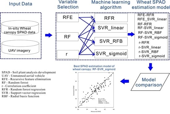
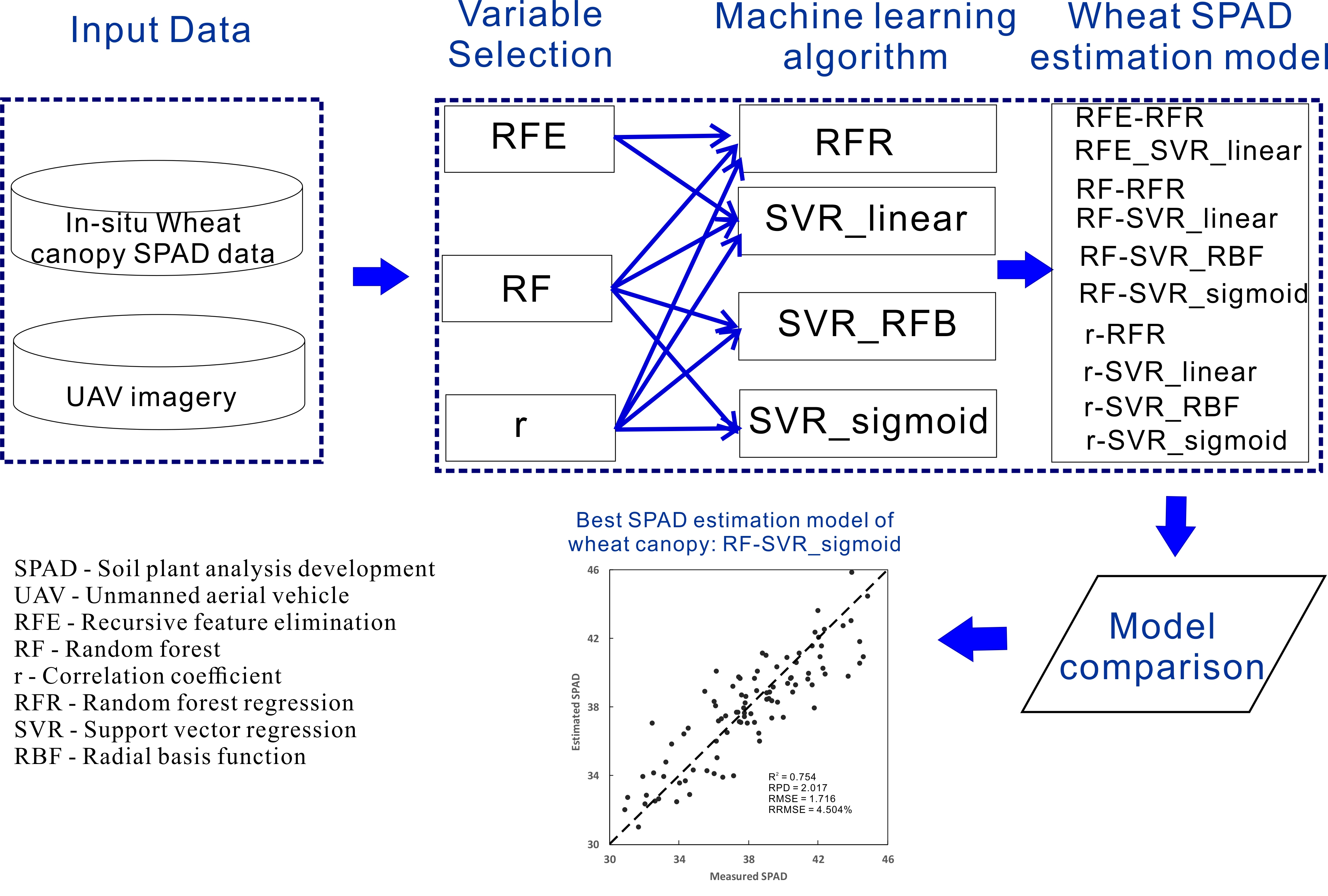
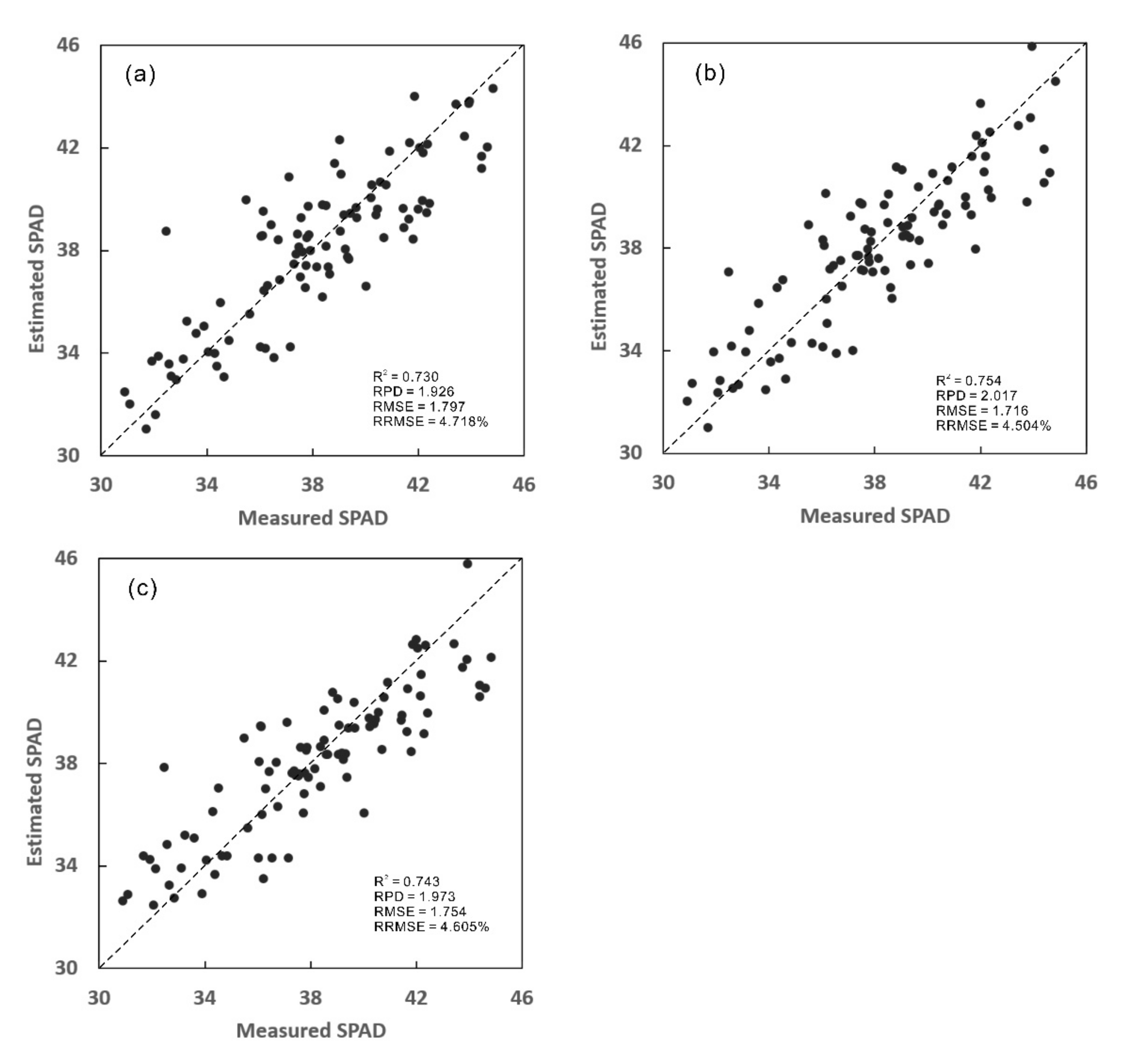
This study involved up to 24 wheat varieties, four rates of nitrogen fertilization, and 96 plots in a variety screening experiment, which resulted in a very complex relationship between wheat canopy SPAD values and spectral variables. Therefore, this study investigated the feasibility of using machine learning-based models rather than conventional ones to estimate SPAD of wheat canopy from UAV data at the overwintering stage. Seven SVR models and three RFR models were developed, cross-validated, and compared. Of these 10 models, the RF-SVR_sigmoid model, which was constructed by combining the RF variable selection method and the sigmoid kernel-based SVR algorithm, was identified as the best model. It achieved the highest accuracy in estimating SPAD values by the LOOCV (R2 = 0.754, RPD = 2.017, RMSE = 1.716, and RRMSE = 4.504%). According to Viscarra Rossel et al. [67], the model of RF-SVR_sigmoid (RPD = 2.017) achieved very good SPAD estimation of wheat canopy. In contrast, r-SVR_sigmoid (RPD = 1.973) and RFE-SVR_linear (RPD = 1.926) only produced good estimation, but their RPD values were very close to 2.
Despite the fact that the study involved up to 24 different wheat varieties, the newly developed RF-SVR_sigmoid model was able to achieve high accuracy in SPAD estimation. Moreover, the model worked well for both plots under different rates of nitrogen fertilization and plots with springness, weak springness, and semi-winterness varieties. It is particularly important for wheat variety screening that the developed model can be used for all the wheat varieties involved, considering that the best varieties are usually screened from a large number of varieties. In contrast, most previous studies of SPAD remote sensing involved only a single variety or a very small number of varieties, which is not suitable for variety screening [68,69,70].

4.2. Model Performance Comparison

A comparison of the seven SVR models (i.e., RFE-SVR_linear, RF-SVR_linear, RF-SVR_RBF, RF-SVR_sigmoid, r-SVR_linear, r-SVR_RBF, and r-SVR_sigmoid) with the three RFR models (i.e., RFE-RFR, RF-RFR, and r-RFR) finds that even the worst SVR model (i.e., r-SVR_linear) could produce better SPAD estimates (R2 = 0.710, RPD = 1.857, RMSE = 1.864, and RRMSE = 4.893%) than the best RFR model (i.e., RFE-RFR) (R2 = 0.640, RPD = 1.666, RMSE = 2.077, and RRMSE = 5.452%). In addition, the improvement in estimation accuracy was even greater when the best SVR model (i.e., the RF-SVR_sigmoid model) (R2 = 0.754, RPD = 2.017, RMSE = 1.716, and RRMSE = 4.504%) was compared with the best RFR model of RFE-RFR.
Given the encouraging performances of the SVR, however, it is too early to say that the SVR model always outperforms the RFR model in estimating vegetation chlorophyll content. For the estimation of other agricultural variables, some studies had reported that the RFR model outperformed the SVR model. For example, Osco et al. [71] noted that, using UAV multispectral images, the RFR model was able to predict leaf nitrogen content (LNC) of maize more accurately than the SVR model. Similarly, Zha et al. [65] reported that the RFR algorithm performed better than the SVR and ANN models in estimating the nitrogen nutrient index (NNI) of rice from drone data.
Yang et al. [22] indicated that appropriate kernels could better avoid overfitting. The RBF kernel was considered to be the most frequently used kernel function [72]. Some previous studies (e.g., Ahmad et al. [73]; Chen and Hay [74]) reported that the RBF kernel performed better relative to linear and sigmoid kernels. However, this study found that among the seven SVR models, the two sigmoid kernel-based SVR models performed the best, followed by the RFE-SVR_linear model, while the two RBF kernel-based SVR models produced lower accuracy. Hence, the sigmoid kernel seemed more appropriate for SVR in terms of SPAD estimation.
In addition, although the RFE-SVR_linear model was not as good as the two SVR models with sigmoid kernel, its SPAD estimation was also good. Moreover, the linear kernel–based SVR model runs much faster than the RBF kernel-based SVR model [75].

4.3. Influence of Different Variable Selection Methods on Model Estimation Performance

Little previous research has investigated employing variable selection in machine learning-based remote sensing of vegetation chlorophyll contents. This research found that the optimal combination of variable selection methods and machine learning algorithms could produce more accurate SPAD estimation of wheat canopy. Among various combinations of three variable selection methods and four machine learning algorithms, the combination of RF and SVR_sigmoid demonstrates the best capability of SPAD estimation.
In this study, the RFR and SVR_linear models using the RFE variable selection method provided overall higher R2 and more robust results than the RFR and SVR_linear models using RF or r variable selection methods. In addition, the number of optimal variables selected using RFE was much smaller than those selected using RF or r. Results from this study disagree with the superiority of RF over RFE as a variable selection method, as reported by Chen et al. [27]. More research should be conducted to further evaluate these variable selection methods in agricultural remote sensing.
Using RF to select the optimal variables resulted in more accurate SPAD estimates compared with using the r variable selection method (Table 6). However, the differences caused by using different variable selection methods are not as large as those caused by using different machine learning algorithms.
Three models produced the lowest RMSE and RRMSE (i.e., RFE-SVR_linear, RF-SVR_sigmoid, and r-SVR_sigmoid), as displayed in Table 6. They had seven common optimal variables (i.e., green, VARI, GI, RGRI, RI, MCARI1, and MCARI) (Table 5). This indicates that the seven variables are particularly important for accurate estimation of wheat canopy SPAD. The seven variables were selected from the 31 variables (Table 2) that included 10 variables (i.e., NPCI, GCVI, CVI, MCARI1, MCARI, MTCI, NCARI, TCI, TCARI, and CIRE) proposed and widely used for monitoring chlorophyll or SPAD in previous studies [16,40,54]. It is a bit surprising that, among the 10 variables, only two (i.e., MCARI1 and MCARI) are commonly selected by the three best SPAD estimation models in this study.

4.4. Limitations and Future Research

Although this preliminary study proposed a promising method for SPAD monitoring, there were still some limitations. This study found that the NDVI value of 0.25 could discriminate wheat from soil. When the new method is applied on other dates or on other farms, the threshold should be determined through a very careful visual check of the entire image.
Besides chlorophyll content, canopy reflectance is also sensitive to other influencing factors, such as canopy structure and leaf area index [9,15]. The error in the SPAD estimation of the RF-SVR_sigmoid model could be partially attributed to the omission of these influencing factors. Considering these influencing factors may further improve the SPAD estimation accuracies in future research.
This study applied 96 plots, and future research will employ a larger data base. In addition, this study involved 18 springness wheat varieties, and in contrast it involved only two weak springness varieties and four semi-winterness varieties. Hence, the wheat variety shares should be balanced in future research.
This study used only data from one growing season (i.e., the overwintering growth stage). Future research should collect data at more growth stages. In addition, this study involved only a single year, but variety screening often needs multiple-year experiments. Hence, the conclusions drawn in this study should be further evaluated in future studies with data from multiple growth stages and more years on various experimental farms.

5. Conclusions

This study demonstrates that the combination of different variable selection methods with different machine learning algorithms can impact the estimation accuracy quite significantly. The optimal combination of variable selection methods and machine learning algorithms could produce more accurate SPAD estimation. The newly developed RF-SVR_sigmoid model, which is the combination of the RF variable selection method and the sigmoid kernel-based SVR algorithm, can accurately estimate SPAD of wheat canopy at the overwintering stage. The results of LOOCV prove that the estimation is very good, and the newly developed model can be used for all 24 wheat varieties involved.
The spectral data used in this study were acquired using a multispectral UAV. This study demonstrates the potential of UAV remote sensing for late-sown winter wheat variety screening. Use of UAVs is more efficient, time-saving, and convenient than traditional in situ measurements of SPAD. In comparison to satellite remote sensing, use of low-altitude UAVs is more flexible, and it provides imagery with much higher spatial resolutions, which is necessary considering the size of plots in variety screening experiments. The widespread use of UAV technology nowadays allows a fast and accurate monitoring of wheat canopy SPAD at the overwintering stage using the newly developed RF-SVR_sigmoid model, and this is critical for late-sown winter wheat variety screening.

Author Contributions

Conceptualization, J.W.; formal analysis, J.W.; funding acquisition, J.W., Z.H. and C.T.; investigation, J.W., Q.Z., C.L., T.Z., J.D., Y.X., L.Z., W.W. and G.Z.; methodology, J.W. and Q.Z.; supervision, J.W. and Z.H.; visualization, J.W. and Q.Z.; writing—original draft, J.W. and J.S.; writing—review and editing, J.W. and J.S. All authors have read and agreed to the published version of the manuscript.

Funding

This research was funded by the Science and Technology Programme of Yangzhou City, Jiangsu, China (project no. YZ2021031), the Key Research and Development Program of Jiangsu Province, China (project no. BE2020319), Yangzhou University High-end Talent Support Plan (2018), the Priority Academic Program Development of Jiangsu Higher Education Institutions (PAPD), China, the National Natural Science Foundation of China (project no. 32071902), and the Interdisciplinary Project of Yangzhou University Crop Science Special Zone (project no. yzuxk202007).

Acknowledgments

Special thanks to Quan Yin, Agricultural College of Yangzhou University, Jiangsu, China for his kind help in the process of preparing for field surveys.

Conflicts of Interest

The authors declare no conflict of interest.

References

  1. Gao, D.; Wang, H.; Liu, Q.; Zhu, D.; Zhang, X.; Lu, G.; Zhang, X.; Jiang, W.; Li, M. Breeding of New Wheat Varieties with Early Maturity and High Yield under Late Sowing. Sci. Agric. Sin. 2019, 52, 2379–2390, (In Chinese with English Abstract). [Google Scholar]
  2. Gao, D.; Zhang, X.; Kang, J.; Bie, T.; Zhang, B.; Zhang, X.; Cheng, S. Negative effects of late sowing on wheat production in middle and lower reaches of Yangtze River Valley and breeding strategies. J. Triticeae Crop. 2014, 34, 279–283, (In Chinese with English Abstract). [Google Scholar]
  3. Li, C.; Yang, J.; Zhang, Y.; Yao, M.; Zhu, X.; Guo, W. Retrieval Effects of Remedial Fertilizer after Freeze Injury on Wheat Yield and Its Mechanism at Tillering Stage. Sci. Agric. Sin. 2017, 50, 1781–1791, (In Chinese with English Abstract). [Google Scholar]
  4. Zhang, S.; Zhao, G.; Lang, K.; Su, B.; Chen, X.; Xi, X.; Zhang, H. Integrated satellite, unmanned aerial vehicle (UAV) and ground inversion of the SPAD of winter wheat in the reviving stage. Sensors 2019, 19, 1485. [Google Scholar] [CrossRef] [Green Version]
  5. Gitelson, A.A.; Merzlyak, M.N. Remote sensing of chlorophyll concentration in higher plant leaves. Adv. Space Res. 1998, 22, 689–692. [Google Scholar] [CrossRef]
  6. Li, J.; Feng, Y.; Mou, J.; Xu, G.; Luo, Q.; Luo, K.; Huang, S.; Shi, X.; Guan, Z.; Ye, Y.; et al. Construction and Application Effect of the Leaf Value Model Based on SPAD Value in Rice. Sci. Agric. Sin. 2017, 50, 4714–4724, (In Chinese with English Abstract). [Google Scholar]
  7. Haboudane, D.; Tremblay, N.; Miller, J.R.; Vigneault, P. Remote estimation of crop chlorophyll content using spectral indices derived from hyperspectral data. IEEE Trans. Geosci. Remote. Sens. 2008, 46, 423–437. [Google Scholar] [CrossRef]
  8. Croft, H.; Chen, J.M.; Zhang, Y. The applicability of empirical vegetation indices for determining leaf chlorophyll content over different leaf and canopy structures. Ecol. Complex. 2014, 17, 119–130. [Google Scholar] [CrossRef]
  9. Wu, C.Y.; Niu, Z.; Tang, Q.; Huang, W.J. Estimating chlorophyll content from hyperspectral vegetation indices: Modeling and validation. Agric. For. Meteorol. 2008, 148, 1230–1241. [Google Scholar] [CrossRef]
  10. Hunt, E.R.; Doraiswamy, P.C.; Mcmurtrey, J.E.; Daughtry, C.S.T.; Perry, E.M.; Akhmedov, B. A visible band index for remote sensing leaf chlorophyll content at the canopy scale. Int. J. Appl. Earth Obs. 2013, 21, 103–112. [Google Scholar] [CrossRef] [Green Version]
  11. Daughtry, C.S.T.; Walthall, C.L.; Kim, M.S.; Brown de Colstoun, E.; McMurtrey, J.E., III. Estimating corn leaf chlorophyll concentration from leaf and canopy reflectance. Remote Sens. Environ. 2000, 74, 229–239. [Google Scholar] [CrossRef]
  12. Cao, Q.; Miao, Y.; Wang, H.; Huang, S.; Cheng, S.; Khosla, R.; Jiang, R. Non-Destructive Estimation of Rice Plant Nitrogen Status with Crop Circle Multispectral Active Canopy Sensor. Field Crops Res. 2013, 154, 133–144. [Google Scholar] [CrossRef]
  13. Dash, J.; Curran, P.J. The MERIS terrestrial chlorophyll index. Int. J. Remote Sens. 2004, 25, 5403–5413. [Google Scholar] [CrossRef]
  14. Moharana, S.; Dutta, S. Spatial variability of chlorophyll and nitrogen content of rice from hyperspectral imagery. ISPRS J. Photogramm. 2016, 122, 17–29. [Google Scholar] [CrossRef]
  15. Gitelson, A.A.; Vina, A.S.; Ciganda, V.N.; Rundquist, D.C. Remote estimation of canopy chlorophyll content in crops. Geophys. Res. Lett. 2005, 32, L08403. [Google Scholar] [CrossRef] [Green Version]
  16. Vincini, M.; Frazzi, E.; D’Alessio, P. A broad-band leaf chlorophyll vegetation index at the canopy scale. Precis. Agric. 2008, 9, 303–319. [Google Scholar] [CrossRef]
  17. An, G.; Xing, M.; He, B.; Liao, C.; Kang, H. Using machine learning for estimating rice chlorophyll content from in situ hyperspectral data. Remote Sens. 2020, 12, 3104. [Google Scholar] [CrossRef]
  18. Main, R.; Cho, M.A.; Mathieu, R.; O’Kennedy, M.M.; Ramoelo, A.; Koch, S. An investigation into robust spectral indices for leaf chlorophyll estimation. ISPRS J. Photogramm. 2011, 66, 751–761. [Google Scholar] [CrossRef]
  19. Jin, X.; Li, Z.; Feng, H.; Xu, X.; Yang, G. Newly combined spectral indices to improve estimation of total leaf chlorophyll content in cotton. IEEE J. Sel. Top. Appl. Earth Obs. Remote Sens. 2014, 7, 4589–4600. [Google Scholar] [CrossRef]
  20. Chlingaryan, A.; Sukkarieh, S.; Whelan, B. Machine learning approaches for crop yield prediction and nitrogen status estimation in precision agriculture: A review. Comput. Electron. Agric. 2018, 151, 61–69. [Google Scholar] [CrossRef]
  21. Ashapure, A.; Jung, J.; Chang, A.; Oh, S.; Yeom, J.; Maeda, M.; Maeda, A.; Dube, N.; Landivar, J.; Hague, S.; et al. Developing a machine learning based cotton yield estimation framework using multi-temporal UAS data. ISPRS J. Photogramm. 2020, 169, 180–194. [Google Scholar] [CrossRef]
  22. Yang, X.; Huang, J.; Wu, Y.; Wang, J.; Wang, P.; Wang, X.; Huete, A.R. Estimating biophysical parameters of rice with remote sensing data using support vector machines. Sci. China Life Sci. 2011, 54, 272–281. [Google Scholar] [CrossRef] [Green Version]
  23. Liu, H.; Li, M.; Zhang, J.; Gao, D.; Sun, H.; Yang, L. Estimation of chlorophyll content in maize canopy using wavelet denoising and SVR method. Int. J. Agric. Biol. Eng. 2018, 11, 132–137. [Google Scholar] [CrossRef] [Green Version]
  24. Cavallo, D.P.; Cefola, M.; Pace, B.; Logrieco, A.F.; Attolico, G. Contactless and non-destructive chlorophyll content prediction by random forest regression: A case study on fresh-cut rocket leaves. Comput. Electron. Agric. 2017, 140, 303–310. [Google Scholar] [CrossRef]
  25. Bolón-Canedo, V.; Sánchez-Maroño, N.; Alonso-Betanzos, A. Feature selection for high-dimensional data. Prog. Artif. Intell. 2016, 5, 65–75. [Google Scholar] [CrossRef]
  26. Hoa, P.V.; Giang, N.V.; Binh, N.A.; Hai, L.V.H.; Pham, T.D.; Hasanlou, M.; Bui, D.T. Soil salinity mapping using SAR Sentinel-1 data and advanced machine learning algorithms: A case study at Ben Tre Province 631 of the Mekong River Delta (Vietnam). Remote Sens. 2019, 11, 128. [Google Scholar] [CrossRef] [Green Version]
  27. Chen, L.; Xing, M.; He, B.; Wang, J.; Xu, M. Estimating soil moisture over winter wheat fields during growing season using machine-learning methods. IEEE J. Sel. Top. Appl. Earth Obs. Remote Sens. 2021, 14, 3706–3718. [Google Scholar] [CrossRef]
  28. Rasel, S.M.M.; Chang, H.C.; Ralph, T.J.; Saintilan, N.; Diti, I.J. Application of feature selection methods and machine learning algorithms for saltmarsh biomass estimation using Worldview-2 imagery. Geocarto Int. 2021, 36, 1075–1099. [Google Scholar] [CrossRef]
  29. Dang, A.T.N.; Nandy, S.; Srinet, R.; Luong, N.V.; Ghosh, S.; Kumar, A.S. Forest aboveground biomass estimation using machine learning regression algorithm in Yok Don National Park, Vietnam. Ecol. Inform. 2019, 50, 24–32. [Google Scholar] [CrossRef]
  30. Chen, S.; Wang, J.; Deng, G.; Chen, L.; Cheng, X.; Xu, H.; Zhan, K. Interactive effects of multiple vernalization (vrn-1)- and photoperiod (ppd-1)-related genes on the growth habit of bread wheat and their association with heading and flowering time. BMC Plant Biol. 2018, 18, 374. [Google Scholar] [CrossRef]
  31. Qiu, Z.; Ma, F.; Li, Z.; Xu, X.; Ge, H.; Du, C. Estimation of nitrogen nutrition index in rice from UAV RGB images coupled with machine learning algorithms. Comput. Electron. Agric. 2021, 189, 106421. [Google Scholar] [CrossRef]
  32. Breiman, L. Random forests. Mach. Learn. 2001, 45, 5–32. [Google Scholar] [CrossRef] [Green Version]
  33. Fu, P.; Meacham, K.; Guan, K.; Bernacchi, C.J. Hyperspectral leaf reflectance as proxy for photosynthetic capacities: An ensemble approach based on multiple machine learning algorithms. Front Plant Sci. 2019, 10, 730. [Google Scholar] [CrossRef]
  34. Forkuor, G.; Hounkpatin, O.K.; Welp, G.; Thiel, M. High resolution mapping of soil properties using remote sensing variables in South-Western Burkina Faso: A comparison of machine learning and multiple linear regression models. PLoS ONE 2017, 12, e0170478. [Google Scholar] [CrossRef]
  35. Adab, H.; Morbidelli, R.; Saltalippi, C.; Moradian, M.; Ghalhari, G. Machine learning to estimate surface soil moisture from remote sensing data. Water 2020, 12, 3223. [Google Scholar] [CrossRef]
  36. Lan, Y.; Huang, Z.; Deng, X.; Zhu, Z.; Tong, Z. Comparison of machine learning methods for citrus greening detection on UAV multispectral images. Comput. Electron. Agric. 2020, 171, 105234. [Google Scholar] [CrossRef]
  37. Wang, C.; Myint, S.W. A simplified empirical line method of radiometric calibration for small unmanned aircraft systems-based remote sensing. IEEE J. Sel. Top. Appl. Earth Obs. Remote Sens. 2015, 8, 1876–1885. [Google Scholar] [CrossRef]
  38. Gholizadeh, A.; Saberioon, M.; Viscarra Rossel, R.A.; Boruvka, L.; Klement, A. Spectroscopic measurements and imaging of soil colour for field scale estimation of soil organic carbon. Geoderma 2020, 357, 113972. [Google Scholar] [CrossRef]
  39. Gitelson, A.A.; Viña, A.; Arkebauer, T.J.; Rundquist, D.C.; Keydan, G.; Leavitt, B. Remote estimation of leaf area index and green leaf biomass in maize canopies. Geophys. Res. Lett. 2003, 30, 1248. [Google Scholar] [CrossRef] [Green Version]
  40. Penuelas, J.; Gamon, J.A.; Fredeen, A.L.; Merino, J.; Field, C.B. Reflectance indices associated with physiological changes in nitrogen- and water-limited sunflower leaves. Remote Sens. Environ. 1994, 48, 135–146. [Google Scholar] [CrossRef]
  41. Woebbecke, D.M.; Meyer, G.E.; Von Bargen, K.; Mortensen, D.A. Color indices for weed identification under various soil, residue, and lighting conditions. Trans. ASAE 1995, 38, 259–269. [Google Scholar] [CrossRef]
  42. Zarco-Tejada, P.J.; Berjón, A.; López-Lozano, R.; Miller, J.R.; Martín, P.; Cachorro, V.; González, M.R.; de Frutos, A. Assessing vineyard condition with hyperspectral indices: Leaf and canopy reflectance simulation in a row-structured discontinuous canopy. Remote Sens. Environ. 2005, 99, 271–287. [Google Scholar] [CrossRef]
  43. Xu, Y.; Wang, X.; Sun, H.; Wang, H.; Zhan, Y. Study of monitoring maize leaf nutrition based on image processing and spectral analysis. In The World Automation Congress; IEEE: Piscataway, NJ, USA, 2010; pp. 465–468. [Google Scholar]
  44. Barron, V.; Torrent, J. Use of the Kubelka-Munk theory to study the influence of iron oxides on soil colour. J. Soil Sci. 1986, 37, 499–510. [Google Scholar] [CrossRef]
  45. Gitelson, A.A.; Kaufman, Y.J.; Merzlyak, M.N. Use of a green channel in remote sensing of global vegetation from EOS-MODIS. Remote Sens. Environ. 1996, 58, 289–298. [Google Scholar] [CrossRef]
  46. Rouse, J.W.; Haas, R.H.; Schell, J.A.; Deering, D.W.; Harlan, J.C. Monitoring the Vernal Advancements and Retrogradation of Natural Vegetation; Final Report; NASA/GSFC: Greenbelt, MN, USA, 1974; pp. 1–137. [Google Scholar]
  47. Rondeaux, G.; Steven, M.; Baret, F. Optimization of Soil-Adjusted Vegetation Indices. Remote Sens. Environ. 1996, 55, 95–107. [Google Scholar] [CrossRef]
  48. Huete, A. A soil-adjusted vegetation index (SAVI). Remote Sens. Environ. 1988, 25, 295–309. [Google Scholar] [CrossRef]
  49. Pearson, R.L.; Miller, L.D. Remote mapping of standing crop biomass for estimation of the productivity of the shortgrass prairie. In Proceedings of the Eighth International Symposium on Remote Sensing of Environment, Ann Arbor, MI, USA, 2–6 October 1972; pp. 1357–1381. [Google Scholar]
  50. Tucker, C.J. Red and photographic infrared linear combinations for monitoring vegetation. Remote Sens. Environ. 1979, 8, 127–150. [Google Scholar] [CrossRef] [Green Version]
  51. Richardson, A.J.; Wiegand, C.L. Distinguishing vegetation from soil background information. Photogramm. Eng. Remote Sens. 1978, 43, 1541–1552. [Google Scholar]
  52. Perry, C.R.; Lautenschlager, L.F. Functional equivalence of spectral vegetation indices. Remote Sens. Environ. 1984, 14, 169–182. [Google Scholar] [CrossRef]
  53. Wei, Q.; Zhang, B.; Wei, Z.; Han, X.; Duan, C. Estimation of canopy chlorophyll content in winter wheat by UAV multispectral remote sensing. J. Triticeae Crop. 2020, 40, 365–372, (In Chinese with English Abstract). [Google Scholar]
  54. Haboudane, D.; Miller, J.R.; Tremblay, N.; Zarco-Tejada, P.J.; Dextraze, L. Integrated narrow-band vegetation indices for prediction of crop chlorophyll content for application to precision agriculture. Remote Sens. Environ. 2002, 81, 416–426. [Google Scholar] [CrossRef]
  55. Wang, J.J.; Zhang, Y.; Bussink, C. Unsupervised Multiple Endmember Spectral Mixture Analysis-Based Detection of Opium Poppy Fields from an EO-1 Hyperion Image in Helmand, Afghanistan. Sci. Total Environ. 2014, 476–477, 1–6. [Google Scholar] [CrossRef] [PubMed]
  56. Tsai, F.; Lin, E.K.; Yoshino, K. Spectrally segmented principal component analysis of hyperspectral imagery for mapping invasive plant species. Int. J. Remote Sens. 2007, 28, 1023–1039. [Google Scholar] [CrossRef]
  57. Noujdina, N.V.; Ustin, S.L. Mapping downy brome (Bromus tectorum) using multidate AVIRIS data. Weed Sci. 2008, 56, 173–179. [Google Scholar] [CrossRef]
  58. Han, L.; Yang, G.J.; Dai, H.Y.; Xu, B.; Yang, H.; Feng, H.K.; Li, Z.H.; Yang, X.D. Modeling maize above-ground biomass based on machine learning approaches using UAV remote-sensing data. Plant Methods 2019, 15, 10. [Google Scholar] [CrossRef] [PubMed] [Green Version]
  59. Code Pioneer. Error: “The Classifier Does Not Expose ‘Coef_’ or ‘Feature_Importances_’”. Available online: https://www.codeleading.com/article/41762717838/ (accessed on 26 June 2021).
  60. Ghosh, S.M.; Behera, M.D. Aboveground biomass estimation using multi-sensor data synergy and machine learning algorithms in a dense tropical forest. Appl. Geogr. 2018, 96, 29–40. [Google Scholar] [CrossRef]
  61. Scikit-Learn Developers. Sklearn.preprocessing.StandardScaler. Available online: https://scikit-learn.org/stable/modules/generated/sklearn.preprocessing.StandardScaler.html (accessed on 7 June 2021).
  62. Pedregosa, F.; Varoquaux, G.; Gramfort, A.; Michel, V.; Thirion, B.; Grisel, O.; Blondel, M.; Prettenhofer, P.; Weiss, R.; Dubourg, V.; et al. Scikit-Learn: Machine learning in Python. J. Mach. Learn. Res. 2011, 12, 2825–2830. [Google Scholar]
  63. Wang, L.; Duan, Y.; Zhang, L.; Rehman, T.; Jin, J. Precise estimation of NDVI with a simple NIR sensitive RGB camera and machine learning methods for corn plants. Sensors 2020, 20, 3208. [Google Scholar] [CrossRef]
  64. Wang, J.J.; Lu, X.X. Estimation of suspended sediment concentrations using Terra MODIS: An example from the Lower Yangtze River, China. Sci. Total Environ. 2010, 408, 1131–1138. [Google Scholar] [CrossRef]
  65. Zha, H.; Miao, Y.; Wang, T.; Li, Y.; Kusnierek, K. Improving unmanned aerial vehicle remote sensing-based rice nitrogen nutrition index prediction with machine learning. Remote Sens. 2020, 12, 215. [Google Scholar] [CrossRef] [Green Version]
  66. Williams, P.C. Variables affecting near-infrared reflectance spectroscopic analysis. In Near-Infrared Technology in the Agricultural and Food Industries; Williams, P.C., Norris, K., Eds.; American Association of Cereal Chemists, Inc.: St. Paul, MN, USA, 1987; pp. 143–167. [Google Scholar]
  67. Viscarra Rossel, R.; Taylor, H.J.; Mcbratney, A.B. Multivariate calibration of hyperspectral γ-ray energy spectra for proximal soil sensing. Eur. J. Soil Sci. 2007, 58, 343–353. [Google Scholar] [CrossRef]
  68. Xia, T.; Wu, W.; Zhou, Q.; Chen, Z.; Zhou, Y. Hyperspectral estimation of winter wheat SPAD in two different regions. Chin. J. Agric. Resour. Reg. Plan. 2014, 35, 49–57, (In Chinese with English Abstract). [Google Scholar]
  69. Liu, N.; Liu, G.; Sun, H. Real-time detection on SPAD value of potato plant using an in-field spectral imaging sensor system. Sensors 2020, 20, 3430. [Google Scholar] [CrossRef]
  70. Liu, Y.; Hatou, K.; Aihara, T.; Kurose, S.; Omasa, K. A robust vegetation index based on different UAV RGB images to estimate SPAD values of naked barley leaves. Remote Sens. 2021, 13, 686. [Google Scholar] [CrossRef]
  71. Osco, L.P.; Junior, J.M.; Ramos, A.P.M.; Furuya, D.E.G.; Santana, D.C.; Teodoro, L.P.R.; Teodoro, P.E. Leaf nitrogen concentration and plant height prediction for maize using UAV-based multispectral imagery and machine learning techniques. Remote Sens. 2020, 12, 3237. [Google Scholar] [CrossRef]
  72. Zhou, X.; Kono, Y.; Win, A.; Matsui, T.; Tanaka, T.S.T. Predicting within-field variability in grain yield and protein content of winter wheat using UAV-based multispectral imagery and machine learning approaches. Plant Prod. Sci. 2021, 24, 137–151. [Google Scholar] [CrossRef]
  73. Ahmad, S.; Kalra, A.; Stephen, H. Estimating soil moisture using remote sensing data: A machine learning approach. Adv. Water Resour. 2010, 33, 69–80. [Google Scholar] [CrossRef]
  74. Chen, G.; Hay, G.J. A support vector regression approach to estimate forest biophysical parameters at the object level using airborne LiDAR transects and QuickBird data. Photogramm. Eng. Remote Sens. 2011, 77, 733–741. [Google Scholar] [CrossRef] [Green Version]
  75. Ho, C.H.; Lin, C.J. Large-scale linear support vector regression. J. Mach. Learn. Res. 2012, 13, 3323–3348. [Google Scholar]
Figure 1. Map displays the location of the study area and spatial distribution of the 96 experimental plots. The RGB image was acquired on 13 January 2021 at the wheat overwintering stage using the multispectral imaging system of the DJI Phantom 4 Multispectral UAV.
Remotesensing 13 05166 g001
Figure 2. Methodology workflow.
Remotesensing 13 05166 g002
Figure 3. Absolute values of correlation coefficients (r) between the variables (Table 2) and SPAD values of wheat canopy. The orange colour represents the variables that included only the visible spectral bands, the green colour represents the variables that included the near-infrared spectral band but not the red edge spectral band, and the blue colour represents the variables that included the red edge spectral band.
Remotesensing 13 05166 g003
Figure 4. Comparison of spectral curves for varying SPAD values. The SPAD and spectral reflectance values are averaged for the plots under four different rates of nitrogen fertilization (i.e., N0: 0 kg ha−1, N210: 210 kg ha−1, N270: 270 kg ha−1, and N330: 330 kg ha−1 pure nitrogen), respectively. In general, reflectance increases with increasing SPAD, especially in the red edge and near-infrared regions.
Remotesensing 13 05166 g004
Figure 5. Scatterplots between the measured SPAD and the estimated SPAD values estimated by the LOOCV, when the three models that achieved the best estimation performance were applied. The diagonal lines illustrate the 1:1 relation. (a) RFE-SVR_linear; (b) RF-SVR_sigmoid; (c) r-SVR_sigmoid.
Remotesensing 13 05166 g005
Table 1. The 24 winter wheat varieties involved in this study.
Wheat VarietyOptimal Growth HabitWheat VarietyOptimal Growth Habit
Yangmai 15springnessNingmai 13springness
Yangmai 20springnessNingmai 26springness
Yangmai 23springnessNingmaizi 126springness
Yangmai 25springnessNongmai 88springness
Yangmai 29springnessGuohong 6springness
Yangfumai 4springnessYanmai 1springness
Zhenmai 9springnessZhengmai 9023weak springness
Zhenmai 10springnessLuomai 24weak springness
Zhenmai 18springnessYannong 19semi-winterness
Zhenmai 13springnessJimai 22semi-winterness
Zhenmai 12springnessXumai 33semi-winterness
Zhenmai 168springnessHuaimai 33semi-winterness
Table 2. The 31 spectral variables used in this study for SPAD estimation.
VariableEquationReference
blueblue-
greengreen-
redred-
red edgered edge-
NIRNIR-
Hue index (HI)(2 × R − G − B)/(G − B)[38]
Visible atmospherically resistant index (VARI)(G − R)/(G + R − B)[39]
Normalized pigment chlorophyll ratio index (NPCI)(R − B)/(R + B)[40]
Excess green (ExG)2 × G − R − B[41]
Greenness index (GI)G/R[42]
Difference between green and blue (DifGB)G − B[43]
Red green ratio index (RGRI)R/G[43]
Redness index (RI)R2/(B × G3)[44]
Brightness index (BI)sqrt((R2 + G2)/2)[38]
Green normalized difference vegetation index (GNDVI)(NIR − G)/(NIR + G)[45]
Normalized difference vegetation index (NDVI)(NIR − R)/(NIR + R)[46]
Optimized soil adjusted vegetation index (OSAVI)1.16 × (NIR − R)/(NIR + R + 0.16)[47]
Soil-adjusted vegetation index (SAVI)1.5 × (NIR − R)/(NIR + R + 0.5)[48]
Green chlorophyll vegetation indices (GCVI)NIR/G − 1[15]
Ratio vegetation index (RVI)NIR/R[49]
Green difference vegetation index (GDVI)NIR − G[50]
Difference vegetation index (DVI)NIR − R[51]
Chlorophyll vegetation index (CVI)NIR × R/G2[16]
Transformed vegetation index (TVI)SQRT((NIR − R)/(NIR + R) + 0.5)[52]
Modified chlorophyll absorption reflectance index 1 (MCARI1)((NIR-RE) − 0.2 × (NIR − G)) × (NIR/RE)[12]
Modified Chlorophyll Absorption in Reflectance Index (MCARI)((RE-R) − 0.2 × (RE − G)) × RE/R[11]
MERIS terrestrial chlorophyll index (MTCI)(NIR − RE)/(RE + R)[13]
Noval chlorophyll absorption ratio index (NCARI)(RE − R) − 0.2 × (RE + R)[53]
Triangular chlorophyll index (TCI)1.2 × (RE − G) − 1.5 × (R − G) × sqrt(RE/R)[7]
Transformed chlorophyll absorption in reflectance index (TCARI)3 × ((RE-R) − 0.2 × (RE-G) × RE/R)[54]
Red edge chlorophyll index (CIRE)NIR/RE − 1[15]
Note: In the equations, B, G, R, RE and NIR are the reflectance values at the blue (450 nm), green (560 nm), red (650 nm), red edge (730 nm), and near-infrared (840 nm) spectral bands, respectively.
Table 3. Descriptive statistics of measured wheat canopy SPAD values (unit: unitless).
PlotsMeanMinimumMaximumStandard Deviation
N0 plots33.80030.88537.1401.768
N210 plots38.31032.44544.6052.505
N270 plots39.72736.12044.3852.347
N330 plots40.54236.41544.8202.421
All plots38.09530.88544.8203.461
Note: N0 plots, N210 plots, N270 plots, and N330 plots are the plots under four rates of nitrogen fertilization (i.e., 0, 210, 270, and 330 kg ha−1 pure nitrogen), respectively.
Table 4. Optimal parameters selected for each model to estimate wheat canopy SPAD, based on the lowest root mean square error (RMSE).
ModelOptimal Number of VariablesMtryNtreeCGamma
RFE-RFR66200--
RFE-SVR_linear7--213-
RF-RFR10101100--
RF-SVR_linear24--10-
RF-SVR_rbf26--450.0015
RF-SVR_sigmoid27--510.0061
r-RFR11111000--
r-SVR_linear30--8-
r-SVR_rbf23--2510.0005
r-SVR_sigmoid31--640.0043
Table 5. Selected optimal variables in each model. “√” refers to the selected variables.
VariableRFE-RFRRFE-SVR_LinearRF-RFRRF-SVR_LinearRF-SVR_RbfRF-SVR_Sigmoidr-RFRr-SVR_Linearr-SVR_Rbfr-SVR_Sigmoid
blue
green
red
red edge
NIR
HI
VARI
NPCI
ExG
GI
DifGB
RGRI
RI
BI
GNDVI
NDVI
OSAVI
SAVI
GCVI
RVI
GDVI
DVI
CVI
TVI
MCARI1
MCARI
MTCI
NCARI
TCI
TCARI
CIRE
Table 6. Optimal number of variables and estimation accuracies of the developed 10 SPAD estimation models from the LOOCV.
ModelOptimal Number of VariablesR2RPDRMSERRMSE
(%)
RFE-RFR60.6401.6662.0775.452
RFE-SVR_linear70.7301.9261.7974.718
RF-RFR100.6341.6532.0945.497
RF-SVR_linear240.7161.8761.8454.843
RF-SVR_rbf260.7131.8671.8534.865
RF-SVR_sigmoid270.7542.0171.7164.504
r-RFR110.6311.6462.1035.519
r-SVR_linear300.7101.8571.8644.893
r-SVR_rbf230.7111.8601.8614.885
r-SVR_sigmoid310.7431.9731.7544.605
Table 7. Comparison of SPAD estimation accuracy between plots under four different rates of nitrogen fertilization. The selected best model, RF-SVR_sigmoid, was used to estimate SPAD by the LOOCV.
PlotsNumber of PlotsMean Measured SPADRMSERRMSE (%)
N0 plots2433.8001.5004.439
N210 plots2438.3102.0175.265
N270 plots2439.7271.6114.054
N330 plots2440.5421.6924.173
Note: N0 plots, N210 plots, N270 plots, and N330 plots are the plots under four rates of nitrogen fertilization (i.e., 0, 210, 270, and 330 kg ha−1 pure nitrogen), respectively.
Table 8. Comparison of SPAD estimation accuracy between wheat varieties that have three different optimal growth habits. The selected best model, RF-SVR_sigmoid, was used to estimate SPAD by the LOOCV.
Wheat VarietiesNumber of PlotsMean Measured SPADRMSERRMSE (%)
springness varieties7237.7701.7184.547
weak springness varieties840.3312.0885.176
semi-winterness varieties1638.4401.4863.866
Publisher’s Note: MDPI stays neutral with regard to jurisdictional claims in published maps and institutional affiliations.

