
Hyperspectral Image Classification via Deep Structure Dictionary Learning


1
School of Information and Electronics, Beijing Institute of Technology, Beijing 100081, China
2
Department of Computer Science and Technology, Tsinghua University, Beijing 100084, China
3
Aerospace Information Research Institute, Chinese Academy of Sciences, Beijing 100094, China
*
Author to whom correspondence should be addressed.
Remote Sens. 2022, 14(9), 2266; https://0-doi-org.brum.beds.ac.uk/10.3390/rs14092266
Submission received: 4 March 2022
/
Revised: 28 April 2022
/
Accepted: 4 May 2022
/
Published: 8 May 2022
(This article belongs to the Special Issue Signal Processing Theory and Methods in Remote Sensing)
Abstract
:The construction of diverse dictionaries for sparse representation of hyperspectral image (HSI) classification has been a hot topic over the past few years. However, compared with convolutional neural network (CNN) models, dictionary-based models cannot extract deeper spectral information, which will reduce their performance for HSI classification. Moreover, dictionary-based methods have low discriminative capability, which leads to less accurate classification. To solve the above problems, we propose a deep learning-based structure dictionary for HSI classification in this paper. The core ideas are threefold, as follows: (1) To extract the abundant spectral information, we incorporate deep residual neural networks in dictionary learning and represent input signals in the deep feature domain. (2) To enhance the discriminative ability of the proposed model, we optimize the structure of the dictionary and design sharing constraint in terms of sub-dictionaries. Thus, the general and specific feature of HSI samples can be learned separately. (3) To further enhance classification performance, we design two kinds of loss functions, including coding loss and discriminating loss. The coding loss is used to realize the group sparsity of code coefficients, in which within-class spectral samples can be represented intensively and effectively. The Fisher discriminating loss is used to enforce the sparse representation coefficients with large between-class scatter. Extensive tests performed on hyperspectral dataset with bright prospects prove the developed method to be effective and outperform other existing methods.
1. Introduction
Hyperspectral images (HSI) show specific spectral data through sampling from hundreds of contiguous narrow spectral bands [1]. HSI with significantly improved dimensionality of the data can show discriminative spectral information in each pixel, whereas it reveals that it is highly challenging to perform accurate analysis for various land covers in remote sensing [2,3,4], which is the curse of intrinsic or extrinsic spectral variability. HSI feature learning [5,6,7,8] aiming to extract invariable characteristics has become a crucial step in HSI analysis and has been widely used in different applications (e.g., classification, target detection, and image fusion). Therefore, the focus of our framework is extracting an effective spectral feature for HSI classification.
Generally, the existing HSI feature extraction (FE) can be classified into linear and nonlinear methods. The common linear FE models are band-clustering and merging-based approaches [9,10], which split the high-correlation spectral bands into several groups to acquire typical band or feature of a range of groups. In general, the above techniques have low computation cost and can be extensively used in real applications. Kumar et al. [9] calculated a band clustering approach based on discriminative bases by taking into account overall classes in the meantime. Rashwan et al. [10] used the Pearson correlation coefficient of adjacent bands to complete band splitting.
The other linear FE models are projection models that are developed for linearly projecting or transforming the spectral information into feature space with lower dimensions. Principal component analysis (PCA) [11] projects the samples on the eigenvectors of the covariance matrix to capture the maximum variance, which has been widely used for hyperspectral investigation [12]. Green et al. [13] proposed a maximum noise fraction (MNF) model that completed projection under the maximum signal-to-noise ratio (SNR). Despite the low complexity of the linear model, they face low representation capability and fails to process inherently nonlinear hyperspectral data.
A nonlinear model handles hyperspectral data with a nonlinear transformation. It is likely that such nonlinear features perform better than linear features due to the presence of nonlinear class boundaries. One of the widely used nonlinear models is the kernel-based method, which focuses on mapping the data into a higher-dimensional space to achieve better separability. The kernel versions of the abovementioned algorithms, i.e., kernel PCA (KPCA) [14] and kernel ICA (KICA) [15], were proposed and used for HSI classification [16] and change detection [17]. The support vector machine (SVM) [18] is a representative kernel-based approach and has shown effective performance in HSI classification [19]. Bruzzone et al. [20] proposed a hierarchical SVM to capture features in a semi-supervised manner. Recently, a spectral-spatial SVM-based multi-layer learning algorithm was designed for HSI classification [21]. However, the above methods usually have no theoretical foundation to select kernels and may not produce satisfying results in practical applications.
Deep learning is another nonlinear model with great potential for learning features [22]. Chen et al. designed complex frameworks [23,24], including PCA, deep learning architecture, and logistic regression, and used it to verify the eligibility of a stacked auto-encoder (SAE) and a deep belief network (DBN) for HSI classification. Recurrent neural networks (RNNs) [25,26] processed the whole spectral bands as a sequence and used a flexible network configuration for classifying HSIs. Rasti et al. [27] provided a technical overview of the existing techniques for HSI classification, in particular model for deep learning. Although deep learning models present powerful information extraction ability, discriminative ability needs to be improved by rational design of loss functions.
Dictionary-based methods have emerged in recent years for HSI feature learning. To extract features effectively, those methods represent high-dimensional spectral data as a complex combination of dictionary atoms, with a low reconstruction error and a high sparsity level in the abundance matrix. Sparse representation-based classification (SRC) [28] constructed an unsupervised dictionary that was used for HSI classification in [29], and it acts as one vanguard to open the prologue of classification with the help of dictionary coding. SRC operates impressively in face recognition and is robust to different noise [28]; moreover, redundant atoms and disorder structure making is unsuitable for intricate HSI classification [29,30]. Yang et al. [31] constructed a class-specific dictionary to overcome the shortcomings of SRC, but it does not consider the discriminative ability between different coefficients, resulting in low classification accuracy. Yang et al. [32] proposed a complicated model called Fisher discriminant dictionary learning (FDDL), which used the Fisher criterion to learn a structured dictionary, but this model is time consuming and the reconstructive ability needs to be improved. Gu et al. [33] designed an efficient dictionary pair learning (DPL) model that replaces the sparsity constraint with a block-diagonal constraint to reduces the computational cost but the linear projection of the analysis dictionary restricts the classification performance. Akhtar et al. [34] used the Bayesian framework for learning discriminative dictionaries for hyper-spectral classification. Tu et al. combined a discriminative sub-dictionary with a multi-scale super-pixel strategy and achieved a significant improvement in classification [35]. Dictionary-based methods are promising to represent HSI features. However, the above dictionaries encounter difficulty with extracting deeper spectral information and suffer from poor discriminative ability.
The latest works [36,37] tried to incorporate the deep learning module into a dictionary algorithm and achieve impressive results for target detection. Nevertheless, the code coefficients of the above models require more powerful constraints, and the combination form needs to be improved. To address the aforementioned issues, in this paper, we propose a deep learning-based structure dictionary model for HSI classification. The main novelties of this paper are threefold, as follows:
- (1)
- We devise an effective feature learning framework that adopts convolutional neural networks (CNNs) to capture abundant spectral information and construct a structure dictionary to predict HSI samples.
- (2)
- We design a novel shared constraint in terms of the sub-dictionaries. In this way, the common and specific feature of HSI samples will be learned separately to represent features in a more discriminative manner.
- (3)
- We carefully design two kinds of loss functions,, i.e., coding loss and discriminating loss, for code coefficients to enhance the classification performance.
- (4)
- Extensive experiments conducted on several hyperspectral datasets demonstrate the superiority of proposed method in terms of the performance and efficiency in comparison with the state-of-the-art techniques.
The rest of the paper is organized as follows. Section 2 presents a short description for the experimental datasets which are widely used in HSI classification applications at first. Afterwards, the proposed methods are detailed as illustrated subsequently. Furthermore, Section 3 and Section 4 present the experimental results and the corresponding discussions to better demonstrate the effectiveness of the proposed method. Finally, conclusions are drawn in Section 5.
2. Materials and Methodology
In this section, we first introduce the experimental datasets and then elaborate the framework for our deep learning-based structure dictionary method.
2.1. Experimental Datasets
Despite the research progress in designing robust algorithms in HSI classification applications, some researchers devoted themselves to constructing publicly available datasets, which could provide the community with fair comparisons across different algorithms. In this subsection, we give a brief review in terms of the band range, image resolution, and classes of interests for four popular datasets, which are also employed in this article for further compare our method with the other existing methods.
Center of Pavia [38]: This dataset is acquired by the reflective optics system imaging spectrometer (ROSIS) with 115 spectral bands ranging from 0.43 to 0.86 μm over the urban area in Pavia. It should be mentioned that the noisy and water absorption bands are discarded by the authors in [38] and finally obtaining HSIs with dimension of and nine land cover classes.
Botswana [39]: This dataset was captured by the NASA earth observing one (EO-1) with 145 bands ranging from 0.4 to 2.5 μm over the Okavango Delta, Botswana. The dataset contains pixels and 14 classes of interests.
Houston 2013 [40]: This dataset was collected by the compact airborne spectrographic imager (CASI) with 144 bands ranging from 0.38 to 1.05 μm over the campus of the University of Houston and the neighboring urban area. The dataset contains pixels and 15 classes of interest.
Houston 2018 [41]: This dataset was acquired by the same CASI sensor with 48 bands sampling the wavelength of between 0.38 and 1.05 μm over the same region as the Houston 2013. Houston 2018 contains pixels and 20 classes of interest.
2.2. Methodology
Dictionary learning aims to learn a set of atoms, called visual words in the computer vision community, in which a few atoms can be linearly combined to approximate a given sample well [42]. However, the role of sparse coding in classification is still an open problem and the code coefficients of the recently models require more powerful constraints, and the combination form needs to be improved. Therefore, we propose a deep learning-based structure dictionary model in this paper.
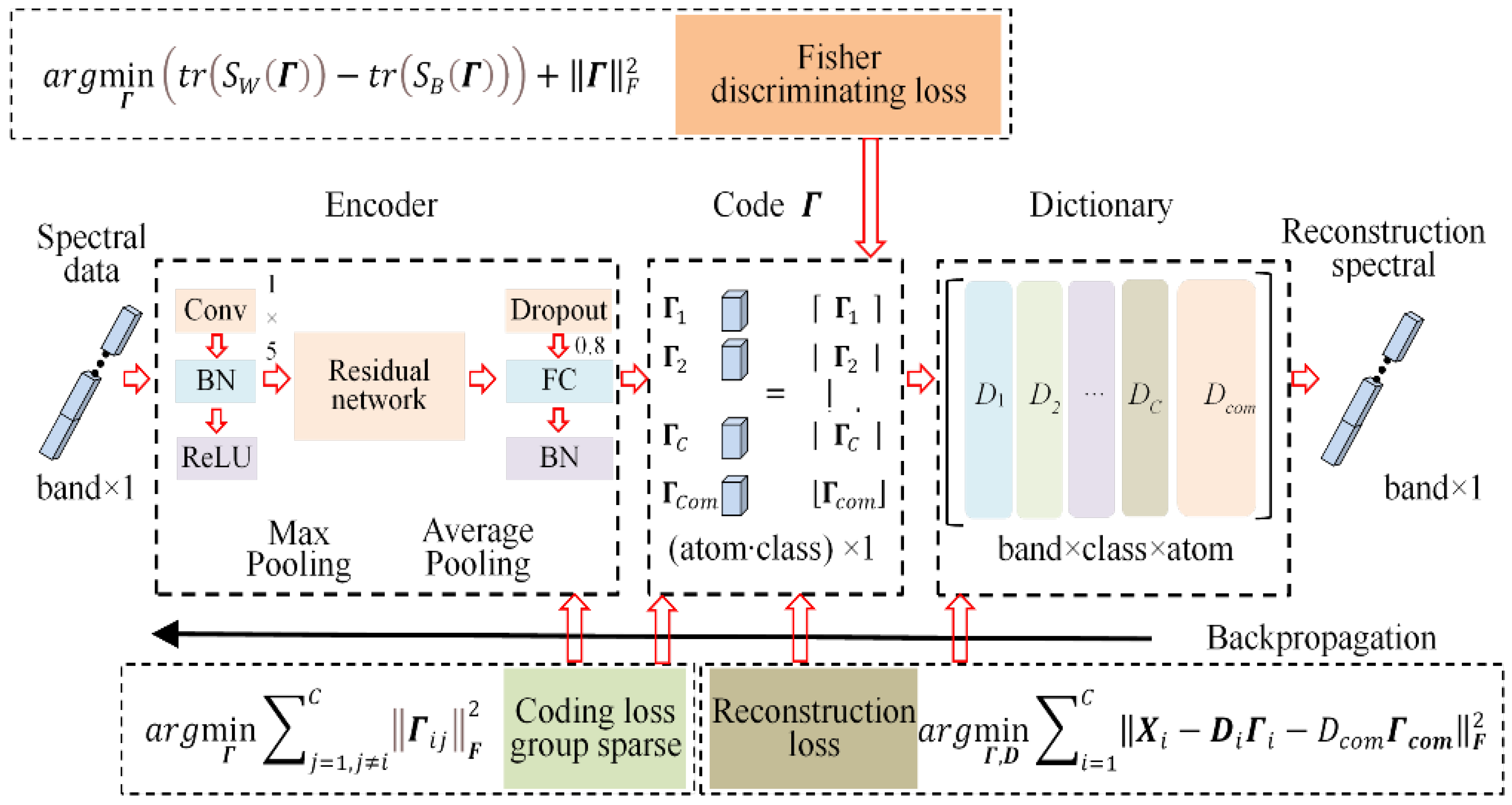
Figure 1 presents the pipeline of the developed framework, with a CNN constructed to encode the spectral information, as well as a structured dictionary established to classify HSIs. Spectral data are first encoded by the CNN model, in which residual networks are used to optimize the main networks. We can acquire the group sparse code using the full connection layer. Meanwhile, two loss functions, i.e., coding loss and Fisher discriminating loss, are calculated to optimize code coefficients. More importantly, a discriminative dictionary is constructed by reconstruction loss to enhance the discriminative ability of the developed model.
2.2.1. Residual Networks Encoder
Compared with the common dictionary-based models using sparse constraints, the group sparsity models have more intensive and effective code coefficients, i.e., the coefficient values converge to the diagonal of the matrix [33] and achieve more effective results in classification applications. Therefore, we replace the sparsity constraint with a group sparsity constraint for the dictionary model and construct an encoder to acquire the group sparsity effect.
Suppose is coding coefficients of discriminative dictionary for spectral samples . We want to construct an encoder , and apply , to project the spectral samples into to a nearly null space, i.e.,
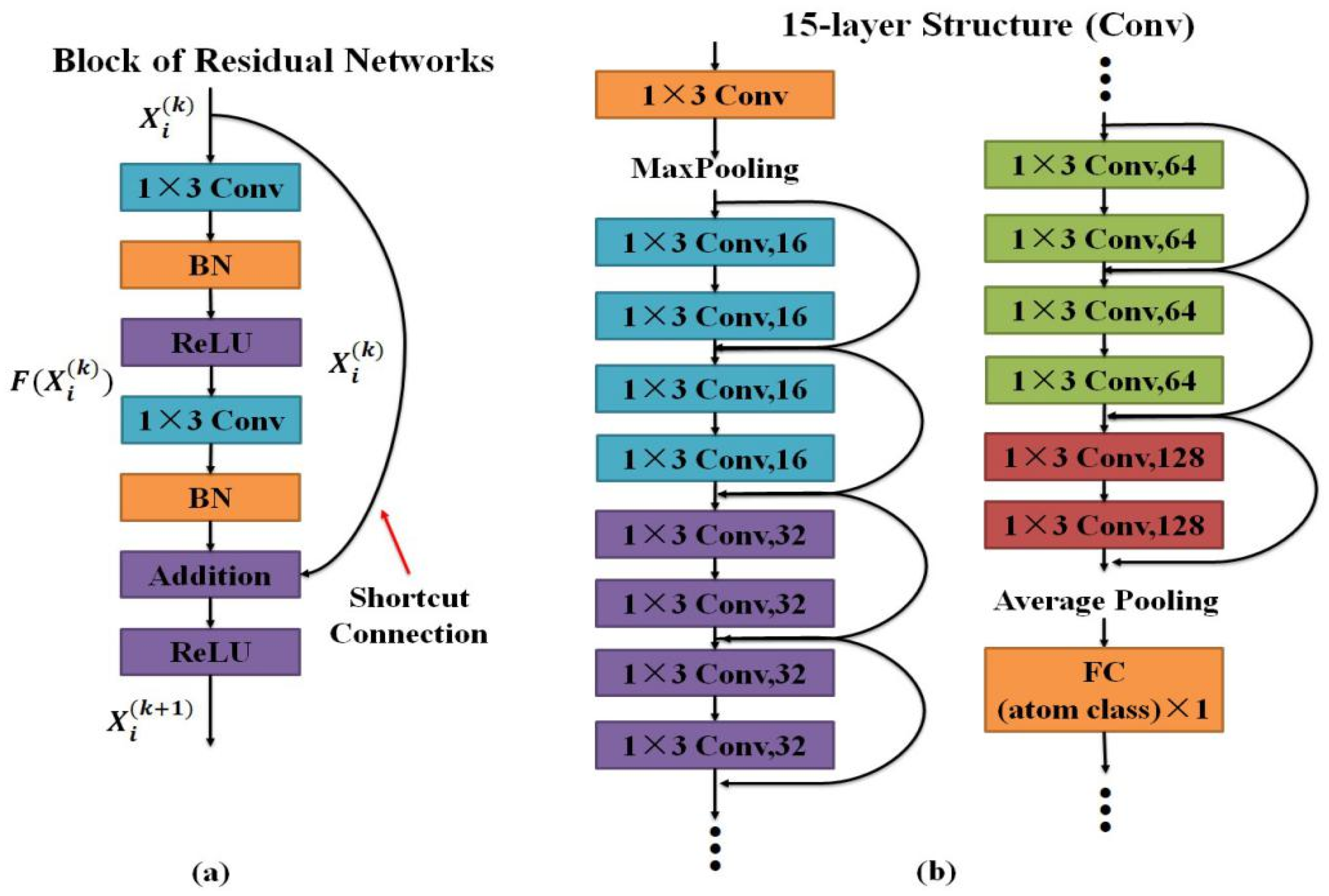
Considering the poor performance of linear projection, a CNN encoder is designed to complete the transformation. Thus, the performance for dictionary learning will be enhanced greatly. He et al. [43] suggested that deeper networks encounter difficulties in the following degradation problem: as the network depth increases, accuracy becomes saturated and then degrades rapidly. Therefore, residual networks are used to address the degradation problem and increase the convergence rate. As depicted in Figure 2, the building block of residual networks (Figure 2a) contains two convolutional layers (Conv), two batch normalization layers (BN), and two leaky ReLU layers. The output of residual networks is calculated as follows:
We explicitly let the stacked nonlinear layers fit the residual function and original mapping is recast into . The formulation of Equation (2) can be realized by feedforward neural networks with “shortcut connections” (Figure 2a). Shortcut connections [43,44] are those skipping one or more layers. The entire network can still be trained end-to-end by stochastic gradient descent (SGD) with backpropagation.
Based on the above block of residual networks, we construct a 15-layer encoder (in terms of convolutional layers) as presented in Figure 2b. We first employ a convolutional layer to capture large receptive field [45] and max pooling is used to select the remarkable values. Then, we design 7 pieces of residual block, in which a convolutional layer is used to acquire effective receptive field. More importantly, feature maps corresponding to various convolutional kernel increase from 16 to 128 to acquire abundant spectral information. Finally, we adopt an average pooling to compress the spectral information and employ a fully connected (FC) layer to connect the coding coefficients. The output number of FC depends on the product of spectral band and sub-dictionary atom numbers. For backpropagation, we use SGD with a batch size of 8. The learning rate starts from 0.1 and epoch number is 500.
We apply the encoder P to extract spectral information from HSI and enforce the code coefficients to be group sparsity. To enhance the discriminative ability of our model, we build a structured dictionary, where each sub-dictionary can be directly used to represent the specific-class samples, i.e., the dictionaries are interpretable. The structure dictionary can be calculated as follows:
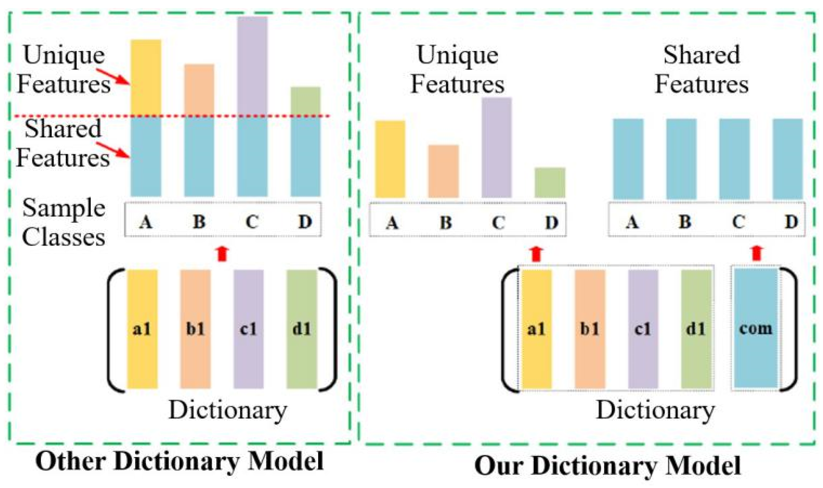
The first term of Equation (3) is the reconstruction loss which is used to construct the structure dictionary. Each sub-dictionary is established and learned from ith class samples. The second term for Equation (3) is the coding loss. However, the structure of existing dictionary needs optimization to learn common and specific features of HSI samples. As depicted in Figure 3, the test samples contain the common characteristics, i.e., the features they shared. To solve this problem, we design the shared constraint for sub-dictionaries. Our shared constraint (the com sub-dictionary) is built to describe duplicated information (common characteristics in Figure 3). Then, the discriminative characteristics will be “amplified” relative to the original characteristics.
2.2.2. Dictionary Learning
Here, we design a sub-dictionary to calculate the class-shared characters as follows:
where denotes the shared (common) sub-dictionary. Each sub-dictionary (both specific and common ones) contains atoms, and each atom is column vector.The matrix of specific and common sub-dictionaries is randomly initialized, and corresponding atoms are constantly updated according to the objective function. The corresponding objective function is modified as follows:
where is the coding coefficient for common sub-dictionary. With the calculation of term , the results of term tend to be closer to zero, and the corresponding reconstructive ability of the structured dictionary will be improved. Meanwhile, the coding loss and discriminating loss will facilitate the construction of shared (common) sub-dictionaries.
In our framework, the dictionary is calculated by the single convolutional layer, and the convolutional weights serve as dictionary coefficients. Therefore, the dictionary is updated by the back-propagation (BP) algorithm. We design additional channels for shared (common) sub-dictionaries that will also be updated during BP processing. The main difference from the CNN model (end-to-end) is that we design a dictionary module, which contains various sub-dictionaries, to optimize the discriminative ability. Moreover, we design coding and discriminating loss for the middle variable (code coefficients ), which is a very different algorithm structure.
2.2.3. Loss Functions
To enhance the discriminative ability of the developed model, we design two kinds of loss functions for the proposed model. First, we design the coding loss to realize a fast and effective spectral data encoding.
Then, Fisher discriminative loss is designed to enhance the discriminative ability of our model. Meanwhile, a reconstruction loss is also used to build the structure dictionary. Overall, we apply three loss functions to optimize the classification performance.
Two kinds of discriminative loss functions can be implemented by programming. One is Fisher discriminative loss and the other is cross-entropy loss . Both loss functions have been implemented in the program, and we will provide two versions of the final program for researchers. In this paper, all of the results are calculated with cross-entropy loss. Figure 4 shows the variation trend of three loss function values and classification accuracy with increasing epoch. All loss functions are convergent, and our approach achieves excellent classification accuracy. Therefore, the final objective function is as follows:
where and are the scalar constants and they will be discussed in experiments.
3. Experimental Results and Analysis
In this section, we quantitatively and qualitatively evaluate the classification performance of the proposed model on four public datasets, namely Pavia [38], Botswana [39], Houston 2013 [40], and Houston 2018 [41]. We compare the performance of the proposed method with other existing algorithms, including SVM [18,21], FDDL [32], DPL [33], ResNet [33], AE [27], RNN [27], CNN [27], and CRNN [27], for HSI classification. We report the overall accuracy (OA), average accuracy (AA) and kappa coefficient [46] of different datasets and present corresponding classification maps. Furthermore, we analyze the classification performance in detail, following each experimental dataset.
3.1. Sample Selection
We randomly choose 10% of the labeled samples in the dataset as the training data. To overcome the imbalance issue, we adopt a weighted sample generation strategy and make all trained samples per class equal to others as follows:
where is the new sample generated by combining of samples and , and is a random constant between 0 and 1. Samples and are randomly selected from the same class of training data. All the methods in comparison are implemented on the balanced dataset in this strategy.
3.2. Parameter Setting
In the proposed model, two groups of free parameters need to be adjusted: (1) the number of dictionary atoms and (2) regularization parameters and . The above parameter settings are a critical factor to ensure the performance of the model and will be analyzed.
3.2.1. Number of Dictionary Atoms
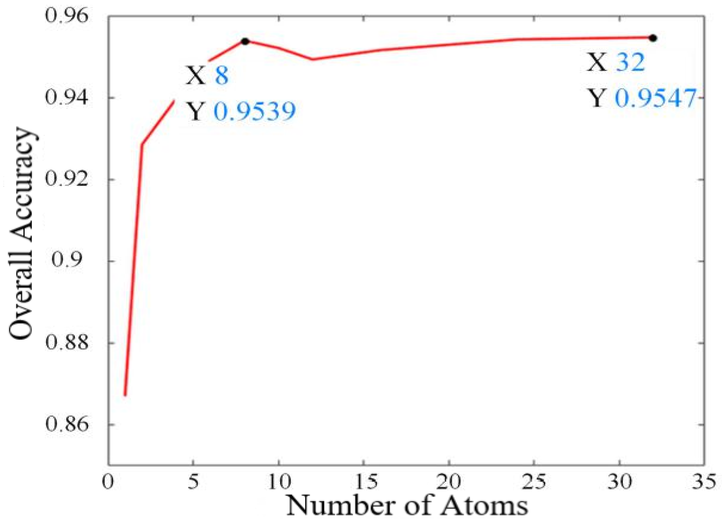
We set all the subdictionaries to have the same number atoms. The number of atoms is adaptively estimated with Houston 2013 datasets, as depicted in Figure 5. The classification OA increases with the number of atoms for each sub-dictionary (atom number under 8), while the changes in OA are not enormous along with the variation in atom number beyond 10. We set the number of atoms to 8 for each dataset to efficiently train the developed model.
3.2.2. Constraint Coefficients and
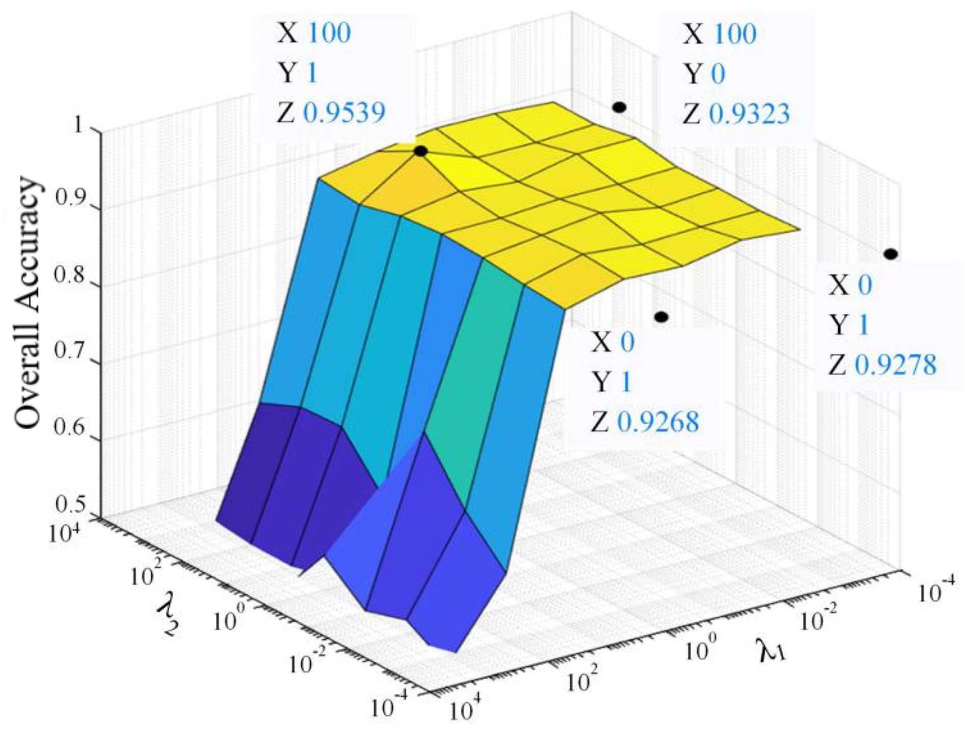
and mainly balance reconstruction and coding loss in Equation (6). We test the proposed model with regularization parameters and ranging from 0 to , and select the value of parameter with the highest accuracy. Figure 6 presents the visualized result on Houston 2013 datasets. The OA values will decrease greatly with the increasing of (beyond 10). This result demonstrates that our model is sensitive for coding loss. We set and for the classification of Houston 2013 dataset.
3.3. Classification Performance Analysis for Different Datasets
3.3.1. Center of Pavia
Table 1 shows the classification results of the compared algorithms. According to the presented score, our method outperforms other algorithms, especially on Water, Tiles, and Bare Soil surface regions. Benefiting from the designed deep and sub-dictionary framework, the proposed method is more outstanding than other dictionary learning-based method (i.e., FDDL). Compared with other CNN-based models, by involving dictionary structure, our method shows better deep feature extraction ability and achieves higher OA, AA, and kappa coefficients with , and , respectively. In addition, Figure 7 presents the confusion matrix of the developed model, which also indicates an effective discrimination ability for surface regions.
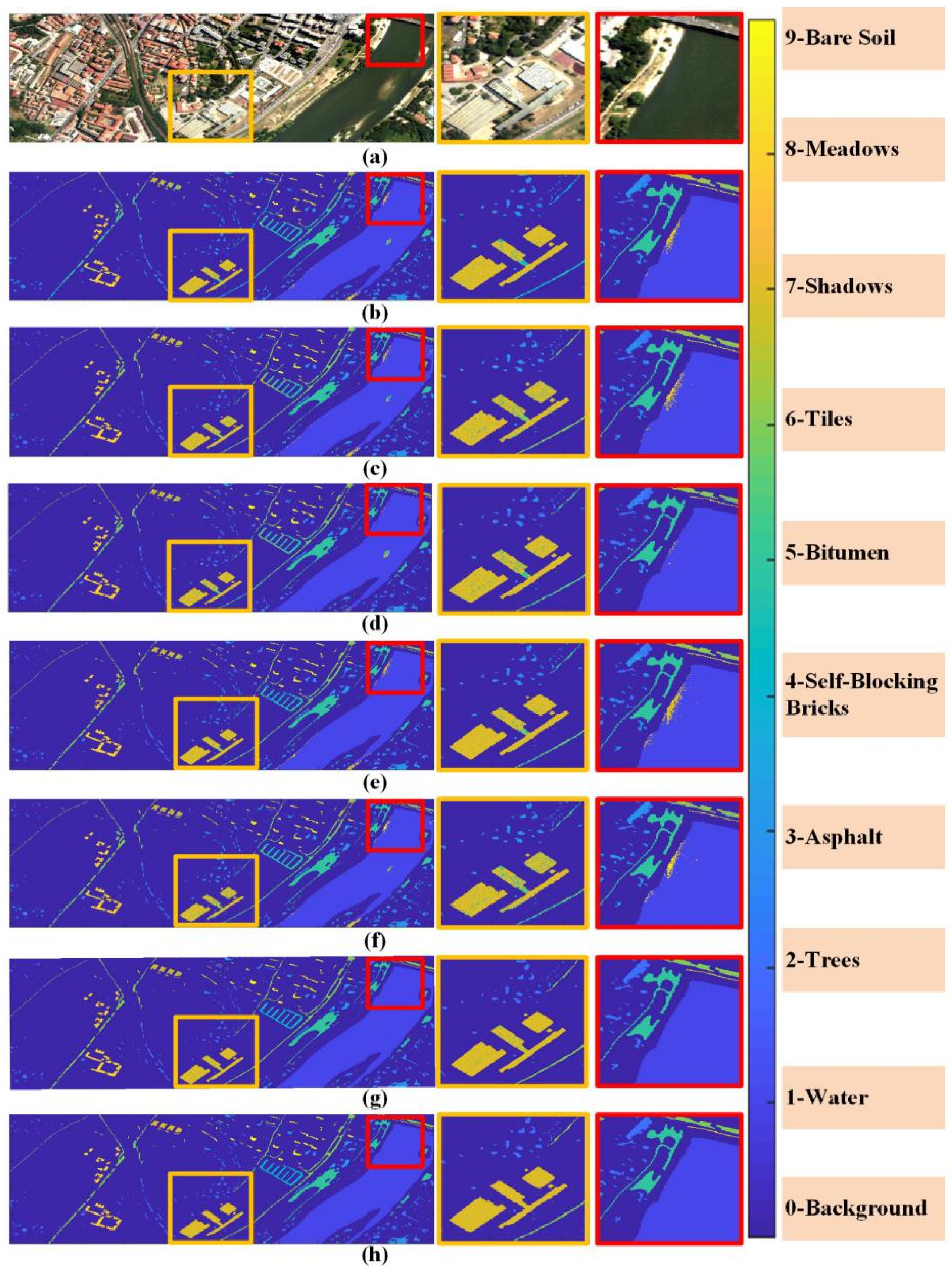
Figure 8 presents the classification maps acquired by various methods on the Center of Pavia data set. Figure 8a,h are the pseudo-color image and ground truth map, and Figure 8b–g depicts the corresponding classification maps of FDDL, DPL, ResNet, RNN, CNN, and the proposed model, respectively. It can be seen that our method shows better visual performance than the dictionary and CNN-based algorithms in both the smoothness in same material region and sharpness on the edges between different material one. For better comparison, we highlight river bank and building regions with red and yellow rectangles in Figure 8. In terms of the classification results in the red rectangle, all of the methods, except the CNN model and our method, incorrectly classify some water samples into Bare Soil class. As for the yellow rectangle region, our model achieved smoothest classification results on Bara Soil class in which CNN method confuses some samples into Bitumen class, which leads to a inferior score when comparing with our proposed algorithm.
3.3.2. Botswana
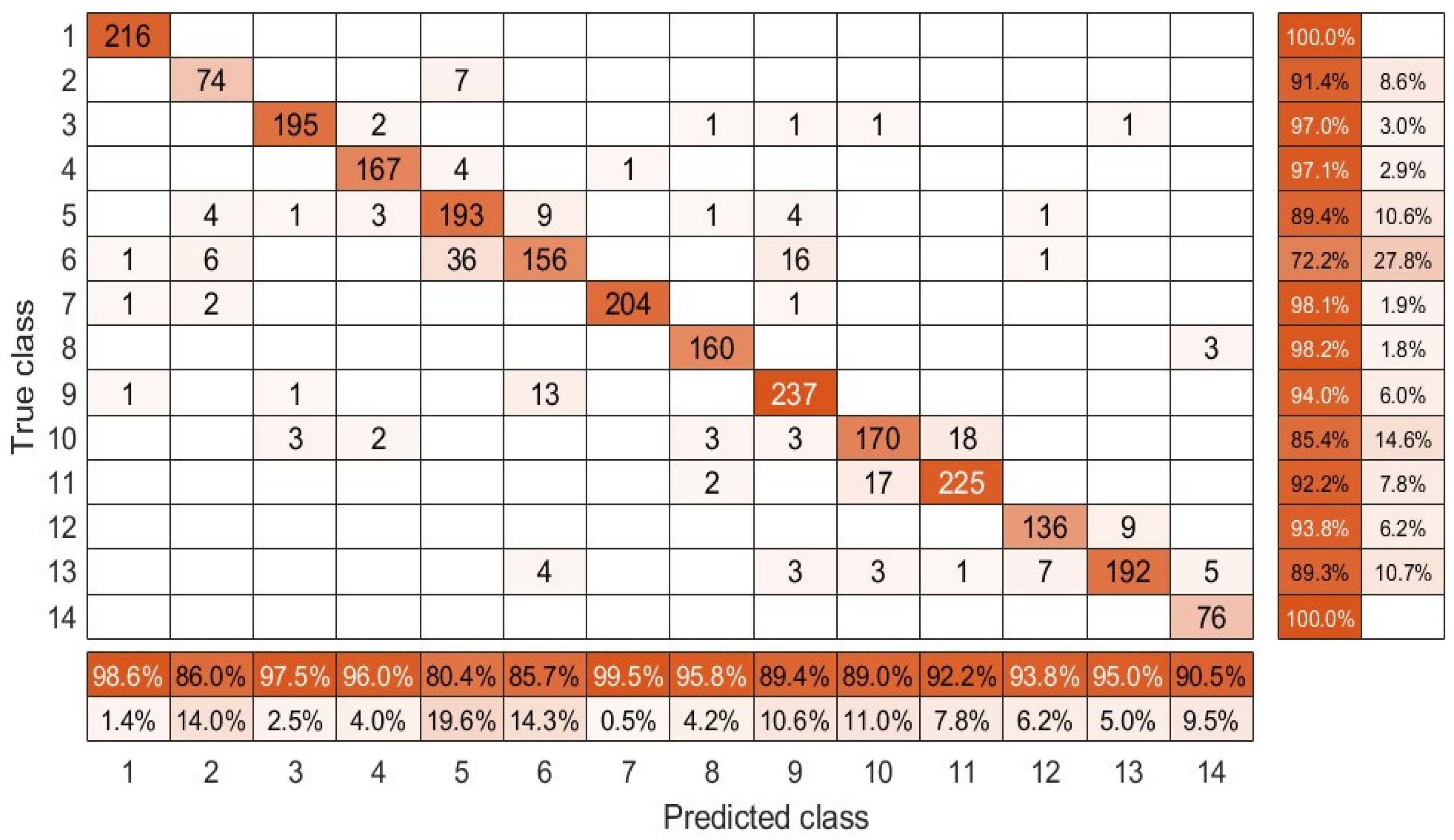
Table 2 presents the class-specific classification accuracy in terms of the Botswana data set, where our algorithm achieves the highest classification accuracy in over 50 percent of the classes (8 out of total 14 classes). In particular, our method performs better than other comparison methods in classes Reeds, Acacia Woodlands, and Exposed Soils. To be more specific, for the Reeds class our method is almost higher than the others, and higher than comparison methods for the Exposed Soils class. In addition, according to the corresponding confusion matrix in Figure 9, our algorithm outperforms other methods in terms of OA, AA, and kappa coefficients with , , and , respectively. Such performance could further demonstrate the superior discrimination classification capability for our model.
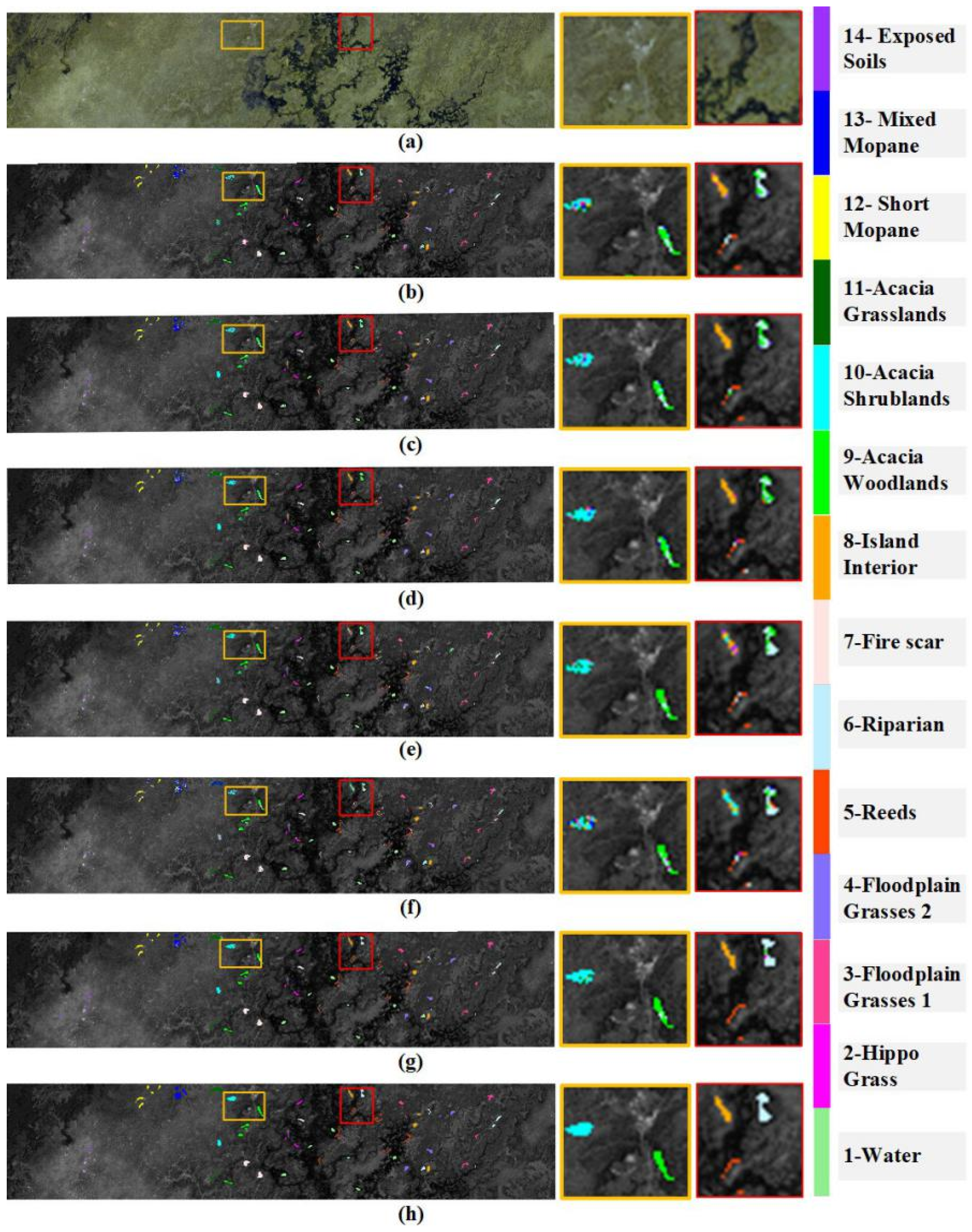
Figure 10 shows the classification maps for the Botswana dataset, where Figure 10a,h are the pseudo-color image and ground truth map, and Figure 10b–g are the corresponding classification results of FDDL, DPL, ResNet, RNN, CNN, and the proposed model. We mark the most misplaced regions with yellow and red rectangles for more obvious comparison. As shown in yellow rectangle region, Acacia Woodlands and Acacia Shrublands are wrongly classified into Exposed Soils or the Floodplain Grasses 1 class by other methods. As for the rectangles colored red, other methods almost lose the ability to distinguish between different land covers, i.e., the CNN method misclassified the Island Interior class into the Acacia Shrublands class. In contrast, our approach removed noisy scattered points and led to smoother classification results without blurring the boundaries. The superior performance could be owing to the effectiveness of the proposed structured dictionary learning model.
3.3.3. Houston 2013
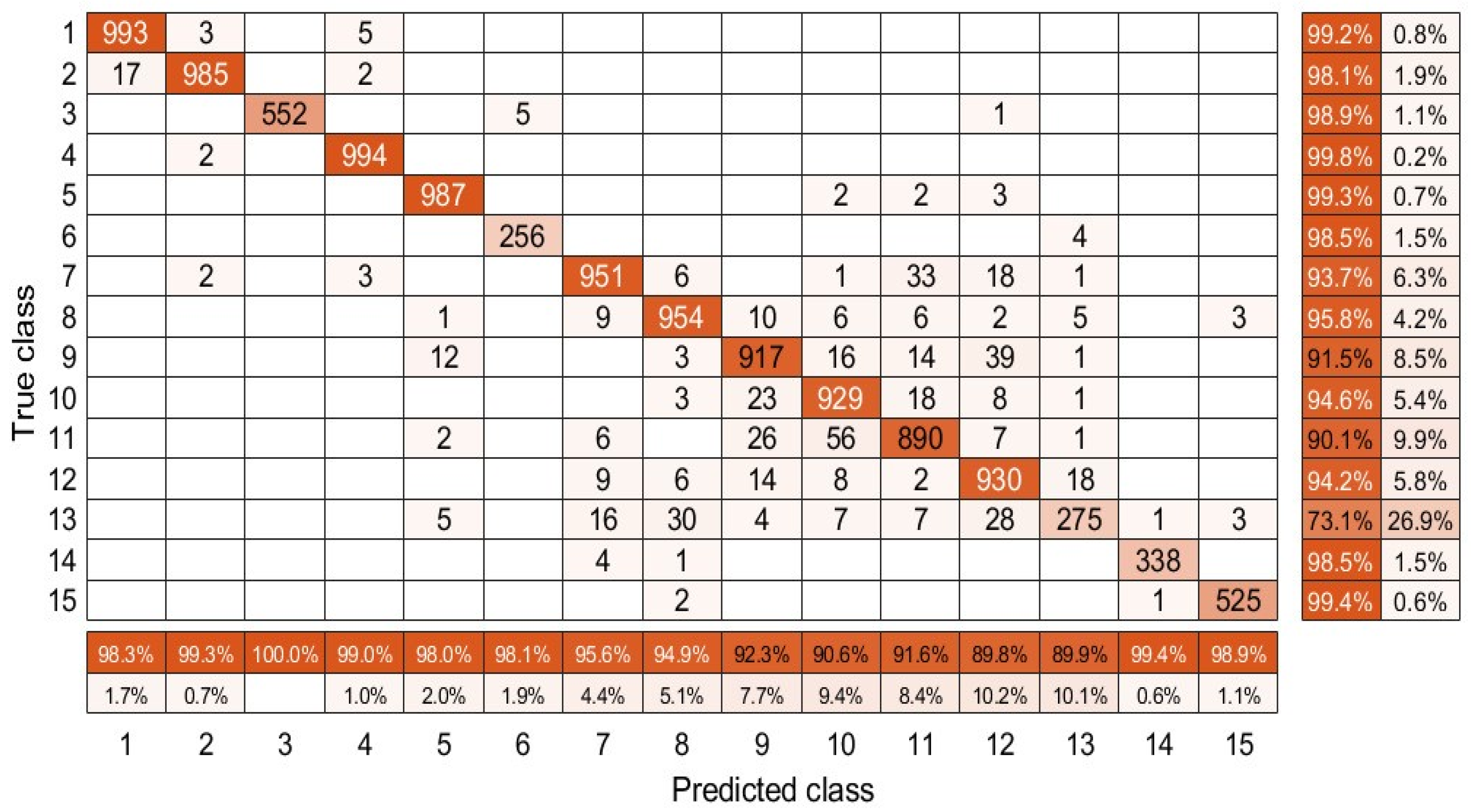
The classification results achieved by the methods in comparison on the Houston 2013 dataset are presented in Table 3, and Figure 11 presents the confusion matrix relative to the developed model. As depicted in Table 3, the classification results is more than higher than other methods on classes Commercial, Road, Highway and Parking Lot 1, while it performs competitively with other methods for other classes. Specifically, for Stressed Grass class, our method only is lower than AE method and lower than CNN method, but almost two percent in average higher than the other methods. It is noteworthy that the developed algorithm outperforms other operators in feature extraction generally for OA, AA and kappa with , , and , respectively. Furthermore, the confusion matrix in Figure 11 also reveals that the algorithm here can be effective to distinguish a surface region.
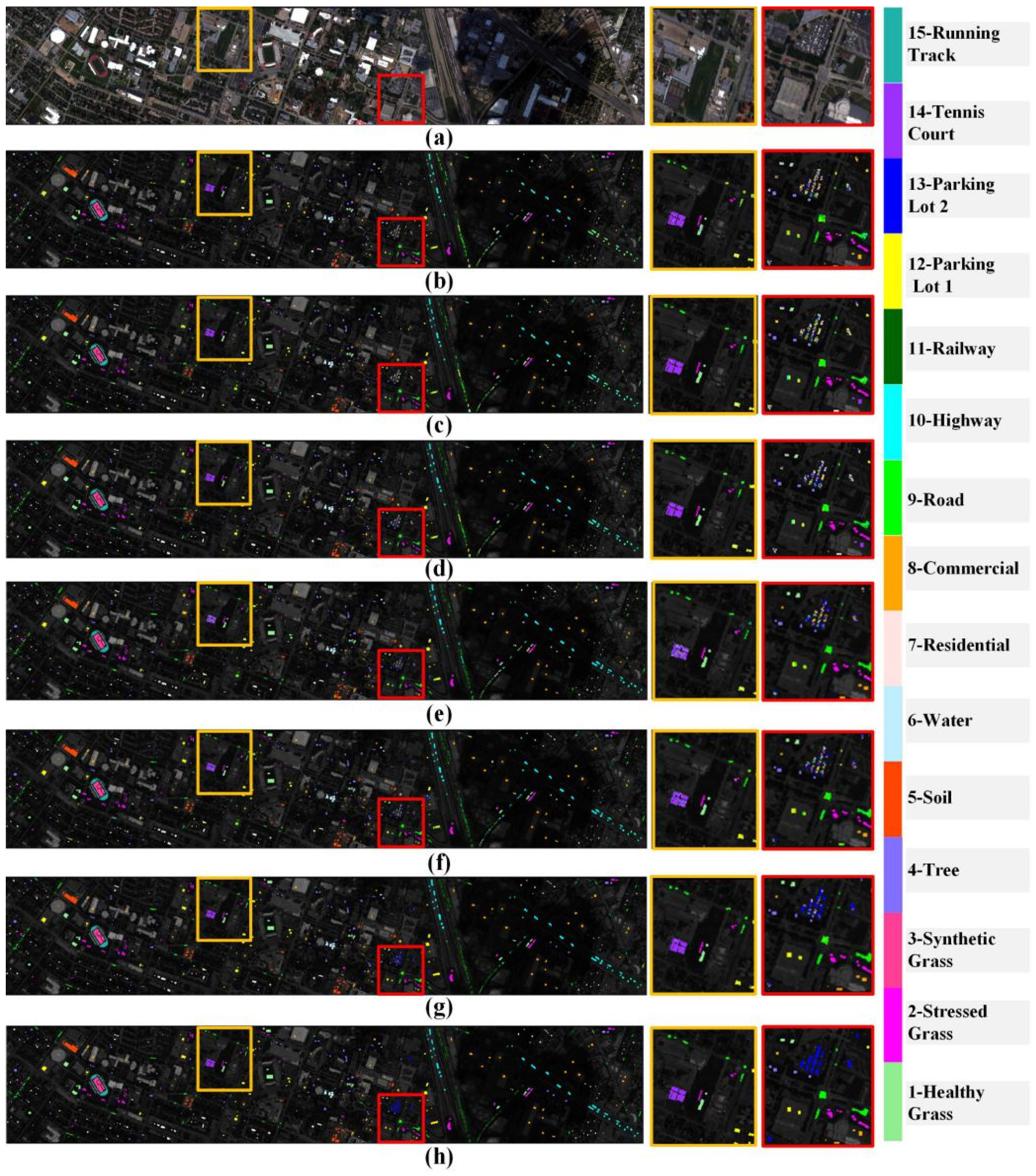
Figure 12 depicts the classification map generated by the approaches in comparison on Houston 2013 dataset. Figure 12a,h shows the pseudo-color image and ground truth map, and Figure 12b–g shows the corresponding classification results thereof. We label the misclassified regions which contain buildings and cars with yellow and red rectangles, respectively. According to the ground truth in yellow regions, there exists a small Parking Lot 1 class but this is misplaced by most of the methods. Specifically, the classification of DPL, RNN, and CNN contain many misclassified points which lead to an unsatisfactory classification effect. For the red one, the other algorithms show significant misclassification of the Parking Lot 2 class, FDDL, DPL and ResNet are unable to distinguish between Parking Lot 2 and Parking Lot 1 classes. In contrast, as impacted by the robust property within the spectra’s local variation, our method showed more complete and correct classification results. Besides that, our method also achieved an effective removal of salt-and-pepper noise effects from the classification map. Moreover, it maintains the significant objects or structures. The developed model acquires a classification map with higher accuracy around and in the parking lot due to the robust property in the spectra’s local variation.
3.3.4. Houston 2018
Table 4 and Figure 13 present the classification results and confusion matrix on Houston 2018 datasets in comparison with other algorithms, respectively. According to the results, one can see that the classification accuracy decreases for each method when compared to the one in the Houston 2013 dataset. This phenomenon is more obvious for sidewalk and crosswalk classes, where the highest scores are only and , respectively. We believe that the decrease could be attributed to the increase of land cover types and the reduction of spectral information (only 46 spectral bands). In addition, our method ranks first in 9 out of 20 total classes of land covers and our method also outperforms other algorithms at least two points in terms of OA, AA, and kappa indicators. Furthermore, our model also shows significant discriminative ability between 20 classes according to the confusion matrix as illustrated in Figure 13.
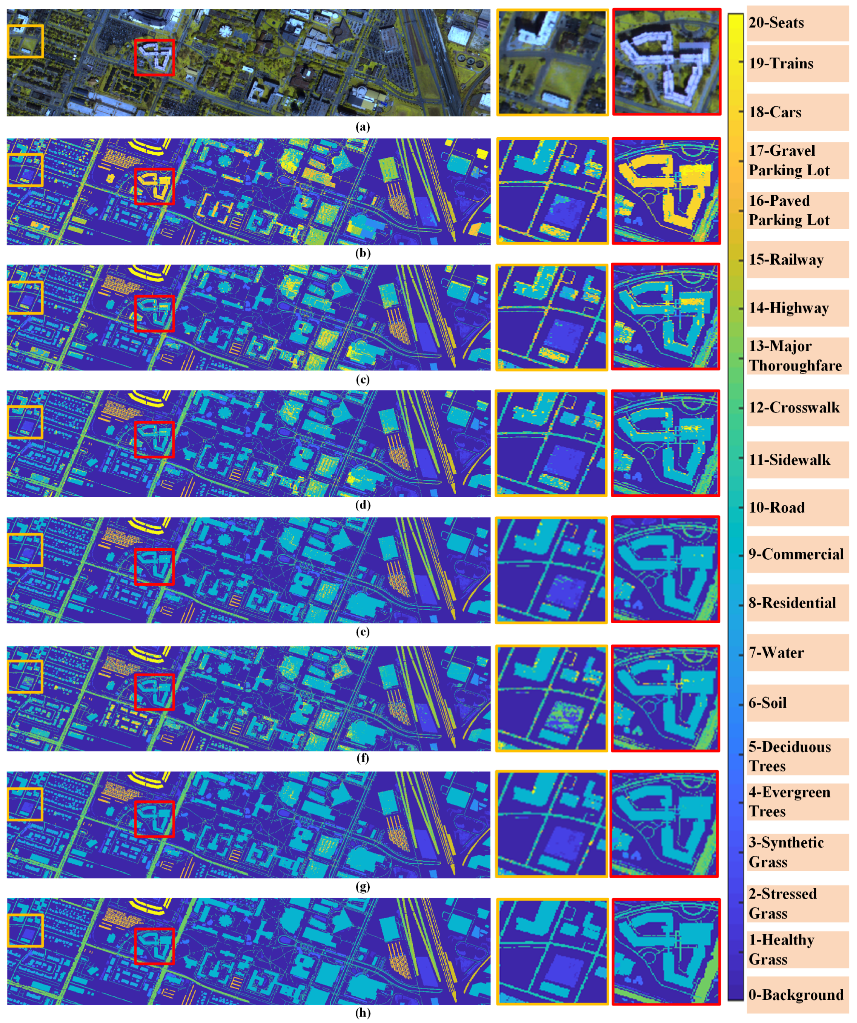
Figure 14 highlights the superiority of the proposed method by means of classification maps on Houston 2018 dataset. Figure 14a,h shows the pseudo-color image and ground truth map, and Figure 14b–g shows the corresponding classification results of FDDL, DPL, ResNet, RNN, CNN, and the proposed model. For better visualization, we marked the Commercial, Road, Major Thoroughfares, and Stressed grass with yellow and red rectangles. According to the yellow rectangles, FDDL and DPL classify the Commercial into the Seats class, and they fail to identify the Road class owing to their poor ability to extract deeper spectral information. For the region of the red rectangle, RNN and CNN misclassified small Road into Cars. Moreover, there also exist some noisy points in the Commercial class. In contrast, our models showed more smooth and complete classification results.
According to the experimental results above, our approach achieved the highest OA, AA, and kappa coefficient on four benchmark datasets which were collected by different sensors with various land covers. Compared with other dictionary-based and CNN-based models, our model generally achieves smoother and more accurate classification results, especially for the large area of homogeneous land cover and the irregular small area types. The aforementioned experiments verified that benefiting from the rationally designed structure classification layer (dictionary) and loss functions, our model has the capability to extract the intrinsic invariant spectral feature representation from the HSI and achieves more effective feature extraction.
4. Discussion
In the last section, we presented the result and analysis of experiments on each dataset. In this section, we analyze and discuss the key factors, which affect the performance of the algorithm and need to be considered in practical HSI classification applications.
4.1. Influence of Imbalanced Samples
Chang et al. [47] suggested that imbalanced data will be of great significance to the HSI classification. To explore the effect arising from imbalanced data on classification performance, we randomly choose 10% of the labeled sample of each class and performed an experiment on Houston 2013 dataset with imbalanced data, as listed in Table 5. The imbalanced data will reduce the classification performance, leading to a decrease of about 3∼4% in classification accuracy. Our model still achieves the best performance when the training data are imbalanced. The classification results confirm the powerful classification ability of our model.
4.2. Influence of Small Training Samples
To confirm the effectiveness of our framework in practical scenario with the absence of samples, we reduce the number of training samples into 10, 20, and 30 per class. As listed in Table 6, we observed that the models generally suffer from unstable classification performance for different classes. Overall, the proposed model can achieve the best results in most of the indices with an increase of at least 4% accuracy compared with CNN-based models. We will obtain a better classification result with the increasing training data which corresponds with the results.
4.3. Computational Cost
Another factor that affects the practical application of the HSI classification model is the efficiency of the algorithm. Therefore, we present the computational time-consuming for the comparison algorithms.
All the tests here are performed on an Intel Core i7-8700 CPU 3.20 GHz desktop with 16 GB memory and carried out by employing Python on the Windows 10 operating system. In Table 7, we can see that the developed model has a slower running speed than DPL, which applies linear projection to extract spectral features. However, the developed model achieves faster testing speed than CNN-based models due to its simpler convolutional structure.
5. Conclusions
In this paper, we propose a novel deep learning-based structure dictionary model to extract spectral features from HSIs. Specifically, a residual network is used with a dictionary learning framework to strengthen the feature representation for the original data. Afterwards, sub-dictionaries with shared constraints are introduced to extract the common feature for samples with different class label. Moreover, three kinds of loss functions are combined to enhance the discriminative ability for the overall model. Numerous tests were carried out on HSI datasets, and qualitatively and quantitatively results showed that the proposed feature learning model requires much less computation time when comparing with other SVM and CNN-based models, demonstrating its potential and superiority in HSI classification tasks.
Author Contributions
Funding acquisition, Y.H. and C.D.; Methodology, W.W. and Z.L.; Supervision, C.D.; Validation, Z.L.; Writing original draft, W.W. and Y.H. All authors have read and agreed to the published version of this manuscript.
Funding
This study receives support from China Postdoctoral Science Foundation under Grant 2021TQ0177 and the National Natural Science Foundation of China (NSFC) under Grant 62171040.
Data Availability Statement
Conflicts of Interest
The authors declare no conflict of interest.
References
- Ghamisi, P.; Plaza, J.; Chen, Y.; Li, J.; Plaza, A.J. Advanced spectral classifiers for hyperspectral images: A review. IEEE Geosci. Remote Sens. Mag. 2017, 5, 8–32. [Google Scholar] [CrossRef] [Green Version]
- Hong, D.; Yokoya, N.; Chanussot, J.; Zhu, X.X. An augmented linear mixing model to address spectral variability for hyperspectral unmixing. IEEE Trans. Image Process. 2018, 28, 1923–1938. [Google Scholar] [CrossRef] [PubMed] [Green Version]
- Li, J.; Huang, X.; Gamba, P.; Bioucas-Dias, J.M.; Zhang, L.; Benediktsson, J.A.; Plaza, A. Multiple feature learning for hyperspectral image classification. IEEE Trans. Geosci. Remote Sens. 2014, 53, 1592–1606. [Google Scholar] [CrossRef] [Green Version]
- Hong, D.; Gao, L.; Yokoya, N.; Yao, J.; Chanussot, J.; Du, Q.; Zhang, B. More diverse means better: Multimodal deep learning meets remote-sensing imagery classification. IEEE Trans. Geosci. Remote Sens. 2020, 59, 4340–4354. [Google Scholar] [CrossRef]
- Hong, D.; Gao, L.; Yokoya, N.; Yao, J.; Chanussot, J.; Du, Q.; Zhang, B. Joint and progressive subspace analysis (JPSA) with spatial-spectral manifold alignment for semi-supervised hyperspectral dimensionality reduction. IEEE Trans. Cybern. 2021, 51, 3602–3615. [Google Scholar] [CrossRef]
- Hong, D.; Gao, L.; Yao, J.; Zhang, B.; Plaza, A.; Chanussot, J. Graph convolutional networks for hyperspectral image classification. IEEE Trans. Geosci. Remote Sens. 2020, 59, 5966–5978. [Google Scholar] [CrossRef]
- Hong, D.; Gao, L.; Yao, J.; Yokoya, N.; Chanussot, J.; Heiden, U.; Zhang, B. Endmember-guided unmixing network (EGU-Net): A general deep learning framework for self-supervised hyperspectral unmixing. IEEE Trans. Neural Netw. Learn. Syst. 2021. [Google Scholar] [CrossRef]
- Liu, X.; Deng, C.; Chanussot, J.; Hong, D.; Zhao, B. StfNet: A two-stream convolutional neural network for spatiotemporal image fusion. IEEE Trans. Geosci. Remote Sens. 2019, 57, 6552–6564. [Google Scholar] [CrossRef]
- Kumar, S.; Ghosh, J.; Crawford, M.M. Best-bases feature extraction algorithms for classification of hyperspectral data. IEEE Trans. Geosci. Remote Sens. 2001, 39, 1368–1379. [Google Scholar] [CrossRef] [Green Version]
- Rashwan, S.; Dobigeon, N. A split-and-merge approach for hyperspectral band selection. IEEE Geosci. Remote Sens. Lett. 2017, 14, 1378–1382. [Google Scholar] [CrossRef] [Green Version]
- Jolliffe, I.T. Principal component analysis. Technometrics 2003, 45, 276. [Google Scholar]
- Senthilnath, J.; Omkar, S.; Mani, V.; Karnwal, N.; Shreyas, P. Crop stage classification of hyperspectral data using unsupervised techniques. IEEE J. Sel. Top. Appl. Earth Obs. Remote Sens. 2012, 6, 861–866. [Google Scholar] [CrossRef]
- Green, A.A.; Berman, M.; Switzer, P.; Craig, M.D. A transformation for ordering multispectral data in terms of image quality with implications for noise removal. IEEE Trans. Geosci. Remote Sens. 1988, 26, 65–74. [Google Scholar] [CrossRef] [Green Version]
- Schölkopf, B.; Smola, A.; Müller, K.R. Nonlinear component analysis as a kernel eigenvalue problem. Neural Comput. 1998, 10, 1299–1319. [Google Scholar] [CrossRef] [Green Version]
- Mei, F.; Zhao, C.; Wang, L.; Huo, H. Anomaly detection in hyperspectral imagery based on kernel ICA feature extraction. In Proceedings of the 2008 Second International Symposium on Intelligent Information Technology Application, Shanghai, China, 20–22 December 2008; Volume 1, pp. 869–873. [Google Scholar]
- Fauvel, M.; Chanussot, J.; Benediktsson, J.A. Kernel principal component analysis for the classification of hyperspectral remote sensing data over urban areas. EURASIP J. Adv. Signal Process. 2009, 2009, 1–14. [Google Scholar] [CrossRef] [Green Version]
- Marchesi, S.; Bruzzone, L. ICA and kernel ICA for change detection in multispectral remote sensing images. In Proceedings of the 2009 IEEE International Geoscience and Remote Sensing Symposium, Cape Town, South Africa, 12–17 July 2009; Volume 2. [Google Scholar]
- Cortes, C.; Vapnik, V. Support vector networks. Mach. Learn. 1995, 20, 273–297. [Google Scholar] [CrossRef]
- Camps-Valls, G.; Bruzzone, L. Kernel-based methods for hyperspectral image classification. IEEE Trans. Geosci. Remote Sens. 2005, 43, 1351–1362. [Google Scholar] [CrossRef]
- Bruzzone, L.; Chi, M.; Marconcini, M. A novel transductive SVM for semisupervised classification of remote-sensing images. IEEE Trans. Geosci. Remote Sens. 2006, 44, 3363–3373. [Google Scholar] [CrossRef] [Green Version]
- Zhao, C.; Liu, W.; Xu, Y.; Wen, J. A spectral-spatial SVM-based multi-layer learning algorithm for hyperspectral image classification. Remote Sens. Lett. 2018, 9, 218–227. [Google Scholar] [CrossRef]
- Li, S.; Song, W.; Fang, L.; Chen, Y.; Ghamisi, P.; Benediktsson, J.A. Deep learning for hyperspectral image classification: An overview. IEEE Trans. Geosci. Remote Sens. 2019, 57, 6690–6709. [Google Scholar] [CrossRef] [Green Version]
- Chen, Y.; Lin, Z.; Zhao, X.; Wang, G.; Gu, Y. Deep learning-based classification of hyperspectral data. IEEE J. Sel. Top. Appl. Earth Obs. Remote Sens. 2014, 7, 2094–2107. [Google Scholar] [CrossRef]
- Chen, Y.; Zhao, X.; Jia, X. Spectral–spatial classification of hyperspectral data based on deep belief network. IEEE J. Sel. Top. Appl. Earth Obs. Remote Sens. 2015, 8, 2381–2392. [Google Scholar] [CrossRef]
- Shi, C.; Pun, C.M. Multi-scale hierarchical recurrent neural networks for hyperspectral image classification. Neurocomputing 2018, 294, 82–93. [Google Scholar] [CrossRef]
- Hang, R.; Liu, Q.; Hong, D.; Ghamisi, P. Cascaded recurrent neural networks for hyperspectral image classification. IEEE Trans. Geosci. Remote Sens. 2019, 57, 5384–5394. [Google Scholar] [CrossRef] [Green Version]
- Rasti, B.; Hong, D.; Hang, R.; Ghamisi, P.; Kang, X.; Chanussot, J.; Benediktsson, J.A. Feature extraction for hyperspectral imagery: The evolution from shallow to deep: Overview and toolbox. IEEE Geosci. Remote Sens. Mag. 2020, 8, 60–88. [Google Scholar] [CrossRef]
- Wright, J.; Yang, A.Y.; Ganesh, A.; Sastry, S.S.; Ma, Y. Robust face recognition via sparse representation. IEEE Trans. Pattern Anal. Mach. Intell. 2008, 31, 210–227. [Google Scholar] [CrossRef] [Green Version]
- Chen, Y.; Nasrabadi, N.M.; Tran, T.D. Hyperspectral image classification using dictionary-based sparse representation. IEEE Trans. Geosci. Remote Sens. 2011, 49, 3973–3985. [Google Scholar] [CrossRef]
- Gao, L.; Yu, H.; Zhang, B.; Li, Q. Locality-preserving sparse representation-based classification in hyperspectral imagery. J. Appl. Remote Sens. 2016, 10, 042004. [Google Scholar] [CrossRef]
- Yang, M.; Zhang, L.; Yang, J.; Zhang, D. Metaface learning for sparse representation based face recognition. In Proceedings of the 2010 IEEE International Conference on Image Processing, Hong Kong, China, 26–29 September 2010; pp. 1601–1604. [Google Scholar]
- Yang, M.; Zhang, L.; Feng, X.; Zhang, D. Fisher discrimination dictionary learning for sparse representation. In Proceedings of the 2011 International Conference on Computer Vision, Barcelona, Spain, 6–13 November 2011; pp. 543–550. [Google Scholar]
- Gu, S.; Zhang, L.; Zuo, W.; Feng, X. Projective dictionary pair learning for pattern classification. Adv. Neural Inf. Process. Syst. 2014, 27. [Google Scholar]
- Akhtar, N.; Mian, A. Nonparametric coupled Bayesian dictionary and classifier learning for hyperspectral classification. IEEE Trans. Neural Netw. Learn. Syst. 2017, 29, 4038–4050. [Google Scholar] [CrossRef]
- Tu, X.; Shen, X.; Fu, P.; Wang, T.; Sun, Q.; Ji, Z. Discriminant sub-dictionary learning with adaptive multiscale superpixel representation for hyperspectral image classification. Neurocomputing 2020, 409, 131–145. [Google Scholar] [CrossRef]
- Tang, H.; Liu, H.; Xiao, W.; Sebe, N. When dictionary learning meets deep learning: Deep dictionary learning and coding network for image recognition with limited data. IEEE Trans. Neural Netw. Learn. Syst. 2020, 32, 2129–2141. [Google Scholar] [CrossRef] [PubMed]
- Tao, L.; Zhou, Y.; Jiang, X.; Liu, X.; Zhou, Z. Convolutional neural network-based dictionary learning for SAR target recognition. IEEE Geosci. Remote Sens. Lett. 2020, 18, 1776–1780. [Google Scholar] [CrossRef]
- Liu, Q.; Zhou, F.; Hang, R.; Yuan, X. Bidirectional-convolutional LSTM based spectral-spatial feature learning for hyperspectral image classification. Remote Sens. 2017, 9, 1330. [Google Scholar] [CrossRef] [Green Version]
- Yang, H.L.; Crawford, M.M. Spectral and spatial proximity-based manifold alignment for multitemporal hyperspectral image classification. IEEE Trans. Geosci. Remote Sens. 2016, 54, 51–64. [Google Scholar] [CrossRef]
- Debes, C.; Merentitis, A.; Heremans, R.; Hahn, J.; Frangiadakis, N.; Kasteren, T.; Liao, W.; Bellens, R.; Pižurica, A.; Gautama, S. Hyperspectral and LiDAR Data Fusion: Outcome of the 2013 GRSS Data Fusion Contest. IEEE J. Sel. Top. Appl. Earth Obs. Remote Sens. 2014, 7, 2405–2418. [Google Scholar] [CrossRef]
- Xu, Y.; Du, B.; Zhang, L.; Cerra, D.; Pato, M.; Carmona, E.; Prasad, S.; Yokoya, N.; Hänsch, R.; Le Saux, B. Advanced Multi-Sensor Optical Remote Sensing for Urban Land Use and Land Cover Classification: Outcome of the 2018 IEEE GRSS Data Fusion Contest. IEEE J. Sel. Top. Appl. Earth Obs. Remote Sens. 2019, 12, 1709–1724. [Google Scholar] [CrossRef]
- Kong, S.; Wang, D. A brief summary of dictionary learning based approach for classification (revised). arXiv 2012, arXiv:1205.6544. [Google Scholar]
- He, K.; Zhang, X.; Ren, S.; Sun, J. Deep residual learning for image recognition. In Proceedings of the IEEE Conference on Computer Vision and Pattern Recognition, Las Vegas, NV, USA, 27–30 June 2016; pp. 770–778. [Google Scholar]
- Sandler, M.; Howard, A.; Zhu, M.; Zhmoginov, A.; Chen, L.C. Mobilenetv2: Inverted residuals and linear bottlenecks. In Proceedings of the IEEE Conference on Computer Vision and Pattern Recognition, Salt Lake City, UT, USA, 18–23 June 2018; pp. 4510–4520. [Google Scholar]
- Luo, W.; Li, Y.; Urtasun, R.; Zemel, R. Understanding the effective receptive field in deep convolutional neural networks. In Proceedings of the 30th International Conference on Neural Information Processing Systems, Barcelona, Spain, 5–10 December 2016; Volume 29. [Google Scholar]
- Sinha, B.; Yimprayoon, P.; Tiensuwan, M. Cohen’s Kappa Statistic: A Critical Appraisal and Some Modifications. Math. Calcutta Stat. Assoc. Bull. 2006, 58, 151–170. [Google Scholar] [CrossRef]
- Chang, C.I.; Ma, K.Y.; Liang, C.C.; Kuo, Y.M.; Chen, S.; Zhong, S. Iterative random training sampling spectral spatial classification for hyperspectral images. IEEE J. Sel. Top. Appl. Earth Obs. Remote Sens. 2020, 13, 3986–4007. [Google Scholar] [CrossRef]
Figure 1.
Workflow of the proposed feature extraction model.

Figure 2.
Network architectures for our encoder: (a) a block of residual networks, (b) main structure of CNNs.
Figure 2.
Network architectures for our encoder: (a) a block of residual networks, (b) main structure of CNNs.

Figure 3.
Overview of the built dictionary of the developed model. Shared constraints are used to describe the common features of all classes of HSI samples.
Figure 3.
Overview of the built dictionary of the developed model. Shared constraints are used to describe the common features of all classes of HSI samples.

Figure 4.
The loss function value of training samples and classification accuracy of the developed model versus the number of epochs.
Figure 4.
The loss function value of training samples and classification accuracy of the developed model versus the number of epochs.

Figure 5.
The classification OA under different numbers of atoms for each sub-dictionary.

Figure 6.
The classification OA under different regularization parameters and .

Figure 7.
The confusion matrix of the developed model on the Center of Pavia dataset.

Figure 8.
Classification maps of the Center of Pavia dataset with methods in comparison: (a) pseudo-color image; (b) FDDL; (c) DPL; (d) ResNet; (e) RNN; (f) CNN; (g) Ours; (h) ground truth. The yellow and red rectangles correspond to building and water areas.
Figure 8.
Classification maps of the Center of Pavia dataset with methods in comparison: (a) pseudo-color image; (b) FDDL; (c) DPL; (d) ResNet; (e) RNN; (f) CNN; (g) Ours; (h) ground truth. The yellow and red rectangles correspond to building and water areas.

Figure 9.
Confusion matrix of the developed model on the Botswana dataset.

Figure 10.
Classification map for the Botswana dataset with methods in comparison: (a) pseudo-color image; (b) FDDL; (c) DPL; (d) ResNet; (e) RNN; (f) CNN; (g) ours; (h) ground truth. Rectangles colored as red and yellow represent mountain and grassland areas.
Figure 10.
Classification map for the Botswana dataset with methods in comparison: (a) pseudo-color image; (b) FDDL; (c) DPL; (d) ResNet; (e) RNN; (f) CNN; (g) ours; (h) ground truth. Rectangles colored as red and yellow represent mountain and grassland areas.

Figure 11.
Confusion matrix of the developed model on the Houston 2013 dataset.

Figure 12.
Classification map generated by Houston 2013 dataset with approaches in comparison: (a) pseudo-color image; (b) FDDL; (c) DPL; (d) ResNet; (e) RNN; (f) CNN; (g) ours; (h) ground truth. The rectangles with the colors of red and yellow represent the parking lot space and building area.
Figure 12.
Classification map generated by Houston 2013 dataset with approaches in comparison: (a) pseudo-color image; (b) FDDL; (c) DPL; (d) ResNet; (e) RNN; (f) CNN; (g) ours; (h) ground truth. The rectangles with the colors of red and yellow represent the parking lot space and building area.

Figure 13.
The confusion matrix of our model on the Houston 2018 dataset.

Figure 14.
Classification maps of the Houston 2018 dataset with compared methods: (a) pseudo-color image; (b) FDDL; (c) DPL; (d) ResNet; (e) RNN; (f) CNN; (g) Ours; (h) ground truth. The yellow and red rectangles are corresponding to grassland andbuilding areas.
Figure 14.
Classification maps of the Houston 2018 dataset with compared methods: (a) pseudo-color image; (b) FDDL; (c) DPL; (d) ResNet; (e) RNN; (f) CNN; (g) Ours; (h) ground truth. The yellow and red rectangles are corresponding to grassland andbuilding areas.


Table 1.
Classification Accuracy for Center of Pavia Dataset. The red bold fonts and blue italic fonts indicate the best and the second best performance.
Table 1.
Classification Accuracy for Center of Pavia Dataset. The red bold fonts and blue italic fonts indicate the best and the second best performance.
| Class | SVM | FDDL | DPL | ResNet | AE | RNN | CNN | CRNN | Ours |
|---|---|---|---|---|---|---|---|---|---|
| 1 | 0.9866 | 0.9882 | 0.9856 | 0.9845 | 0.9997 | 0.9836 | 0.9966 | 0.9999 | 1.0000 |
| 2 | 0.6302 | 0.2319 | 0.3743 | 0.6641 | 0.9752 | 0.4118 | 0.7496 | 0.9861 | 0.9662 |
| 3 | 0.9708 | 0.9851 | 0.9682 | 0.9644 | 0.8884 | 0.9902 | 0.9669 | 0.8994 | 0.9579 |
| 4 | 0.5055 | 0.3760 | 0.2568 | 0.4877 | 0.8675 | 0.4646 | 0.5256 | 0.8500 | 0.8619 |
| 5 | 0.9969 | 0.9848 | 0.9729 | 0.9835 | 0.9680 | 0.9924 | 0.9905 | 0.9809 | 0.9785 |
| 6 | 0.6659 | 0.6944 | 0.8576 | 0.7035 | 0.9597 | 0.8335 | 0.9331 | 0.9696 | 0.9776 |
| 7 | 0.9163 | 0.8811 | 0.9143 | 0.9363 | 0.9443 | 0.9465 | 0.9503 | 0.9604 | 0.9556 |
| 8 | 0.9416 | 0.9595 | 0.9711 | 0.9504 | 0.9812 | 0.9794 | 0.9904 | 0.9961 | 0.9925 |
| 9 | 0.9965 | 0.9643 | 0.9825 | 0.9895 | 0.9980 | 0.9930 | 0.9874 | 0.9980 | 0.9995 |
| OA | 0.9234 | 0.9057 | 0.9244 | 0.9289 | 0.9828 | 0.9331 | 0.9663 | 0.9864 | 0.9875 |
| AA | 0.8456 | 0.7850 | 0.8093 | 0.8515 | 0.9535 | 0.8439 | 0.8989 | 0.9600 | 0.9655 |
| kappa | 0.8927 | 0.8677 | 0.8937 | 0.9004 | 0.9704 | 0.9060 | 0.9524 | 0.9767 | 0.9785 |
Table 2.
Classification Accuracy for Botswana Dataset. The red bold fonts and blue italic fonts indicate the best and the second best performance.
Table 2.
Classification Accuracy for Botswana Dataset. The red bold fonts and blue italic fonts indicate the best and the second best performance.
| Class | SVM | FDDL | DPL | ResNet | AE | RNN | CNN | CRNN | Ours |
|---|---|---|---|---|---|---|---|---|---|
| 1 | 0.9465 | 0.9712 | 0.9794 | 0.9835 | 0.8934 | 0.9346 | 0.9492 | 0.9529 | 1.0000 |
| 2 | 1.0000 | 0.8571 | 0.9341 | 0.9890 | 0.7126 | 0.9189 | 0.8333 | 0.9048 | 0.9136 |
| 3 | 0.8451 | 0.7920 | 0.8496 | 0.8274 | 0.9426 | 0.8366 | 0.9264 | 0.9770 | 0.9701 |
| 4 | 0.8918 | 0.7887 | 0.9175 | 0.8918 | 0.6111 | 0.7846 | 0.9323 | 0.9479 | 0.9709 |
| 5 | 0.7037 | 0.6831 | 0.7284 | 0.7572 | 0.7880 | 0.7704 | 0.8219 | 0.8200 | 0.8935 |
| 6 | 0.6831 | 0.6461 | 0.6379 | 0.6214 | 0.6552 | 0.6250 | 0.7861 | 0.7471 | 0.7222 |
| 7 | 0.9615 | 0.7479 | 0.9316 | 0.9017 | 0.9462 | 0.9234 | 0.9607 | 0.9735 | 0.9808 |
| 8 | 0.8852 | 0.9126 | 0.9836 | 0.9781 | 0.7784 | 0.8214 | 0.9005 | 0.9394 | 0.9816 |
| 9 | 0.7279 | 0.7032 | 0.6784 | 0.7739 | 0.7877 | 0.7651 | 0.7651 | 0.8750 | 0.9405 |
| 10 | 0.7321 | 0.4777 | 0.8348 | 0.8527 | 0.7919 | 0.7704 | 0.8071 | 0.8768 | 0.8543 |
| 11 | 0.7418 | 0.7564 | 0.8945 | 0.8836 | 0.7233 | 0.8404 | 0.8517 | 0.8897 | 0.9221 |
| 12 | 0.9080 | 0.8037 | 0.8834 | 0.9816 | 0.7353 | 0.7746 | 0.8580 | 0.7927 | 0.9379 |
| 13 | 0.5785 | 0.7810 | 0.8554 | 0.7397 | 0.8522 | 0.7371 | 0.8966 | 0.8899 | 0.8930 |
| 14 | 0.9070 | 0.6628 | 0.7907 | 0.7907 | 0.7468 | 0.7404 | 0.8901 | 0.7900 | 1.0000 |
| OA | 0.8017 | 0.7515 | 0.8420 | 0.8444 | 0.7884 | 0.8017 | 0.8676 | 0.8846 | 0.9220 |
| AA | 0.8223 | 0.7560 | 0.8500 | 0.8552 | 0.7832 | 0.8031 | 0.8699 | 0.8840 | 0.9271 |
| kappa | 0.7854 | 0.7311 | 0.8289 | 0.8316 | 0.7706 | 0.7850 | 0.8566 | 0.8751 | 0.9156 |
Table 3.
Classification Accuracy for Houston 2013 Dataset. The red bold fonts and blue italic fonts indicate the best and the second best performance.
Table 3.
Classification Accuracy for Houston 2013 Dataset. The red bold fonts and blue italic fonts indicate the best and the second best performance.
| Class | SVM | FDDL | DPL | ResNet | AE | RNN | CNN | CRNN | Ours |
|---|---|---|---|---|---|---|---|---|---|
| 1 | 0.8890 | 0.9076 | 0.9831 | 0.9387 | 0.9166 | 0.9538 | 0.9224 | 0.9659 | 0.9920 |
| 2 | 0.9353 | 0.9477 | 0.9814 | 0.9752 | 0.9856 | 0.9628 | 0.9824 | 0.9443 | 0.9811 |
| 3 | 0.9586 | 0.9984 | 0.9825 | 0.9904 | 1.0000 | 0.9857 | 0.9888 | 0.9952 | 0.9892 |
| 4 | 0.8875 | 0.9446 | 0.8634 | 0.9598 | 0.9480 | 0.9714 | 0.9435 | 0.9962 | 0.9980 |
| 5 | 0.9284 | 0.9776 | 0.9902 | 0.9723 | 0.9563 | 0.9785 | 0.9663 | 0.9779 | 0.9930 |
| 6 | 0.8703 | 0.9829 | 0.9693 | 0.9590 | 0.9288 | 0.9249 | 0.9691 | 0.9898 | 0.9846 |
| 7 | 0.6261 | 0.7881 | 0.6996 | 0.7977 | 0.8341 | 0.7820 | 0.8567 | 0.9389 | 0.9369 |
| 8 | 0.7250 | 0.5188 | 0.6571 | 0.5634 | 0.7907 | 0.4223 | 0.7945 | 0.8488 | 0.9578 |
| 9 | 0.5510 | 0.6557 | 0.7329 | 0.7063 | 0.7158 | 0.7045 | 0.7269 | 0.8580 | 0.9152 |
| 10 | 0.6389 | 0.4244 | 0.8462 | 0.7747 | 0.7982 | 0.7738 | 0.7808 | 0.8489 | 0.9460 |
| 11 | 0.5117 | 0.4317 | 0.5926 | 0.7752 | 0.7840 | 0.8354 | 0.7889 | 0.8781 | 0.9008 |
| 12 | 0.5396 | 0.5315 | 0.6595 | 0.6036 | 0.7023 | 0.7450 | 0.7348 | 0.8550 | 0.9422 |
| 13 | 0.2766 | 0.5414 | 0.2884 | 0.6430 | 0.7911 | 0.5745 | 0.4879 | 0.6250 | 0.7313 |
| 14 | 0.9689 | 0.9948 | 0.9896 | 0.9896 | 0.9450 | 0.9908 | 0.9721 | 0.9807 | 0.9854 |
| 15 | 0.9545 | 0.9882 | 0.9848 | 0.9562 | 0.9966 | 0.9781 | 0.9351 | 0.9866 | 0.9943 |
| OA | 0.7409 | 0.7476 | 0.8103 | 0.8255 | 0.8600 | 0.8280 | 0.8549 | 0.9127 | 0.9539 |
| AA | 0.7508 | 0.7756 | 0.8147 | 0.8404 | 0.8729 | 0.8381 | 0.8579 | 0.9126 | 0.9499 |
| kappa | 0.7199 | 0.7271 | 0.7949 | 0.8114 | 0.8485 | 0.8142 | 0.8431 | 0.9056 | 0.9502 |
Table 4.
Classification Accuracy for Houston 2018 Dataset. The red bold fonts and blue italic fonts indicate the best and the second best performance.
Table 4.
Classification Accuracy for Houston 2018 Dataset. The red bold fonts and blue italic fonts indicate the best and the second best performance.
| Class | SVM | FDDL | DPL | ResNet | AE | RNN | CNN | CRNN | Ours |
|---|---|---|---|---|---|---|---|---|---|
| 1 | 0.9922 | 0.9295 | 0.9813 | 0.9486 | 0.8319 | 0.7925 | 0.6037 | 0.8157 | 0.9399 |
| 2 | 0.9371 | 0.8008 | 0.9064 | 0.7504 | 0.9275 | 0.9277 | 0.9305 | 0.8898 | 0.9288 |
| 3 | 0.9821 | 1.0000 | 1.0000 | 1.0000 | 0.9968 | 0.9951 | 0.9968 | 0.9952 | 0.9984 |
| 4 | 0.9717 | 0.8972 | 0.9647 | 0.9367 | 0.9028 | 0.8421 | 0.8520 | 0.8738 | 0.9653 |
| 5 | 0.8774 | 0.8387 | 0.8902 | 0.7701 | 0.7485 | 0.5942 | 0.4048 | 0.7697 | 0.8604 |
| 6 | 0.9670 | 0.8305 | 0.9784 | 0.9754 | 0.9143 | 0.9493 | 0.8131 | 0.9073 | 0.9847 |
| 7 | 0.9208 | 0.9958 | 0.9958 | 0.9625 | 0.8885 | 0.9424 | 0.8131 | 0.9795 | 0.9625 |
| 8 | 0.7535 | 0.6829 | 0.7247 | 0.8043 | 0.6741 | 0.7473 | 0.6975 | 0.8328 | 0.8802 |
| 9 | 0.6341 | 0.4107 | 0.6423 | 0.8066 | 0.9432 | 0.9380 | 0.9835 | 0.9262 | 0.9277 |
| 10 | 0.4501 | 0.2693 | 0.3757 | 0.4452 | 0.6765 | 0.6803 | 0.6394 | 0.6583 | 0.7109 |
| 11 | 0.4591 | 0.3753 | 0.4358 | 0.4852 | 0.6809 | 0.6073 | 0.4301 | 0.6844 | 0.6975 |
| 12 | 0.5091 | 0.4499 | 0.5611 | 0.3416 | 0.2762 | 0.2680 | 0.1945 | 0.2513 | 0.3738 |
| 13 | 0.4700 | 0.2544 | 0.4235 | 0.4389 | 0.7362 | 0.7378 | 0.6273 | 0.7633 | 0.7184 |
| 14 | 0.8117 | 0.7870 | 0.8380 | 0.7528 | 0.7166 | 0.7144 | 0.6478 | 0.6986 | 0.8308 |
| 15 | 0.9643 | 0.7154 | 0.9387 | 0.9366 | 0.9409 | 0.9223 | 0.8968 | 0.9090 | 0.9819 |
| 16 | 0.8934 | 0.8179 | 0.8843 | 0.8129 | 0.8468 | 0.7942 | 0.7226 | 0.8878 | 0.9080 |
| 17 | 0.9621 | 0.8939 | 0.9848 | 0.9924 | 0.8618 | 0.9754 | 0.9034 | 0.9470 | 1.0000 |
| 18 | 0.8203 | 0.6360 | 0.7125 | 0.7161 | 0.5774 | 0.5450 | 0.4096 | 0.6660 | 0.8003 |
| 19 | 0.8912 | 0.6545 | 0.8899 | 0.6725 | 0.7739 | 0.7704 | 0.3747 | 0.8632 | 0.9185 |
| 20 | 0.9531 | 0.9438 | 0.9424 | 0.8110 | 0.9205 | 0.8817 | 0.6037 | 0.8902 | 0.9824 |
| OA | 0.6646 | 0.4938 | 0.6498 | 0.7193 | 0.8352 | 0.8298 | 0.7433 | 0.8451 | 0.8667 |
| AA | 0.8110 | 0.7092 | 0.8035 | 0.7679 | 0.7918 | 0.7813 | 0.6773 | 0.8105 | 0.8685 |
| kappa | 0.5988 | 0.4277 | 0.5825 | 0.6478 | 0.7874 | 0.7798 | 0.6849 | 0.7979 | 0.8281 |
Table 5.
Classification Results for Imbalanced Data on Houston 2013. The red bold fonts and blue italic fonts indicate the best and the second best performance.
Table 5.
Classification Results for Imbalanced Data on Houston 2013. The red bold fonts and blue italic fonts indicate the best and the second best performance.
| Class No. | AE | RNN | CNN | CRNN | Ours |
|---|---|---|---|---|---|
| 1 | 0.9449 | 0.9059 | 0.9230 | 0.9654 | 0.9654 |
| 2 | 0.9610 | 0.9442 | 0.9521 | 0.9731 | 0.9734 |
| 3 | 0.9777 | 0.9984 | 0.9823 | 0.9952 | 1.0000 |
| 4 | 0.9893 | 0.9571 | 0.9502 | 0.9595 | 0.9866 |
| 5 | 0.9776 | 0.9857 | 0.9338 | 0.9879 | 0.9839 |
| 6 | 0.8805 | 0.9795 | 0.9727 | 0.9861 | 0.9966 |
| 7 | 0.7539 | 0.8914 | 0.7038 | 0.9203 | 0.9247 |
| 8 | 0.6223 | 0.5955 | 0.7475 | 0.7830 | 0.9125 |
| 9 | 0.7232 | 0.7143 | 0.6891 | 0.7823 | 0.8784 |
| 10 | 0.8389 | 0.6769 | 0.7188 | 0.7935 | 0.9258 |
| 11 | 0.8156 | 0.5414 | 0.7443 | 0.7694 | 0.8687 |
| 12 | 0.7622 | 0.5595 | 0.6189 | 0.7658 | 0.8991 |
| 13 | 0.2931 | 0.4090 | 0.5517 | 0.6459 | 0.3191 |
| 14 | 0.9508 | 0.7332 | 0.8843 | 0.9343 | 0.9793 |
| 15 | 0.9832 | 0.9916 | 0.9848 | 0.9609 | 0.9916 |
| OA | 0.8387 | 0.7892 | 0.8155 | 0.9754 | 0.9213 |
| AA | 0.8316 | 0.7922 | 0.8238 | 0.8815 | 0.9070 |
| kappa | 0.8255 | 0.7720 | 0.8002 | 0.8653 | 0.9148 |
Table 6.
Classification Results for a Small Number of Training Samples on Houston 2013. The red bold fonts and blue italic fonts indicate the best and the second best performance.
Table 6.
Classification Results for a Small Number of Training Samples on Houston 2013. The red bold fonts and blue italic fonts indicate the best and the second best performance.
| Class No. | 10 Samples per Class | 20 Samples per Class | 30 Samples per Class | ||||||||||||
|---|---|---|---|---|---|---|---|---|---|---|---|---|---|---|---|
| AE | RNN | CNN | CRNN | Ours | AE | RNN | CNN | CRNN | Ours | AE | RNN | CNN | CRNN | Ours | |
| 1 | 0.33 | 0.57 | 0.77 | 0.82 | 0.84 | 0.73 | 0.92 | 0.77 | 0.93 | 0.96 | 0.89 | 0.72 | 0.86 | 0.94 | 0.99 |
| 2 | 0.39 | 0.46 | 0.92 | 0.95 | 0.96 | 0.59 | 0.74 | 0.81 | 0.81 | 0.94 | 0.87 | 0.86 | 0.98 | 0.84 | 0.93 |
| 3 | 0.56 | 0.26 | 0.52 | 0.99 | 0.99 | 0.93 | 0.90 | 0.98 | 0.94 | 0.99 | 0.99 | 0.84 | 0.99 | 0.95 | 0.99 |
| 4 | 0.75 | 0.84 | 0.88 | 0.96 | 0.91 | 0.77 | 0.85 | 0.97 | 0.92 | 0.86 | 0.97 | 0.91 | 0.97 | 0.97 | 0.86 |
| 5 | 0.86 | 0.74 | 0.90 | 0.95 | 0.96 | 0.96 | 0.89 | 0.97 | 0.99 | 0.98 | 0.96 | 0.88 | 0.98 | 0.98 | 0.97 |
| 6 | 0.69 | 0.41 | 0.92 | 0.87 | 0.97 | 0.83 | 0.80 | 0.76 | 0.75 | 0.97 | 0.97 | 0.96 | 0.89 | 0.90 | 0.98 |
| 7 | 0.49 | 0.35 | 0.60 | 0.81 | 0.80 | 0.50 | 0.52 | 0.49 | 0.80 | 0.75 | 0.56 | 0.40 | 0.71 | 0.78 | 0.74 |
| 8 | 0.23 | 0.24 | 0.55 | 0.49 | 0.66 | 0.45 | 0.32 | 0.41 | 0.65 | 0.67 | 0.66 | 0.60 | 0.81 | 0.75 | 0.75 |
| 9 | 0.46 | 0.35 | 0.41 | 0.48 | 0.63 | 0.61 | 0.61 | 0.65 | 0.68 | 0.78 | 0.64 | 0.53 | 0.66 | 0.68 | 0.76 |
| 10 | 0.18 | 0.00 | 0.61 | 0.57 | 0.61 | 0.41 | 0.26 | 0.48 | 0.66 | 0.85 | 0.61 | 0.45 | 0.71 | 0.72 | 0.83 |
| 11 | 0.51 | 0.30 | 0.52 | 0.67 | 0.69 | 0.48 | 0.65 | 0.53 | 0.75 | 0.74 | 0.62 | 0.54 | 0.60 | 0.75 | 0.79 |
| 12 | 0.38 | 0.26 | 0.31 | 0.45 | 0.38 | 0.19 | 0.34 | 0.63 | 0.64 | 0.65 | 0.58 | 0.50 | 0.61 | 0.67 | 0.80 |
| 13 | 0.15 | 0.57 | 0.15 | 0.26 | 0.46 | 0.18 | 0.12 | 0.22 | 0.36 | 0.52 | 0.19 | 0.10 | 0.43 | 0.39 | 0.51 |
| 14 | 0.72 | 0.89 | 0.85 | 0.86 | 0.93 | 0.90 | 0.66 | 0.95 | 0.93 | 0.96 | 0.83 | 0.83 | 0.90 | 0.85 | 0.95 |
| 15 | 0.96 | 0.66 | 0.96 | 0.97 | 0.99 | 0.96 | 0.66 | 0.96 | 0.95 | 0.99 | 0.93 | 0.92 | 0.98 | 0.93 | 0.99 |
| OA | 0.53 | 0.45 | 0.63 | 0.72 | 0.77 | 0.62 | 0.63 | 0.68 | 0.79 | 0.83 | 0.74 | 0.64 | 0.80 | 0.81 | 0.85 |
| AA | 0.51 | 0.46 | 0.66 | 0.74 | 0.79 | 0.63 | 0.62 | 0.70 | 0.78 | 0.84 | 0.75 | 0.67 | 0.80 | 0.81 | 0.86 |
| kappa | 0.49 | 0.41 | 0.61 | 0.70 | 0.75 | 0.61 | 0.61 | 0.66 | 0.77 | 0.82 | 0.72 | 0.61 | 0.78 | 0.79 | 0.84 |
Table 7.
Computational Costs for Different Classification Methods (In Seconds).
| Class | SVM | FDDL | DPL | ResNet | AE | RNN | CNN | CRNN | Ours |
|---|---|---|---|---|---|---|---|---|---|
| Pavia center | 6.8 | 346.1 | 3.4 | 16.1 | 3.5 | 67.2 | 8.7 | 52.8 | 3.6 |
| Botswana | 1.8 | 40.2 | 2.9 | 0.8 | 0.3 | 3.5 | 0.4 | 3.5 | 0.2 |
| Houston 2013 | 2.1 | 69.1 | 4.5 | 2.5 | 0.8 | 13.8 | 1.6 | 13.8 | 0.5 |
| Houston 2018 | 16.3 | 3310.8 | 1.3 | 79.1 | 32.2 | 155.2 | 51.6 | 137.7 | 10.9 |
Publisher’s Note: MDPI stays neutral with regard to jurisdictional claims in published maps and institutional affiliations. |
© 2022 by the authors. Licensee MDPI, Basel, Switzerland. This article is an open access article distributed under the terms and conditions of the Creative Commons Attribution (CC BY) license (https://creativecommons.org/licenses/by/4.0/).
Share and Cite
MDPI and ACS Style
Wang, W.; Han, Y.; Deng, C.; Li, Z. Hyperspectral Image Classification via Deep Structure Dictionary Learning. Remote Sens. 2022, 14, 2266. https://0-doi-org.brum.beds.ac.uk/10.3390/rs14092266
AMA Style
Wang W, Han Y, Deng C, Li Z. Hyperspectral Image Classification via Deep Structure Dictionary Learning. Remote Sensing. 2022; 14(9):2266. https://0-doi-org.brum.beds.ac.uk/10.3390/rs14092266
Chicago/Turabian StyleWang, Wenzheng, Yuqi Han, Chenwei Deng, and Zhen Li. 2022. "Hyperspectral Image Classification via Deep Structure Dictionary Learning" Remote Sensing 14, no. 9: 2266. https://0-doi-org.brum.beds.ac.uk/10.3390/rs14092266
Note that from the first issue of 2016, this journal uses article numbers instead of page numbers. See further details here.