An Algebraic Comparison of Synthetic Aperture Interferometry and Digital Beam Forming in Imaging Radiometry

Abstract

Digital beam forming (DBF) and synthetic aperture interferometry (SAI) are signal processing techniques that mix the signals collected by an antenna array to obtain high-resolution images with the aid of a computer. This note aims at comparing these two approaches from an algebraic perspective with the illustrations of simulations conducted at microwaves frequencies within the frame of the Soil Moisture and Ocean Salinity (SMOS) mission. Although the two techniques are using the same signals and sharing the same goal, there are several differences that deserve attention. From the algebraic point of view, it is the case for the singular values distributions of the respective modeling matrices which are both rank-deficient but do not have the same sensitivity to the diversity of the array’s elementary antennas radiation patterns. As a consequence of this difference, the level and the angular signature of the reconstruction floor error are significantly lower with the DBF paradigm than with the SAI one.

1. Introduction

The Soil Moisture and Ocean Salinity (SMOS) space mission [1,2] was launched in November 2009 by ESA and CNES and, for more than a decade, this first-generation satellite has provided accurate radiometric brightness temperature maps at L-band with a spatial resolution of ~40 km. These maps have been used for retrieving surface soil moisture (SM), even under dense vegetation canopies, as well as ocean salinity (OS), even for cold waters. In addition, these brightness temperatures are operationally assimilated in numerical weather predictions at the European Centre for Medium-Range Weather Forecasts (ECMWF) [3].

SMOS has been the first attempt to apply, for remote sensing the Earth surface, the concept of imaging radiometry by aperture synthesis, initially developed for radio astronomy [4]. As an illustration of the inspiration drawn from the long experience of radio astronomers in aperture synthesis, the interferometric array of SMOS is clearly the cross between the Very Large Array (VLA) [5] and the Cosmic Background Imager (CBI) [6]. Nowadays, radio astronomy is undergoing a renaissance. In the last decade, a number of new radio telescopes have been constructed, and the older ones have been upgraded. At the end of the next decade, this will culminate in the Square Kilometer Array (SKA) [7] that will combine the signals received from thousands of small antennas using digital beam forming [8]. Keeping in mind this evolution, the words of Ho et al. resonate as another invitation to be inspired: “...a combination of antenna arrays and electronic beam-forming techniques that creates agile beams is a strong candidate for future radiometers” [9].

Digital beam forming (DBF) and synthetic aperture interferometry (SAI) are two signal processing techniques that mix the signals collected by an array of connected elementary antennas to produce high-resolution images. If aperture synthesis has been the vocable for many years, since the idea was to synthesize a complete aperture from a diluted one with interferometric data, it is now supplanted by the alternative expression synthesis imaging, as the idea is to synthesize high-resolution images using a computer from whatever data are available.

An excellent comparison between these two approaches has already been performed in imaging radiometry [10] and it was very well illustrated with the passive advanced unit radiometer (PAU-RAD), which is “a digital radiometer with DBF capabilities” [11]. However, the properties of the modeling matrices and their impact on the algebraic inversion of the measurements, as well as on the retrieved brightness temperatures, were not addressed, as it was not the focus of this comparison. This note aims at completing this study by confronting these two paradigms from that algebraic angle. Antenna arrays are introduced in Section 2, where the modeling of imaging radiometers using SAI or DBF are formalized with Equations that make the comparison simpler. Emphasis is placed on the differences between sparse arrays and dense arrays as well as on the necessity to invert the data provided by the sparse arrays, whether they rely on SAI or DBF. The regularized reconstruction procedure that will be implemented for data processing is summarized in Section 3. To support the comparison, numerical simulations conducted at microwave frequencies within the frame of the SMOS mission are presented in Section 4. Although the two techniques are using the same signals and sharing the same goal, there are several differences that deserve attention while performing the comparison. From the algebraic point of view, the corresponding modeling matrices are both rank-deficient and are both sharing the same effective rank. However, the distributions of their singular values do not exhibit the same sensitivity to the diversity of the radiation patterns of the elementary antennas of the array. As a consequence of this difference, it is shown that the spatial distribution of the reconstruction floor error [12] varies from one approach to the other. This results in a reduction of the global level of this error and on its directional signature in the synthesized field of view with DBF when compared to SAI. Furthermore, with regard to the angular resolution and to the radiometric sensitivity, the two paradigms do not show any difference.

2. Antenna Arrays

An antenna array is a set of multiple connected elementary antennas operating together as a single antenna [13]. We consider here an antenna array $\mathbb{A}={\left\{{\mathcal{A}}_p\right\}}_{p=1}^N$ made from N spatially separated elementary antennas ${\mathcal{A}}_p$ which have overlapping fields of view. The signals collected by the elementary antennas are combined with the aim of retrieving the brightness temperature distribution of the observed scene. Depending on the combination of these signals, the antenna array falls into the SAI paradigm or into the DBF one. This section aims at introducing the corresponding modeling matrices that will be studied and compared in the remainder of this note.

2.1. Synthetic Aperture Interferometry

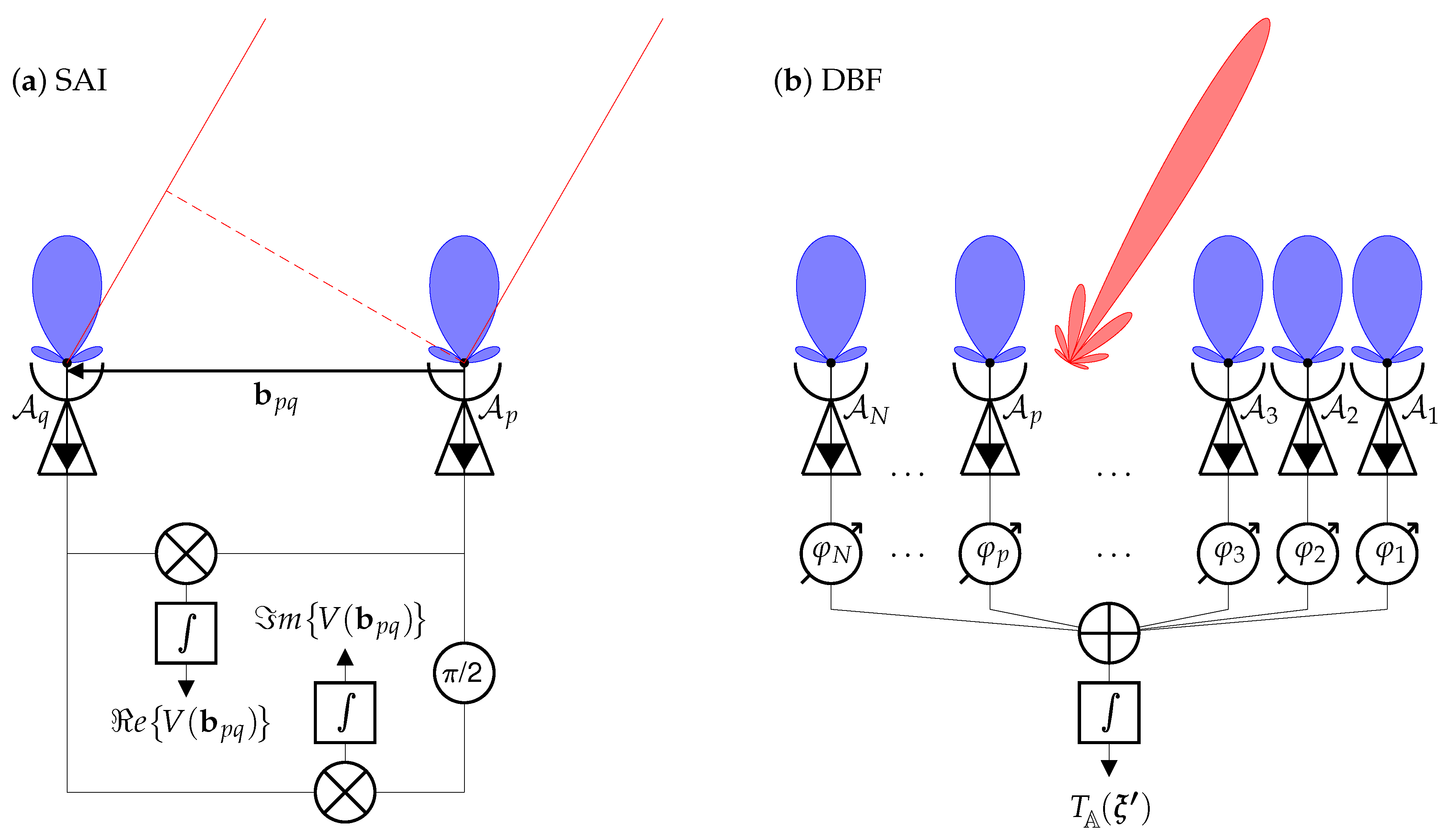
In imaging radiometers using SAI, the signals collected by the elementary antennas are combined pairwise, as illustrated in Figure 1. In actuality, these sensors measure the correlation between the signals collected by antenna pairs, yielding samples of the coherence function, also termed complex visibilities, of the brightness temperature distribution of the observed scene [4].

Without polarimetric considerations [14], and regardless of the decorrelation effects that can be reduced with sub-band decomposition [15] when the narrow-band conditions are not satisfied [16], the complex visibility $V_{pq}\equiv V\left({\mathbf{b}}_{pq}\right)$ for a pair of antennas ${\mathcal{A}}_p$ located in ${\mathbf{r}}_p$ and ${\mathcal{A}}_q$ in ${\mathbf{r}}_q$ is given by:

$${\displaystyle V\left({\mathbf{b}}_{pq}\right)=\frac{1}{\sqrt{{\Omega }_p{\Omega }_q}}\int \underset{\parallel \mathit{\xi }\parallel \le 1}{\int }{\mathcal{F}}_p^{\phantom{\ast }}\left(\mathit{\xi }\right){\mathcal{F}}_q^{\ast }\left(\mathit{\xi }\right)e^{{\displaystyle {\displaystyle -2\mathrm{j}\pi \frac{{\mathbf{b}}_{pq}·\mathit{\xi }}{{\lambda }_o}}\phantom{\frac{a}{\lambda }}}}\frac{T\left(\mathit{\xi }\right)d\mathit{\xi }}{\sqrt{1-{\parallel \mathit{\xi }\parallel }^2}}}$$

(1)

where ${\mathbf{b}}_{pq}\equiv {\mathbf{r}}_q-{\mathbf{r}}_p$ is the baseline vector associated with the two antennas ${\mathcal{A}}_p$ and ${\mathcal{A}}_q$, the components ${\xi }_1=sin\theta cos\varphi$, ${\xi }_2=sin\theta sin\varphi$, and ${\xi }_3=cos\theta$ of the angular position variable $\mathit{\xi }$ are direction cosines ($\theta$ and $\varphi$ are the traditional spherical coordinates), ${\mathcal{F}}_p\left(\mathit{\xi }\right)$ and ${\mathcal{F}}_q\left(\mathit{\xi }\right)$ are the normalized voltage patterns of the antennas ${\mathcal{A}}_p$ and ${\mathcal{A}}_q$ with equivalent solid angles ${\Omega }_p$ and ${\Omega }_q$, as defined by Equations (2)–(24) in [17], $T\left(\mathit{\xi }\right)$ is the brightness temperature distribution of the observed scene, and ${\lambda }_o$ is the central wavelength of observation.

As the geometrical delay in the far-field approximation between the point from the direction $\mathit{\xi }$ at the brightness temperature $T\left(\mathit{\xi }\right)$ and the two antennas ${\mathcal{A}}_p$ and ${\mathcal{A}}_q$ is nothing but the scalar product $({\mathbf{b}}_{pq}·\mathit{\xi })/c$, relation (1) can be written with:

$$\frac{{\mathbf{b}}_{pq}·\mathit{\xi }}{{\lambda }_o}={\nu }_o[{\tau }_p\left(\mathit{\xi }\right)-{\tau }_q\left(\mathit{\xi }\right)]$$

(2)

where ${\nu }_o\equiv c/{\lambda }_o$ is the central frequency of observation and ${\tau }_p\left(\mathit{\xi }\right)-{\tau }_q\left(\mathit{\xi }\right)$ is the time delay between the two elementary antennas and every point in the direction $\mathit{\xi }$.

According to a recent revisit of (1), accounting for the mutual coupling between elementary antennas, the brightness temperature distribution $T\left(\mathit{\xi }\right)$ has to be substituted with the difference $T\left(\mathit{\xi }\right)-T_r$, where $T_r$ is the physical temperature of the receivers [18]. In any case, this constant term does not affect the zero-spacing baselines and it can be removed by measuring a flat target [19]. As a consequence, without any loss of generality, after discretization of the integral found in (1) over an appropriate sampling grid in the direction cosines domain [20], the relationship between the complex visibilities and the brightness temperature distribution of the scene under observation can be written in the algebraic form:

$$V=\underset{\mathrm{sai}}{\mathbf{G}}T$$

(3)

where $\underset{\mathrm{sai}}{\mathbf{G}}$ is the linear modeling matrix of the imaging radiometer using SAI.

2.2. Digital Beam Forming

For DBF imaging radiometers, the signals collected by the elementary antennas are combined all together [8], as illustrated in Figure 1. In actuality, these sensors measure the antenna temperature (see Equation (2-144) in [17], for example) seen by the entire array $\mathbb{A}$, so that all the elementary antennas $\mathcal{A}$ of the collection are simultaneously involved.

Without polarimetric considerations [10] here as well, and disregarding decorrelation effects that can be again reduced with spectral sub-banding [21], the antenna temperature $T_{\mathbb{A}}^{\phantom{\ast }}\left({\mathit{\xi }}^{\prime }\right)$ from the pointing direction ${\mathit{\xi }}^{\prime }$ is given by:

$${\displaystyle T_{\mathbb{A}}^{\phantom{\ast }}\left({\mathit{\xi }}^{\prime }\right)=\frac{1}{\Omega \left({\mathit{\xi }}^{\prime }\right)}\int \underset{\parallel \mathit{\xi }\parallel \le 1}{\int }{\left|\sum _{p=1}^N{\mathcal{F}}_p\left(\mathit{\xi }\right)e^{{\displaystyle {\displaystyle -2\mathrm{j}\pi \frac{{\mathbf{r}}_p·(\mathit{\xi }-{\mathit{\xi }}^{\prime })}{{\lambda }_o}}\phantom{\frac{a}{\lambda }}}}\right|}^2\frac{T\left(\mathit{\xi }\right)d\mathit{\xi }}{\sqrt{1-{\parallel \mathit{\xi }\parallel }^2}}}$$

(4)

where ${\phi }_p\left({\mathit{\xi }}^{\prime }\right)\equiv +2\pi ({\mathbf{r}}_p·{\mathit{\xi }}^{\prime })/{\lambda }_o$ is the phase applied to the signal captured by antenna ${\mathcal{A}}_p$ to steer the beam of $\mathbb{A}$ in the direction ${\mathit{\xi }}^{\prime }$ (see Equations (9) and (10) in [13], for example) and $\Omega \left({\mathit{\xi }}^{\prime }\right)$ is the equivalent solid angle of the antenna array pattern thus formed when pointing in that direction.

Here again, on introducing the propagation times from the points in the directions $\mathit{\xi }$ and ${\mathit{\xi }}^{\prime }$ to the antenna ${\mathcal{A}}_p$, relation (4) can be written with:

$$\frac{{\mathbf{r}}_p·(\mathit{\xi }-{\mathit{\xi }}^{\prime })}{{\lambda }_o}={\nu }_o[{\tau }_p\left(\mathit{\xi }\right)-{\tau }_p\left({\mathit{\xi }}^{\prime }\right)].$$

(5)

Contrary to SAI imaging radiometers whose modeling Equation (1) using (2) reveals a dependency on the time delay between two different antennas from any direction, Equations (4) and (5) show that imaging radiometers using DBF are sensitive to the time delay between two different directions for any antenna.

Finally, here again, without any loss of generality relation (4) is written in the algebraic form:

$$T_{\mathbb{A}}^{\phantom{\ast }}=\underset{\mathrm{dbf}}{\mathbf{G}}T$$

(6)

where $\underset{\mathrm{dbf}}{\mathbf{G}}$ is the linear modeling matrix of the imaging radiometer using DBF.

2.3. Array Factor and Array Pattern

The array factor [22] of the array $\mathbb{A}$ is nothing but the exponential sum over the N elementary antennas:

$$AF(\mathit{\xi },{\mathit{\xi }}^{\prime })=\sum _{p=1}^N{e}^{{\displaystyle {\displaystyle -2\mathrm{j}\pi \frac{{\mathbf{r}}_p·(\mathit{\xi }-{\mathit{\xi }}^{\prime })}{{\lambda }_o}}\phantom{\frac{a}{\lambda }}}}.$$

(7)

The reader may find definitions with weights $w_p$ in the discrete sum, such as in Equations (2.3) and (2.4) in [23], which might be useful for making some trade-offs in the properties of the antenna array. These weights are not included here, or they are all set to 1, so that the maximum value of the array factor, which is at the peak of the main beam of $AF(\mathit{\xi },{\mathit{\xi }}^{\prime })$ when $\mathit{\xi }={\mathit{\xi }}^{\prime }$ for all p in (7), is here equal to N, according to Equation (2.5) in [23]. According to the wording of [8], Equations (4) and (7) refer to “classical beamforming” (also called “uniform beamforming”) in contrast with “optimum beamforming” (also called “weighted beamforming”), where appropriate weights are the result of an optimization process in the design of the antenna array which aims, for some, at improving the signal-to-noise ratio, and, for others, at reducing the level of the side-lobes. As stated in the introduction, the aim of this contribution is not to make such an optimization, it is just to compare the two paradigms under the same conditions from the algebraic point of view.

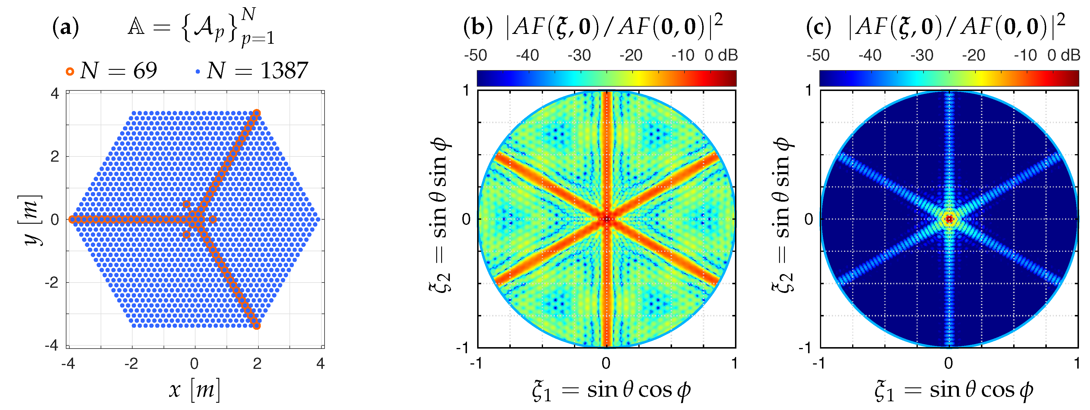
Before entering into the details of this comparison, it is necessary to stress the nature of the antenna array, as the reader may be familiar with dense arrays but less with sparse ones. An interesting study on the impact of dense versus sparse antenna arrays has already been performed by radio astronomers [24]. To concretely illustrate this impact in Earth remote sensing, we consider here the case of the antenna array of SMOS which falls into the category of sparse antenna arrays with its 69 elementary antennas regularly spaced every $0.875{\lambda }_o\simeq 18.56$ cm on the three arms of a Y. Conversely, to study the case of a dense array, let us consider a hexagonal array with the same dimensions but filled with 1387 elementary antennas and with the same spacing (such a dense antenna array can be found in Figure 2.24a in [23]). These arrays are shown in Figure 2 together with their array factor when they point into the direction ${\mathit{\xi }}^{\prime }=(0,0)$. As expected, in both cases, ${\left|AF(\mathit{\xi },\mathbf{0})\right|}^2$ exhibits a main beam centered in $\mathit{\xi }=(0,0)$ and has 6 tails spreading out from it. As a consequence of the sparsity of the antenna array, the main beam of ${\left|AF(\mathit{\xi },\mathbf{0})\right|}^2$ is wider for SMOS than for the dense hexagonal array: $0.0355$ rad versus $0.0299$ rad. Likewise, the side-lobes of ${\left|AF(\mathit{\xi },\mathbf{0})\right|}^2$ have a higher level for SMOS than for the dense hexagonal array: $-7.2$ dB versus $-19$ dB with respect to the peak value.

When the patterns of every elementary antenna are identical, the array pattern of $\mathbb{A}$ is simply the product of the array factor (7) with the element pattern (see Equation (14) in [13]). This is not the case of the SMOS antenna array, as these patterns vary from one elementary antenna to the other [25]. As a consequence, according to Equation (13) in [13], the power pattern of the antenna array $\mathbb{A}$ when pointing in the direction ${\mathit{\xi }}^{\prime }$ is given by:

$$|\mathbb{F}(\mathit{\xi },{\mathit{\xi }}^{\prime }){|}^2={\left|\sum _{p=1}^N{\mathcal{F}}_p\left(\mathit{\xi }\right)e^{{\displaystyle {\displaystyle -2\mathrm{j}\pi \frac{{\mathbf{r}}_p·(\mathit{\xi }-{\mathit{\xi }}^{\prime })}{{\lambda }_o}}\phantom{\frac{a}{\lambda }}}}\right|}^2.$$

(8)

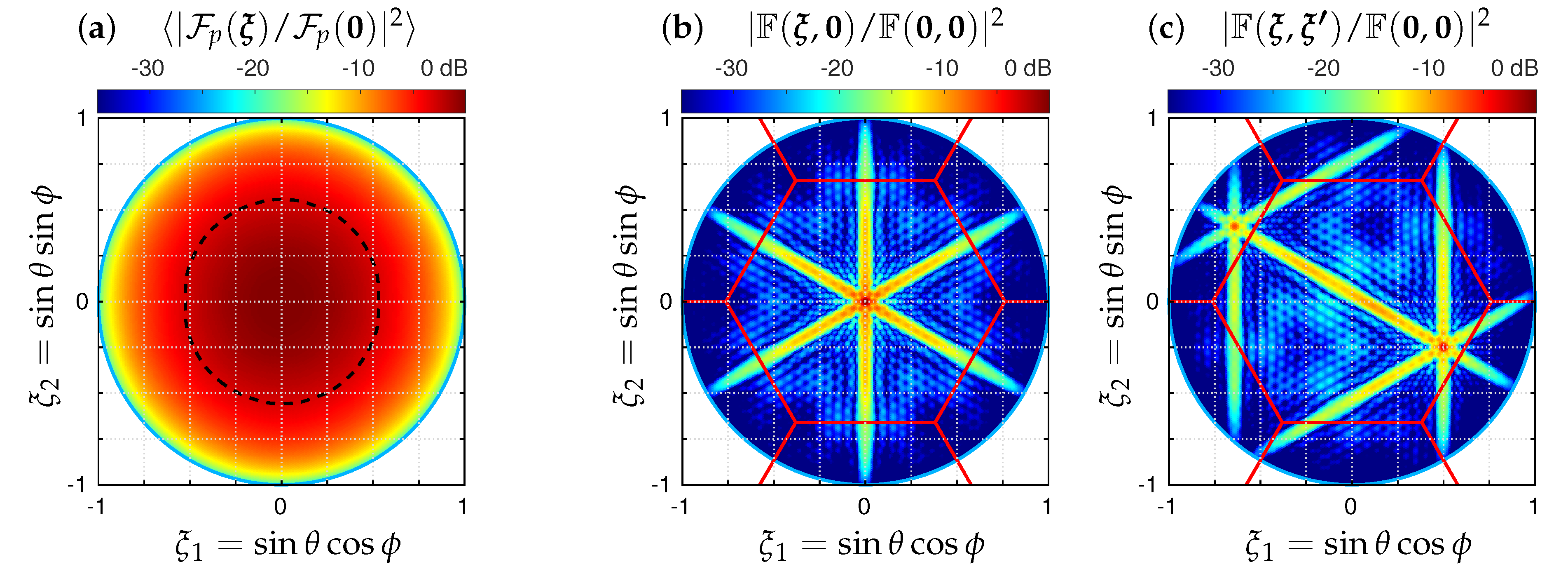
Referring back to the antenna array of SMOS, two examples of such power patterns are compared to the average power pattern of the 69 elementary antennas in Figure 3 when the antenna array points naturally into the boresight direction ${\mathit{\xi }}^{\prime }=(0,0)$ and when it points off-boresight into the direction ${\mathit{\xi }}^{\prime }=(0.5,-0.25)$, thanks to appropriate phases ${\phi }_p\left({\mathit{\xi }}^{\prime }\right)$ steering the beam of the array in that direction. Despite the width of the elementary power patterns (about ${65}^{\circ }$), the array power pattern has quite a narrow beam (about $2^{\circ }$). However, here again, as illustrated in Figure 2, the sparsity of the Y-shaped antenna array is responsible for the high level of the side-lobes. Finally, it is worth noting the attenuation caused by the element power patterns, which varies from one pointing direction ${\mathit{\xi }}^{\prime }$ to another. One should also observe the field aliasing (or the grating lobes) due to the spacing between the elementary antennas together with the geometry of the array. As the spacing between the antennas is here equal to $0.875{\lambda }_o$ and the underlying sampling grid is an hexagonal one, the synthesized field of view is an hexagon and its extension from side to side is equal to $2/\sqrt{3}/0.875\simeq 1.32$ rad, according to Equation (5) in [26].

2.4. On the Need for Inversion

Equations (3) and (6) are algebraically very similar, but they provide very different products because the modeling Equations (1) and (4) are different. SAI products are samples of the complex visibility function $V\left({\mathbf{b}}_{pq}\right)$ for a finite set of baselines ${\mathbf{b}}_{pq}$ spanning the so-called experimental frequency coverage [4]. With DBF, the situation is much simpler because these products are antenna temperatures $T_{\mathbb{A}}^{\phantom{\ast }}\left({\mathit{\xi }}^{\prime }\right)$ as a function of the pointing direction ${\mathit{\xi }}^{\prime }$ of the synthetic beam. As outlined in Section 1, in either case, the final goal is to synthesize a high-resolution brightness temperature map of the observed scene $T\left(\mathit{\xi }\right)$. With SAI concept, the only way to obtain such a map is to invert relation (3) with the aid of a computer. Depending on the pointing directions, DBF products can already be organized similar to a brightness temperature map of the observed scene. The question therefore arises whether an inversion of (6) is necessary, or not.

The answer depends on the antenna array and on its array factor. Substituting for (8) into (4) leads to

$${\displaystyle T_{\mathbb{A}}^{\phantom{\ast }}\left({\mathit{\xi }}^{\prime }\right)=\frac{1}{\Omega \left({\mathit{\xi }}^{\prime }\right)}\int \underset{\parallel \mathit{\xi }\parallel \le 1}{\int }{\left|\mathbb{F}(\mathit{\xi },{\mathit{\xi }}^{\prime })\right|}^2\frac{T\left(\mathit{\xi }\right)d\mathit{\xi }}{\sqrt{1-{\parallel \mathit{\xi }\parallel }^2}}}$$

(9)

which is nothing but the definition of the antenna temperature of Equation (1) in [10], here when all the elementary antennas of $\mathbb{A}$ point in the direction ${\mathit{\xi }}^{\prime }$. As a consequence, inasmuch as the angular position variables $\mathit{\xi }$ and ${\mathit{\xi }}^{\prime }$ belong to the same sampling grid in the direction cosines domain, the antenna temperature map $T_{\mathbb{A}}^{\phantom{\ast }}\left({\mathit{\xi }}^{\prime }\right)$ is exactly the convolution of the modified brightness temperature distribution $T\left(\mathit{\xi }\right)/\sqrt{1-{\parallel \mathit{\xi }\parallel }^2}$ with the power pattern of the antenna array $|\mathbb{F}(\mathit{\xi },{\mathit{\xi }}^{\prime }){|}^2$. As long as a convolution relation is identified, it is natural to question the deconvolution of such a map to improve the angular resolution and/or to clean it from spurious effects such as those induced by side lobes, for example, and/or to remove the attenuation caused by the element power patterns, as illustrated in Figure 3. Of course, the question does not arise for any antenna array with thousands of elementary antennas as is the case with the stations of SKA in radio astronomy [7] or with the dense and regularly filled arrays used for mobile communications [27] or with radar systems [28]. However, as illustrated in Figure 2, the question is relevant for the sparse arrays, such as the SMOS Y-shaped array, and therefore for the hexagonal array currently studied by the European Space Agency (ESA) [29] or for the cross-shaped array investigated by the French space agency (CNES) [30]. Finally, as exemplified in Figure 3, this convolution kernel varies from one pointing direction ${\mathit{\xi }}^{\prime }$ to another in the synthesized field of view, making deconvolution more complicated [31]. Even if the attenuation by the element power patterns from the center to the edge of the synthesized field of view was the only issue, as soon as these patterns are not identical but vary from one elementary antenna to the other (and depending on the final required accuracy), removing this effect cannot be reduced to a simple division by an average power pattern; it requires an appropriate and regularized inversion.

3. Regularized Inversion

As discussed in the previous section, whatever the paradigm, data provided by an antenna array have to be inverted in order to synthesize an estimate of the brightness temperature distribution of the observed scene. Although it is not the subject of this note, referring back to the combination of the signals kept by the elementary antennas, pairwise in SAI and all together with BDF, it could be mentioned that these are not the only ways to combine those signals. In actuality, they can also be combined by triplets [32] and more generally by any number over closed circuits of antennas [33]; however, in any case, the need for an inversion is still present and an analysis similar to the one presented here can be performed with the appropriate modeling operators.

3.1. Singular Values

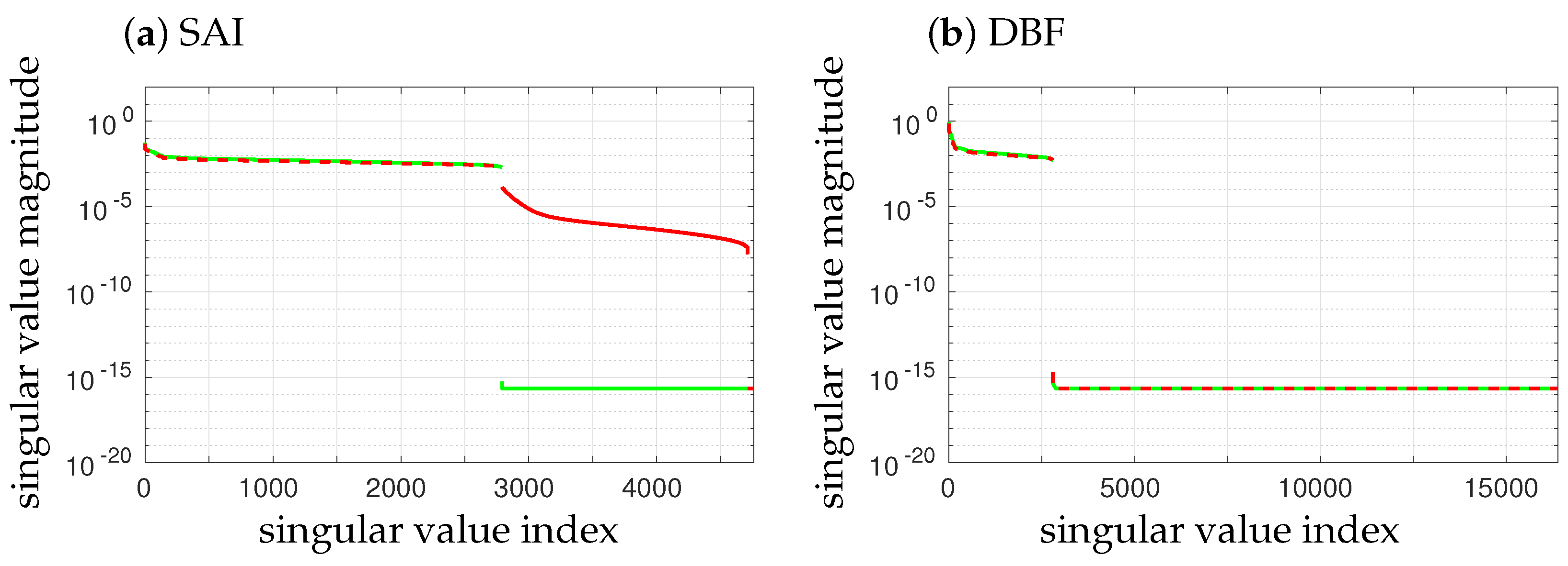
Singular values of a matrix play an important role in numerical linear algebra because they can be used to determine the effective rank of that matrix (singular values beyond a significant gap being numerically equivalent to zero) [34]. Shown in Figure 4 are the singular values of the modeling matrices for the SMOS Y-shaped antenna array when the signals measured by the 69 elementary antennas are processed according to the SAI concept or according to the DBF one. Owing to the choice made for the sampling grid in the direction cosines domain, in both cases, the number of columns of the modeling matrix is equal to ${128}^2$ = 16,384, which is the baseline for the SMOS L1 processor [35]. As detailed in [20], this number of pixels in the synthesized field of view is the minimum power of 2 to guarantee the Shannon sampling conditions with regards to the extension of the frequency coverage of the antenna array. Whatever the paradigm, using more pixels makes the inversions more complicated from the numerical implementation point of view without adding any information. Referring back to the modeling Equations (1) and (4), the case shown in green in Figure 4 of a unique voltage pattern $\mathcal{F}\left(\mathit{\xi }\right)$ for every elementary antenna ${\mathcal{A}}_p$ of the array $\mathbb{A}$ is an ideal situation that cannot be reached. Indeed, manufacturing of elementary antennas and constraints associated with embedding into an antenna array result in a disparity of the elementary patterns after accommodation, an actual situation shown in red in Figure 4.

With regards to SAI and to SMOS, the number of lines of the modeling matrix (3) is equal to the number of visibilities in the so-called “all LICEF mode” [36]. With an array populated with 69 antennas, this number is therefore equal to $69+69(69-1)=4761$. However, only few of these lines are independent as a consequence of redundant baselines. For SMOS, when accounting for the redundant baselines along the three arms of the Y-shaped array, this number of Fourier frequencies in the star-shaped frequency coverage is equal to 2791. This property clearly appears in the distribution of the singular values of the modeling matrix (3) because there is a first group of 2791 singular values well-separated from the others, especially for an instrument equipped with identical elementary antennas.

With regards to DBF with SMOS, the number of lines of the modeling matrix (6) is equal to the number of pointing directions in the synthesized field of view. For SMOS, this number has been set to ${128}^2$ = 16,384. Surprisingly enough, here again, the number of independent lines is equal to 2791. This property clearly appears in the distribution of the singular values of the modeling matrix (6) as there is again a first group of 2791 singular values well-separated from the others, whatever the diversity of the antennas.

As a consequence, in both paradigms, the effective rank of the modeling matrix is equal to the number of Fourier frequencies in the star-shaped frequency coverage of the antenna array of SMOS. Whatever the concept, these imaging radiometers are band-limiting devices. This property is easily understood for SAI because the complex visibility function is sampled only for baselines ${\mathbf{b}}_{pq}$ spanning the frequency coverage of the antenna array [20]. However, it is not evidence for DBF, so it will be illustrated with numerical simulations in the last section of this note. From the algebraic point of view, the modeling matrix (3) is very sensitive to the disparity of the elementary antennas patterns which can jeopardize this interesting property due to the loss of redundant baselines as, if the geometry is respected, the elements are too different to allow redundancy. On the contrary, the modeling matrix (6) is far less sensitive to this disparity, thus strictly preserving the rank property.

3.2. Retrieved Maps

As a consequence of rank-deficient modeling matrices [37], the corresponding inverse problems have to be regularized in order to provide unique solutions to the linear systems (3) and (6). For obvious reasons of comparison between the two paradigms, the same regularization is implemented in either case. Otherwise, the differences that might be observed could be attributed to the regularization itself and not to the modeling matrix (and, finally, not to the observational principle which varies from one concept to the other because the combination of the signals kept by the elementary antennas is not the same). Among the many regularization methods that can be found in the literature, the minimum-norm one is widely used in SAI [38]:

$$T_r=\underset{T}{min}{\parallel T\parallel }^2\mathrm{s}.\mathrm{t}.\underset{\mathrm{sai}}{\mathbf{G}}T=V.$$

(10a)

Numerical implementations are available in many algorithmic libraries and with many programming languages. The extension to DBF does not raise any problem and it is straightforward:

$$T_r=\underset{T}{min}{\parallel T\parallel }^2\mathrm{s}.\mathrm{t}.\underset{\mathrm{dbf}}{\mathbf{G}}T=T_{\mathbb{A}}^{\phantom{\ast }}.$$

(10b)

In both cases, the $T_r$ map is obtained through the computation of the pseudo-inverse of the modeling matrix:

$$T_r={\underset{\mathrm{sai}}{\mathbf{G}}}^{+}V,$$

(11a)

and

$$T_r={\underset{\mathrm{dbf}}{\mathbf{G}}}^{+}{T}_{\mathbb{A}}^{\phantom{\ast }}.$$

(11b)

Referring back to Figure 4, in either case, ${\mathbf{G}}^{+}$ is computed with the aid of a truncated singular values decomposition of $\mathbf{G}$, where only the 2791 largest singular values are kept during the inversion [39]. As a consequence, ${\mathbf{G}}^{+}\mathbf{G}$ is no longer equal to the identity matrix and a reconstruction floor error has to be expected [40]. However, referring back again to Figure 4, there might be a difference between the two retrieved maps (11a) and (11b), owing to the role played by the singular values discarded before the inversion of $\mathbf{G}$. It is necessary then to assess the impact of this difference. Only numerical simulations can address this point, and this is the purpose of the next section.

Finally, in order to filter out the Gibbs effects observed in the direction cosines domain caused by the sharp cut-off in the frequency domain due to the limited extent of the frequency coverage of the antenna array, $T_r$ has to be damped by an appropriate apodization (or windowing) function W [26]:

$${\mathcal{T}}_r=W\star T_r,$$

(12)

where ⋆ is the convolution operator. This map has to be compared to

$$\mathcal{T}=W\star T,$$

(13)

which is the “ideal” temperature map to be reconstructed and apodized with the same window W, and not to T, which is not at the same angular resolution. Although sometimes it is interesting to compare $T_r$ and T at different levels of resolution in order to emphasize differences from this point of view, here it is clearly not the case, as the next section will illustrate identical performances of SAI and DBF in terms of angular resolution. This is why, as announced in the introduction, this note aims at comparing the two paradigms in terms of the overall reconstruction error by comparing ${\mathcal{T}}_r$ to $\mathcal{T}$, without being disturbed by such resolution aspects that, moreover, do not have to be considered here.

4. Numerical Simulations and Comparison

Currently, there is no sparse antenna array observing the Earth, except SMOS, which is using SAI and not DBF. It is therefore unfortunately not possible to confront these two paradigms with experimental results. However, this comparison can be achieved with the aid of numerical simulations conducted with the most up-to-date instrument modeling of the SMOS antenna array, including the diversity of the elementary patterns. This is exactly what is presented in this section, where all the numerical simulations have been performed for the SMOS Y-shaped antenna array with the 69 elementary patterns measured prior to launch in an anechoic chamber [41]. For every scene observed by the instrument, complex visibilities have been simulated according to (1), and antenna temperatures according to (4). They have been inverted according to (11) and apodized according to (12) with a Blackman window, which is the baseline of the SMOS L1 processor [35]. The impact of the difference between the two distributions of singular values shown in Figure 4 is assessed here spatially and angularly at the level of the reconstruction floor error. The comparison between the two concepts is completed with numerical results showing no difference with regards to the radiometric sensitivity of the reconstruction process and to the angular resolution of the retrieved maps.

4.1. Fresnel Scene

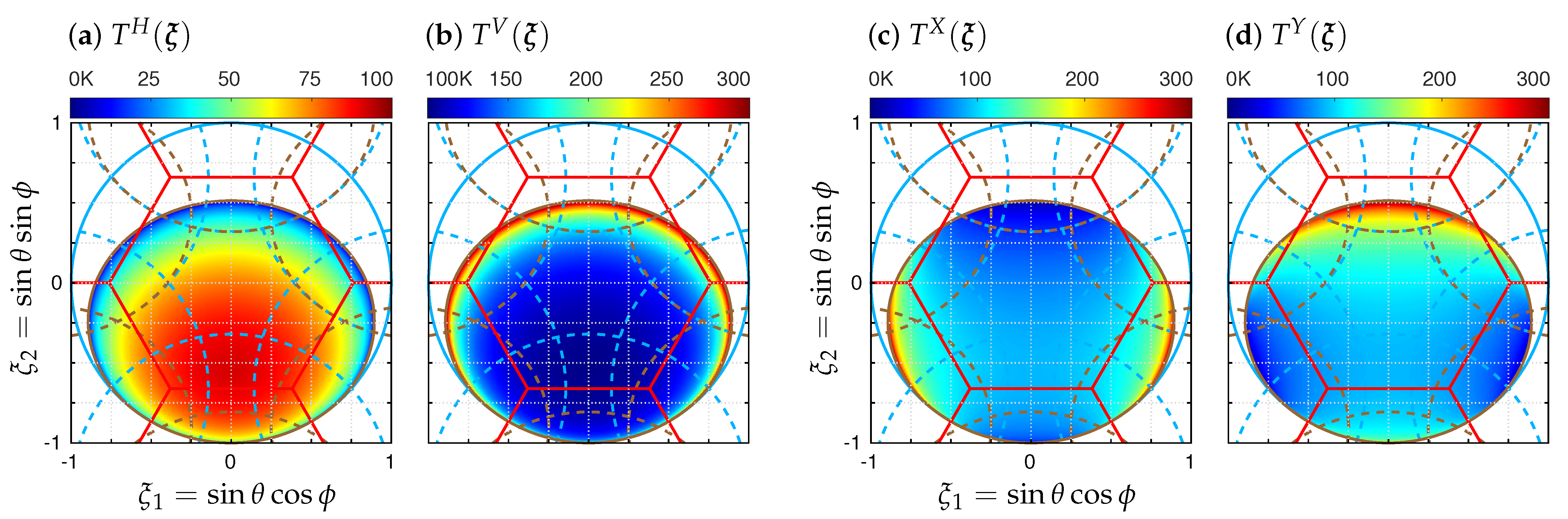
Shown in Figure 5 are the brightness temperature distributions $T^H$ and $T^V$ of a typical scene over the ocean in horizontal and vertical polarizations for a smooth sea surface (Equation (5) in [42]) with the Klein and Swift model for the dielectric constant [43]. A rotation angle is applied to $T^H$, $T^V$, and $T^{HV}$ (here set to 0 K) for calculating the corresponding brightness temperatures distributions $T^X$, $T^Y$, and $T^{XY}$ at instrument level, according to Equation (1) in [42]. As the contribution from the deep sky is removed in the SMOS L1 processor [35], it is not shown in Figure 5 for practical reasons.

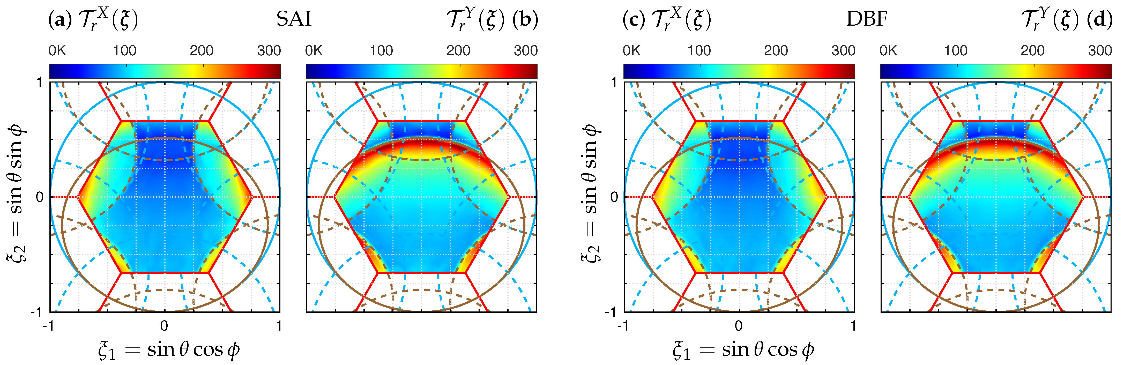
Shown in Figure 6 are the brightness temperature maps ${\mathcal{T}}_r$ retrieved at instrument level in X and Y polarizations with the two paradigms. From a qualitative point of view, there is no significant difference between those obtained with SAI from complex visibilities and those retrieved from antenna temperatures with DBF, including in the aliases of the hexagonal synthesized FOV (field of view).

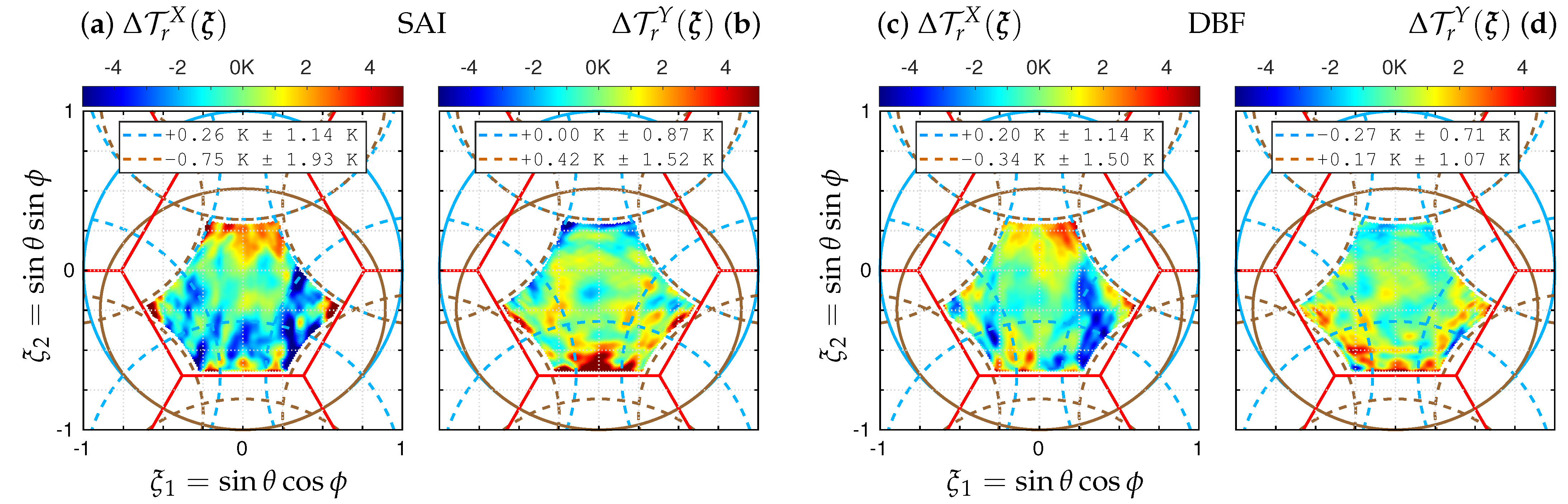
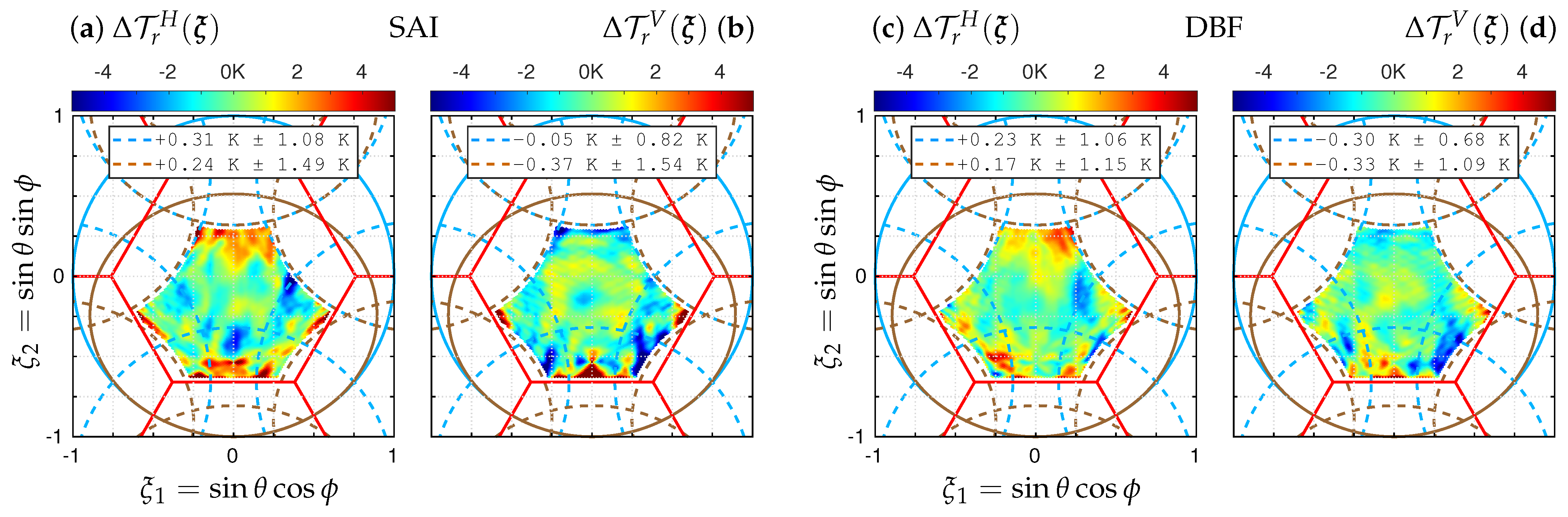
The error maps $\Delta {\mathcal{T}}_r\equiv {\mathcal{T}}_r-\mathcal{T}$ of the retrieved brightness temperature maps with the two paradigms are shown in Figure 7 at instrument level in X and Y polarizations and in Figure 8 at ground level in H and V polarizations. Whatever the polarization, one can immediately observe a difference between the two paradigms on the spatial distribution of this error in the synthesized FOV. Spatial bias and standard deviation are given on these figures in the AF-FOV (alias-free field of view) as well as in the EAF-FOV (extended alias-free field of view). The corresponding RMSE (root mean square error) [44] are given in

Table 1. Root mean square errors in the retrieved brightness temperature maps at instrument level in X and Y polarizations and at ground level in H and V polarizations.

	X Polarization		Y Polarization
	AF-FOV	EAF-FOV	AF-FOV	EAF-FOV
SAI	$1.17$ K	$2.07$ K	$0.87$ K	$1.58$ K
DBF	$1.15$ K	$1.54$ K	$0.76$ K	$1.08$ K
	H Polarization		V Polarization
	AF-FOV	EAF-FOV	AF-FOV	EAF-FOV
SAI	$1.12$ K	$1.51$ K	$0.82$ K	$1.59$ K
DBF	$1.09$ K	$1.16$ K	$0.74$ K	$1.14$ K

. In the AF-FOV, the two concepts perform roughly similarly: in every case, the differences are less than $0.1$ K, but still always to the credit of DBF. On the contrary, in the EAF-FOV, the two paradigms perform much differently: whatever the polarization, the RMSEs with DBF are about $0.5$ K below those obtained with SAI.

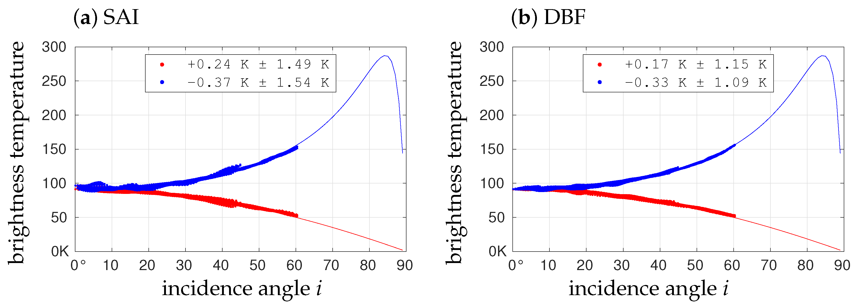
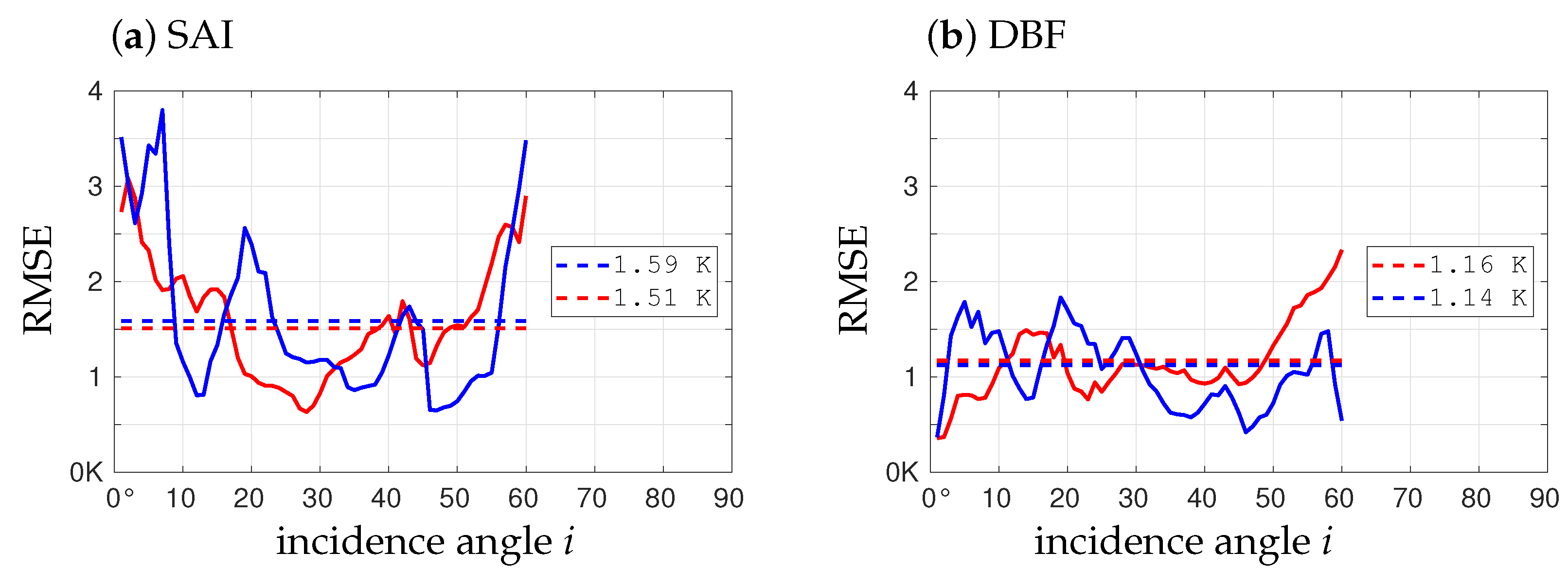
Finally, the variations of the retrieved temperatures ${\mathcal{T}}_r^H$ and ${\mathcal{T}}_r^V$ with the incidence angle at ground level i in the EAF-FOV are shown in Figure 9 and compared to the theoretical profiles at the same resolution in ${\mathcal{T}}^H$ and ${\mathcal{T}}^V$. Oscillations and artifacts clearly appear with SAI, especially at low incidence angles, but not only. On the contrary, they are almost absent, or at least strongly reduced, with DBF. This is confirmed by the RMSE shown in Figure 10, where DBF performs better than SAI in both polarizations, almost at any incidence angle and notably at the lowest ones where the reduction can be as large as 2 K. Moreover, the directional signature of the floor error is less important with DBF than with SAI, as emphasized by the corresponding RMSE profiles, which are flatter with the former paradigm than with the latter one: in the ground incidence angles interval from $0^{\circ }$ to ${60}^{\circ }$, the overall variation range of RMSE is larger than 3 K with SAI, while it is about $1.5$ K with DBF.

4.2. Radiometric Sensitivity

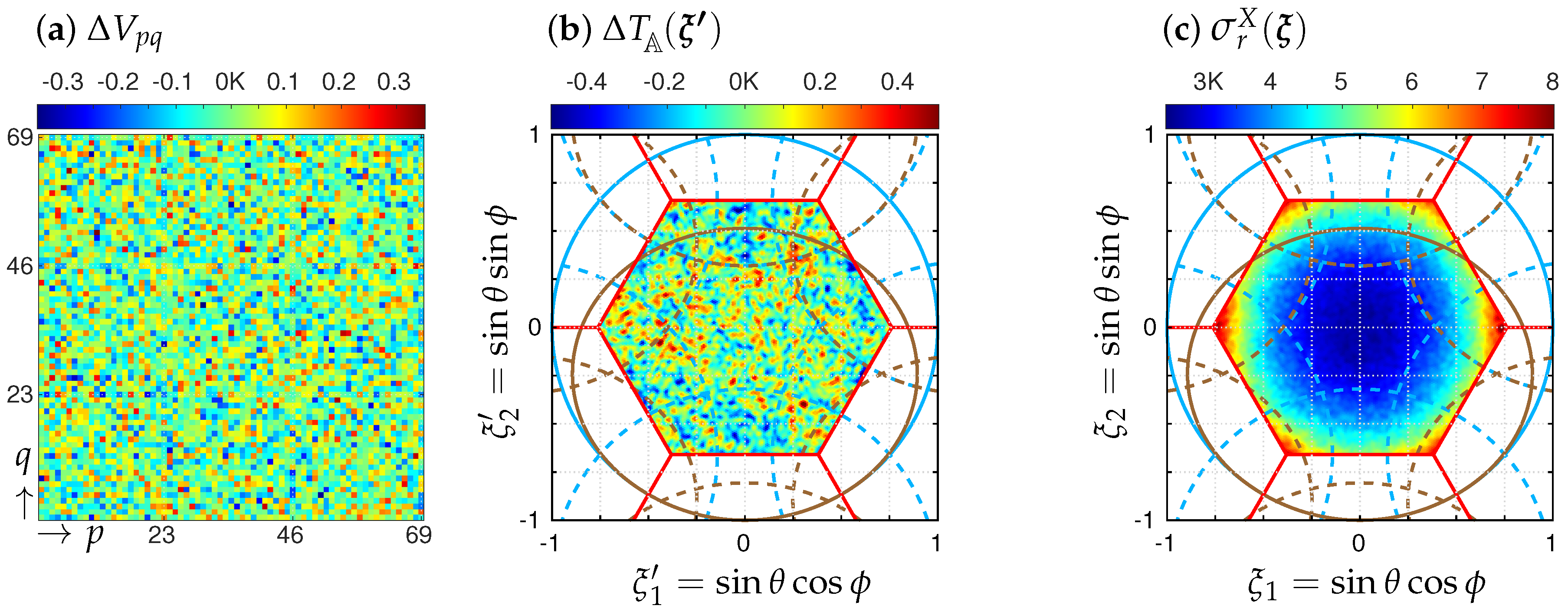
The complex visibilities $V_{pq}$ have been blurred by an additive Gaussian noise $\Delta V_{pq}$ with standard deviation set to $0.1$ K on both the real and the imaginary parts. This value is a typical one for SMOS over the ocean and it corresponds to $T_A=150$ K, $T_R=200$ K, $B=19$ MHz, and ${\tau }_{eff}=1.2/1.81\simeq 0.66$ sec in Equation (12) in [45]. According to SMOS mission requirements [1], the radiometric sensitivity should be about $2.5$ K over the ocean at boresight. This is what is observed in Figure 11, where the estimation of the radiometric sensitivity in the boresight direction $\mathit{\xi }=(0,0)$ is equal to $2.55$ K after 1000 random trials of the additive Gaussian noise. Away from this direction, errors are amplified by the inverse of the antenna radiation pattern times $\sqrt{1-{\parallel \mathit{\xi }\parallel }^2}$ [46].

Thanks to Equation (14) in [10], the same random trials have been used for blurring the antenna temperatures $T_{\mathbb{A}}^{\phantom{\ast }}\left({\mathit{\xi }}^{\prime }\right)$ with an additive Gaussian noise $\Delta T_{\mathbb{A}}^{\phantom{\ast }}\left({\mathit{\xi }}^{\prime }\right)$, so that the comparison from this point of view will not suffer any computational bias. As this Equation does preserve the norm, and because $\Delta V_{pq}$ samples are complex-valued with independent real and imaginary parts, whereas $\Delta T_{\mathbb{A}}^{\phantom{\ast }}\left({\mathit{\xi }}^{\prime }\right)$ are real-valued, according to Equation (5.29) in [47], the standard deviation of $\Delta T_{\mathbb{A}}^{\phantom{\ast }}\left({\mathit{\xi }}^{\prime }\right)$ is here equal to $0.1\sqrt{2}\simeq 0.14$ K, as illustrated in Figure 11. Consequently, the radiometric sensitivity map is identical to that obtained previously in the SAI mode.

4.3. Angular Resolution

The angular resolution of an imaging system is usually defined as its ability to separate two closely spaced identical point sources. The full-width at half-maximum (FWHM) value of the response of the antenna array to a point source [26] is widely used to estimate this angular separation. Referring back to the arguments about the need for the inversion of (6), complex visibilities (1) and antenna temperatures (4) have been simulated and inverted for an observed scene made of a single hot-spot in the very center of the field of view $\mathit{\xi }=(0,0)$, so that the two paradigms can be confronted from the angular resolution point of view by comparing the FWHM of the two retrieved brightness temperature maps $T_r$ as well as that of the antenna temperature map $T_{\mathbb{A}}$.

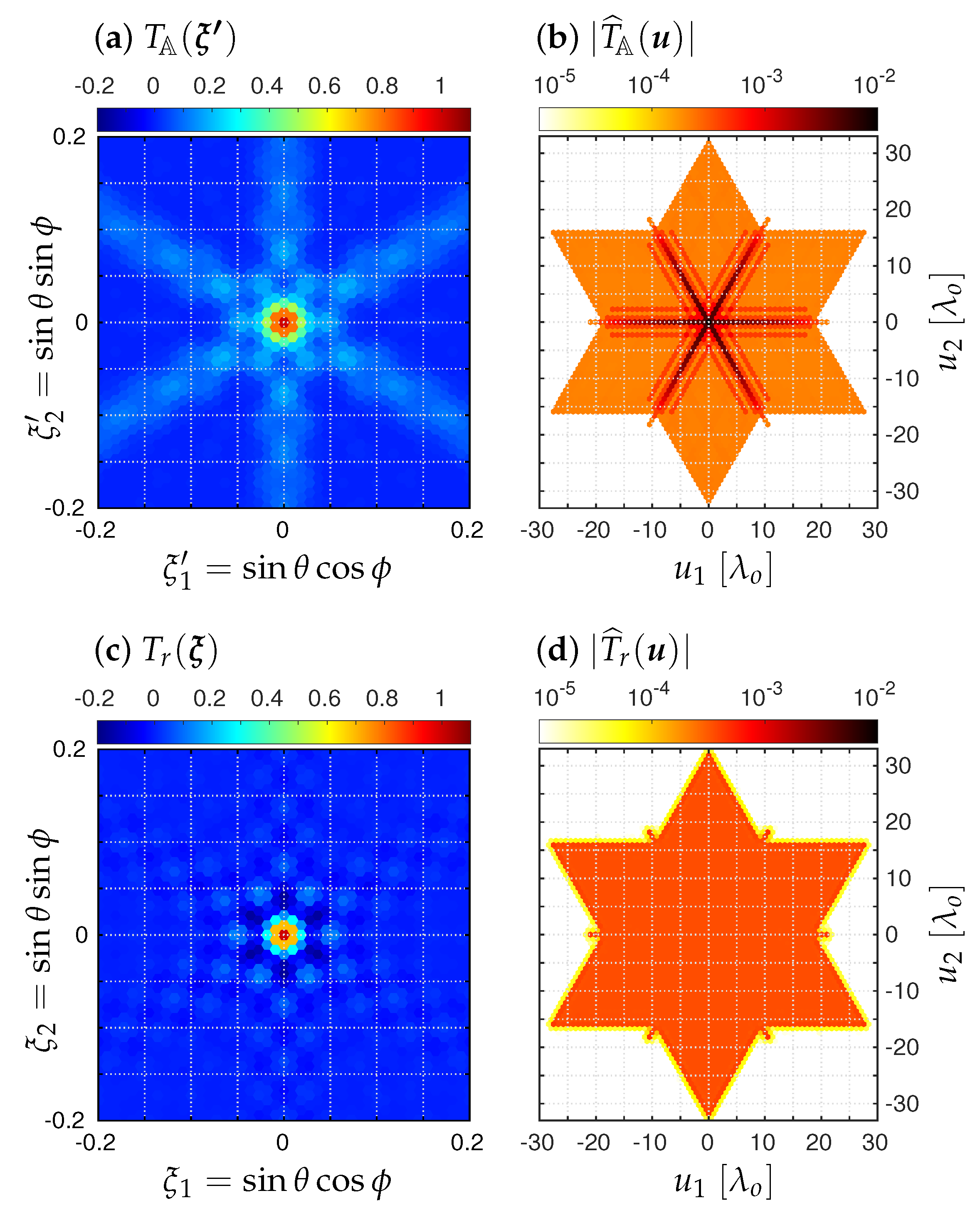
Shown in Figure 12 is the antenna temperature map $T_{\mathbb{A}}\left({\mathit{\xi }}^{\prime }\right)$ normalized to its maximum in ${\mathit{\xi }}^{\prime }=(0,0)$ and the amplitude of its Fourier transform $|{\widehat{T}}_{\mathbb{A}}\left(\mathbf{u}\right)|$ calculated over the dual grid of the hexagonal grid sampling the direction cosines domain [26]. The six tails observed in $T_{\mathbb{A}}\left({\mathit{\xi }}^{\prime }\right)$ with values as high as $0.2$ are caused by the same tails in the power pattern of the antenna array $|\mathbb{F}(\mathit{\xi },{\mathit{\xi }}^{\prime }){|}^2$ shown in Figure 3, because according to (9), they collect energy from the hot-spot even when the antenna array does not point in its direction. With regards to $|{\widehat{T}}_{\mathbb{A}}\left(\mathbf{u}\right)|$, it is worth noting that the energy is limited to the star-shaped frequency coverage of the antenna array. This band-limited property and the associated physical concept of limited resolution of the imaging instrument which has been selected by ESA for being implemented in the SMOS ground segment processor [20] are evident for an interferometer because the complex visibility function is sampled only for baselines ${\mathbf{b}}_{pq}$ spanning the frequency coverage. However, it is not evidence for the DBF paradigm illustrated here. As a consequence of the six-pointed star response to a hot-spot observed in the direction cosines domain at $T_{\mathbb{A}}\left({\mathit{\xi }}^{\prime }\right)$ level, a six-pointed star is also observed in the Fourier domain at $|{\widehat{T}}_{\mathbb{A}}\left(\mathbf{u}\right)|$ level (with a ${90}^{\circ }$ rotation because the two grids are dual one from the other, as detailed in [26]). Also shown in Figure 12 is the normalized brightness temperature map $T_r\left(\mathit{\xi }\right)$ retrieved from that antenna temperature map when inverting (4) according to (11b), as well as the amplitude of its Fourier transform $|{\widehat{T}}_r\left(\mathbf{u}\right)|$. The previous six tails are still present but their impact has been strongly reduced thanks to the regularized inversion. As a consequence, the six-pointed star is no longer observed in the Fourier domain which now exhibits an almost constant energy in the star-shaped experimental frequency coverage. As expected, the same behavior is observed on the brightness temperature map retrieved from the complex visibilities corresponding to the same hot-spot when inverting (1) according to (11a).

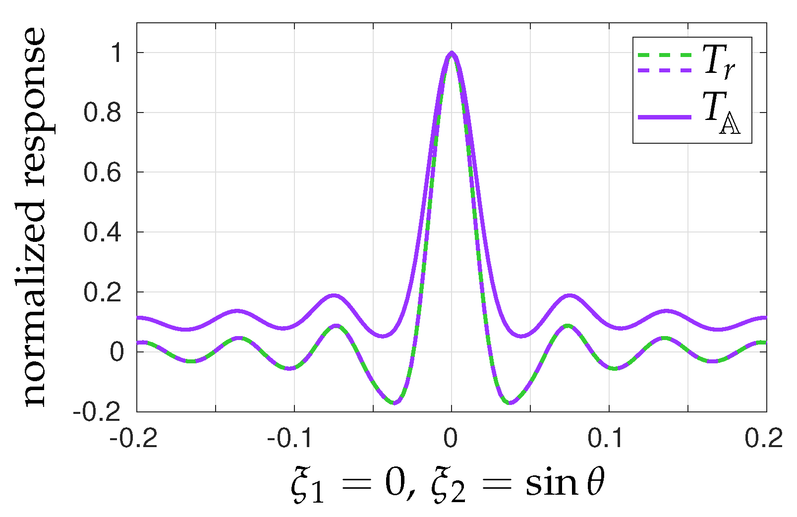
Shown in Figure 13 are cuts along the ${\mathit{\xi }}_2$ axis of the brightness temperature maps $T_r\left(\mathit{\xi }\right)$ retrieved with the two concepts according to (11). It should be kept in mind that at this level of the inversion there is no apodization window, so that the maps are at the highest resolution possible for the instrument. As the two maps are identical, in both cases the FWHM of the normalized response is about $0.0278$ rad which is consistent with the value obtained from the factors of merit listed in Table II of [26]. In order to illustrate again the need for an inversion of the brightness temperature map, the same cut of $T_{\mathbb{A}}\left({\mathit{\xi }}^{\prime }\right)$, which is also not apodized, is reported in the same figure for comparison. As expected, the angular resolution is larger than that obtained with the retrieved maps, since the FWHM of the main beam is here about $0.0355$ rad. Referring back to the maps $T_{\mathbb{A}}\left({\mathit{\xi }}^{\prime }\right)$ and $T_r\left(\mathit{\xi }\right)$ shown in Figure 12, now in the light of the cuts of Figure 13, another effect of the inversion has been to improve the beam efficiency at half-maximum (BEHM) from $25\%$ to $62\%$ [26] by reducing the level of the tails.

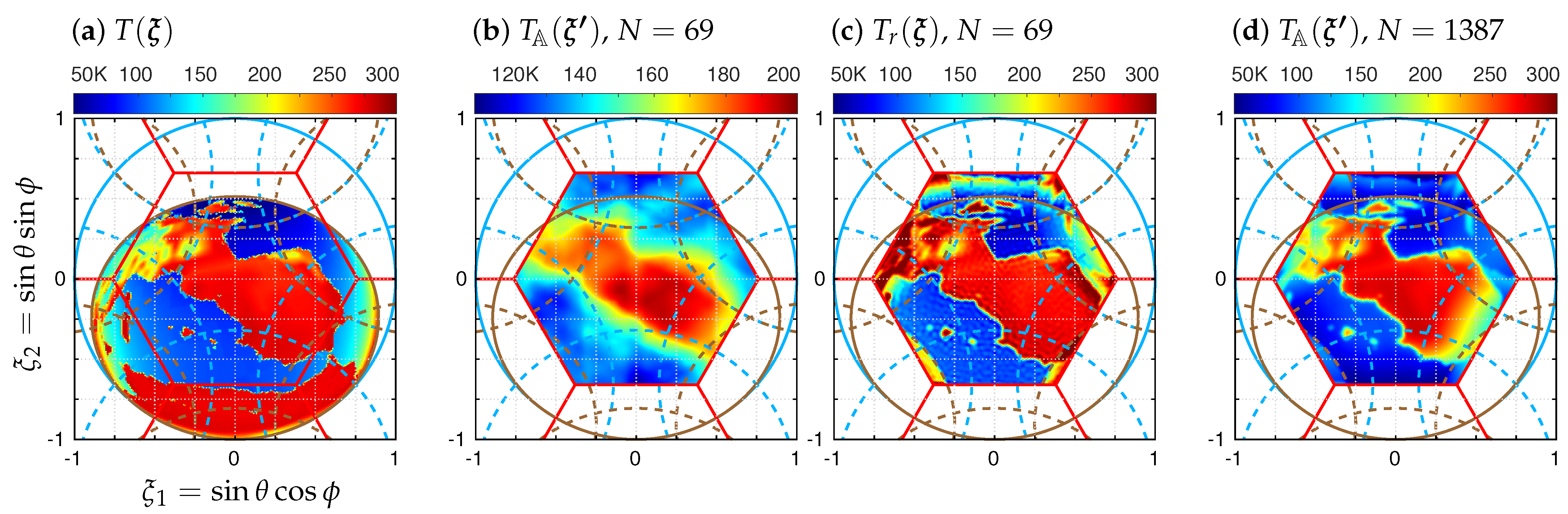
As a consequence, with sparse antenna arrays using DBF, it would be necessary to invert the antenna temperature maps according to (11b) in the same way that there is no alternative but to invert the complex visibilities in SAI according to (11a). As soon as it is the case, it has been clearly shown here that from the angular resolution point of view, there is no difference between the two paradigms. Finally, referring back again to the arguments about the need for inverting the antenna temperature maps, a very last illustration is shown in Figure 14 with a typical scene $T\left(\mathit{\xi }\right)$ over Spain. It shows the comparison between the antenna temperature map $T_{\mathbb{A}}\left({\mathit{\xi }}^{\prime }\right)$ simulated according to (4) for the SMOS Y-shaped array using DBF with 69 elementary antennas; the brightness temperature distribution $T_r\left(\mathit{\xi }\right)$ retrieved from the inversion of this $T_{\mathbb{A}}\left({\mathit{\xi }}^{\prime }\right)$, map according to (11b); and another antenna temperature map simulated for the hexagonal array of Figure 2 using DBF with 1387 elementary antennas. With regards to the angular resolution of these maps, the situation is as clear as the numbers given in Figure 2 and Figure 13. For the SMOS array with only 69 elementary antennas regularly spaced along the three arms of a Y, the angular resolution of the antenna temperature map is about $0.0355$ rad, while it is about $0.0278$ rad for the brightness temperature distribution retrieved from the inversion of this antenna temperature map: the effect of the inversion with (11b) cannot be clearer. Moreover, for those who would still be hesitant to invert the antenna temperature map with the aid of a computer and would prefer to rely on the instrument only, the angular resolution of the antenna temperature map obtained with the dense hexagonal array populated with 1387 elementary antennas is about $0.0299$ rad: it does not even reach the level of resolution of the brightness temperature distribution retrieved from the inversion of the antenna temperature map obtained with SMOS’s sparse array and its 69 elementary antennas. To be complete and honest, it should be mentioned that this comparison does not take into account the radiometric sensitivity that would be, of course, much better with a large number of elementary antennas. However, if the number of elementary antennas for an array observing the deep sky from the Earth’s surface has almost no limit, this is not the case for Earth remote sensing from space, which has strong limits in terms of mass, size, and power consumption, for example, so that one day or another inversion of temperature maps with DBF will have to be taken into account in the scientific and technical trade-offs, as it is with SAI. This is all the more true as the computational cost is not a bottleneck. Indeed, referring back to Figure 4 and to the dimensions of the modeling matrices, the computational cost of (11b) is ${128}^2/4761\simeq 3.5$ longer than that of (11a). However, after 12 years of experience with SMOS, it should be kept in mind that such a basic operation of numerical linear algebra is performed with any algorithmic library in a much shorter time than the integration time of a snapshot (nowadays, a few microseconds on a 10 Gflops floating-point unit compared to a second).

5. Conclusions

Synthetic aperture interferometry (SAI) and digital beam forming (DBF) are two signal processing techniques that are using the same elementary signals collected by an antenna array and are sharing the same goal to produce from them high-resolution images with the aid of the computer. On one hand, SAI is mixing the elementary signals pairwise to estimate the corresponding complex visibilities from the correlation of the two signals. On the other hand, DBF is combining all the elementary signals with a digital beam former to steer the synthesized beam of the array in a given direction and estimate the antenna temperature from that direction.

These two paradigms have been compared from the algebraic point of view with the aid of numerical simulations based upon the SMOS instrument characteristics. The properties of the modeling matrices of these two approaches have been examined. Both are rank-deficient and they have the same effective rank: the number of Fourier frequencies in the star-shaped frequency coverage of the Y-shaped antenna array. This is clearly evidenced with a singular value decomposition where two groups of well-separated singular values are observed. However, in the SAI case, the modeling matrix is very sensitive to the disparity of the elementary antennas patterns which can reduce the gap between these two groups, making the pseudo-inversion more delicate. On the contrary, in the DBF case, the modeling matrix is far less sensitive to this disparity and the gap between the two groups of singular values is preserved, making the pseudo-inversion more robust.

As a consequence of this first difference at modeling matrix level, few differences have been observed and reported at the level of the retrieved brightness temperature maps. From a qualitative point of view, whatever the polarization, the spatial distribution of the reconstruction floor error in the synthesized field of view exhibits interesting differences from one paradigm to the other. From a qualitative point of view, global metrics have shown a significant reduction of the level of this error in every polarization with DBF compared to SAI, especially in the so-called extended alias-free field of view where it could be as large as $0.5$ K. Moreover, with respect to the directional signature of this floor error, it turns out that DBF performs better than SAI at any incidence angle, notably at the lowest ones where the reduction can be as large as 2 K, leading to an almost constant level of floor error over a wide range of incidence angles. Finally, propagation of random Gaussian noise through the reconstruction process of both paradigms has not shown any difference with regards to the final radiometric sensitivity in the synthesized field of view. Likewise, with regards to the angular resolution, the synthesized impulse responses are strictly identical.

It is unfortunate that these conclusions are derived only from simulated data and not from experimental results. The fact remains that currently there is no sparse antenna array observing the Earth except SMOS, which is using only SAI to image the Earth’s surface at L band. On the other hand, there are a few antenna arrays observing the sky with DBF capabilities, but these arrays do not fall into the sparse category. Radio astronomy and Earth remote sensing synthesize different fields of view at different angular resolutions. Moreover, while there is almost no limit to the number of elementary antennas in an antenna array in radio astronomy, Earth remote sensing from space has strong limits (mass, size, power consumption, etc.) that are not compatible with dense and regularly filled arrays with plenty of elementary antennas. This is why, at the time that agencies and industries are conducting preliminary studies for an SMOS follow-on mission, only numerical simulations carried on within the framework of the SMOS mission have been performed to compare these two concepts and to illustrate what the results could have been if the signals kept by the elementary antennas of SMOS had been combined all together for DBF instead of pairwise for SAI. This work has no other claim than that. Calibration and hardware considerations are out of the field of competence of the authors and are left to specialists. Nevertheless, referring back to the introduction and to the place devoted to DBF in radio astronomy, as soon as no major issue is found or encountered in the spatialization of this paradigm, DBF should deserve attention in the studies of future imaging radiometers as an interesting option. This does not mean that DBF is preferable to SAI. This simply means that DBF should be studied as much as SAI, neither more, nor less.

References

- Barré, H.; Duesmann, B.; Kerr, Y.H. SMOS: The mission and the system. IEEE Trans. Geosci. Remote Sens. 2008, 46, 587–593. [Google Scholar] [CrossRef]
- McMullan, K.D.; Brown, M.A.; Martín-Neira, M.; Rits, W.; Ekholm, S.; Lemanczyk, J. SMOS: The payload. IEEE Trans. Geosci. Remote Sens. 2008, 46, 594–605. [Google Scholar] [CrossRef]
- de Rosnay, P.; Rodriguez-Fernandez, N.; Munoz-Sabater, J.; Albergel, C.; Fairbairn, D.; Lawrence, H.; English, S.; Drusch, M.; Kerr, Y.H. SMOS Data Assimilation for Numerical Weather Prediction. In Proceedings of the International Geoscience And Remote Sensing Symposium (IGARSS 2018), Valencia, Spain, 22–27 July 2018. [Google Scholar]
- Thompson, A.R.; Moran, J.W.; Swenson, G.W. Interferometry and Synthesis in Radio Astronomy, 3rd ed.; Springer International Publishing: Cham, Switzerland, 2017. [Google Scholar]
- Thompson, A.R.; Clark, B.G.; Wade, C.M.; Napier, P.J. The Very Large Array. Astrophys. J. Suppl. Ser. 1980, 44, 151–167. [Google Scholar] [CrossRef]
- Padin, S.; Shepherd, M.C.; Cartwright, J.K.; Keeney, R.G.; Mason, B.S.; Pearson, T.J.; Readhead, A.C.S.; Schaal, W.A.; Sievers, J.; Udomprasert, P.S.; et al. The Cosmic Background Imager. Publ. Astron. Soc. Pac. 2002, 114, 83–97. [Google Scholar] [CrossRef] [Green Version]
- Dewdney, P.E.; Hall, P.J.; Schilizzi, R.T.; Lazio, T.J.L.W. The Square Kilometre Array. Proc. IEEE 2009, 97, 1482–1496. [Google Scholar] [CrossRef]
- Van Veen, B.D.; Buckley, K.M. Beamforming: A versatile approach to spatial filtering. IEEE ASSP Mag. 1988, 5, 4–24. [Google Scholar] [CrossRef]
- Ho, T.K.; Feng, J.; Bilawal, F.; Shehab, S.; Trinh, K.T.; Yang, Y.; Rudiger, C.; Walker, J.P.; Karmakar, N.C. Lightweight and Compact Radiometers for Soil Moisture Measurement: A Review. IEEE Geosci. Remote Sens. Mag. 2022, 10, 231–250. [Google Scholar] [CrossRef]
- Bosch-Lluis, X.; Ramos-Pŕez, I.; Camps, A.; Rodriguez-Alvarez, N.; Valencia, E.; Park, H. Common Mathematical Framework for Real and Synthetic Aperture by Interferometry Radiometers. IEEE Trans. Geosci. Remote Sens. 2014, 52, 38–50. [Google Scholar] [CrossRef]
- Bosch-Lluis, X.; Ramos-Pérez, I.; Camps, A.; Rodriguez-Alvarez, N.; Valencia, E.; Marchan-Hernandez, J.F. Description and performance of an L-band radiometer with digital beamforming. Remote Sens. J. 2010, 3, 14–40. [Google Scholar] [CrossRef] [Green Version]
- Duran, I.; Lin, W.; Corbella, I.; Torres, F.; Duffo, N.; Martín-Neira, M. SMOS floor error impact and mitigation on ocean imaging. In Proceedings of the International Geoscience And Remote Sensing Symposium (IGARSS 2015), Milan, Italy, 26–31 July 2015. [Google Scholar]
- Allen, J.L. Array antennas: New applications for an old technique. IEEE Spectr. 1964, 1, 115–130. [Google Scholar] [CrossRef]
- Camps, A.; Corbella, I.; Torres, F.; Vall-llossera, M.; Duffo, N. Polarimetric formulation of the visibility function equation including cross-polar antenna patterns. IEEE Geosci. Remote Sens. Lett. 2005, 2, 292–295. [Google Scholar] [CrossRef]
- Fischman, M.A.; England, A.W. A technique for reducing fringe washing effects in L-band aperture synthesis radiometry. In Proceedings of the International Geoscience And Remote Sensing Symposium (IGARSS 2000), Honolulu, HI, USA, 24–28 July 2000. [Google Scholar]
- Zatman, M. How narrow is narrowband? IEE Proc.-Radar Sonar Navig. 1998, 145, 85–91. [Google Scholar] [CrossRef]
- Balanis, C.A. Antenna Theory: Analysis and Design, 3rd ed.; John Wiley & Sons: Hoboken, NJ, USA, 2005. [Google Scholar]
- Corbella, I.; Duffo, N.; Vall-llossera, M.; Camps, A.; Torres, A. The Visibility Function in Interferometric Aperture Synthesis Radiometry. IEEE Trans. Geosci. Remote Sens. 2004, 42, 1677–1682. [Google Scholar] [CrossRef]
- Martín-Neira, M.; Suess, M.; Kainulainen, J.; Martin-Porqueras, F. The Flat Target Transformation. IEEE Trans. Geosci. Remote Sens. 2008, 46, 613–620. [Google Scholar] [CrossRef]
- Anterrieu, E. A resolving matrix approach for synthetic aperture imaging radiometers. IEEE Trans. Geosci. Remote Sens. 2004, 42, 1649–1656. [Google Scholar] [CrossRef]
- Nordholm, S.E.; Claesson, I.; Grbic, N. Performance limits in subband beamforming. IEEE Trans. Speech Audio Process. 2003, 11, 193–203. [Google Scholar] [CrossRef]
- IEEE Std 145-2013; IEEE Standard for Definitions of Terms for Antennas. Roederer, A. and the members of the Antennas Committee. IEEE Publishing: New York, NY, USA, 2014; pp. 1–50.
- Haupt, R.L. Antenna Arrays: A Computational Approach, 1st ed.; John Wiley & Sons: Hoboken, NJ, USA, 2010. [Google Scholar]
- van Cappellen, W.A.; Wijnholds, S.J.; Bregman, J.D. Sparse antenna array configurations in large aperture synthesis radio telescopes. In Proceedings of the European Radar Conference (EuRAD 2006), Manchester, UK, 13–15 September 2006. [Google Scholar]
- Anterrieu, E.; Palacin, B.; Costes, L. A New Metric for Estimating the Disparity of Antenna Patterns in Synthetic Aperture Imaging Radiometry. IEEE J. Sel. Top. Appl. Earth Obs. Remote Sens. 2020, 13, 5800–5806. [Google Scholar] [CrossRef]
- Anterrieu, E.; Waldteufel, P.; Lannes, A. Apodization functions for 2D hexagonally sampled synthetic aperture imaging radiometers. IEEE Trans. Geosci. Remote Sens. 2002, 40, 2531–2542. [Google Scholar] [CrossRef]
- Chiba, I.; Miura, R.; Tanaka, T.; Karasawa, Y. Digital beam forming antenna system for mobile communications. IEEE Aerosp. Electron. Syst. Mag. 1997, 12, 31–41. [Google Scholar] [CrossRef]
- Borgmann, D. An experimental array-antenna with digital beam-forming for advanced radar applications. In Proceedings of the Antennas and Propagation Society International Symposium, Albuquerque, NM, USA, 24–28 May 1982. [Google Scholar]
- Zurita, A.M.; Corbella, I.; Martín-Neira, M.; Plaza, M.A.; Torres, F.; Benito, F.J. Towards a SMOS Operational Mission: SMOSOps-Hexagonal. IEEE J. Sel. Top. Appl. Earth Obs. Remote Sens. 2013, 6, 1769–1780. [Google Scholar] [CrossRef]
- Rodriguez-Fernandez, N.J.; Anterrieu, E.; Cabot, F.; Boutin, J.; Picard, G.; Pellarin, T.; Merlin, O.; Vialard, J.; Vivier, F.; Costeraste, J.; et al. A New L-Band Passive Radiometer For Earth Observation: SMOS-High Resolution (SMOS-HR). In Proceedings of the International Geoscience And Remote Sensing Symposium (IGARSS 2020), Virtual Symposium, 26 September–2 October 2020. [Google Scholar]
- Lauer, T. Deconvolution with a spatially variant PSF. In Proceedings of the SPIE Astronomical Telescopes and Instrumention Symposium (vol. 4847, Astronomical Data Analysis II), Waikoloa, HI, USA, 22–28 August 2002. [Google Scholar]
- Roddier, F. Triple Correlation as a Phase Closure Technique. IEEE Opt. Commun. 1986, 60, 145–148. [Google Scholar] [CrossRef]
- Lannes, A. Phase and amplitude calibration in aperture synthesis. Algebraic structures. Inverse Probl. 1991, 7, 261–298. [Google Scholar] [CrossRef]
- Golub, G.H.; Van Loan, C.F. Matrix Computations, 4th ed.; Johns Hopkins University Press: Baltimore, MD, USA, 2013. [Google Scholar]
- Gutierrez, A.; Barbosa, J.; Almeida, N.; Catarino, N.; Freitas, J.; Ventura, M.; Reis, J.; Zundo, M. SMOS L1 processor prototype: From digital counts to brightness temperatures. In Proceedings of the International Geoscience And Remote Sensing Symposium (IGARSS 2007), Barcelona, Spain, 23–28 July 2007. [Google Scholar]
- Corbella, I.; González-Gambau, V.; Torres, F.; Duffo, N.; Durán, I.; Martín-Neira, M. The MIRAS “all-licef” calibration mode. In Proceedings of the International Geoscience And Remote Sensing Symposium (IGARSS 2016), Beijing, China, 10–15 July 2016. [Google Scholar]
- Hansen, P.C. Rank-Deficient and Discrete Ill-Posed Problems, 1st ed.; Society for Industrial & Applied Mathematics: Philadelphia, PA, USA, 1998. [Google Scholar]
- Goodberlet, M.A. Improved image reconstruction techniques for synthetic aperture radiometers. IEEE Trans. Geosci. Remote Sens. 2000, 38, 1362–1366. [Google Scholar] [CrossRef]
- Hansen, P.C. The truncated SVD as a method for regularization. BIT Numer. Math. 1987, 27, 534–553. [Google Scholar] [CrossRef]
- Wu, L.; Durán, I.; Torres, F.; Corbella, I.; Duffo, N.; Closa, J.; Manrique, R.; Garcia, Q.; Oliva, R.; Martín-Neira, M. Practical issues on SMOS single antenna patterns. In Proceedings of the 13th Specialist Meeting on Microwave Radiometry and Remote Sensing of the Environment (MicroRad 2014), Pasadena, CA, USA, 24–27 March 2014. [Google Scholar]
- Pivnenko, S.; Nielsen, J.M.; Cappellin, C.; Lemanczyk, G.; Breinbjerg, O. High-Accuracy Calibration of the SMOS Radiometer Antenna Patterns at the DTU-ESA Spherical Near-Field Antenna Test Facility. In Proceedings of the International Geoscience and Remote Sensing Symposium (IGARSS 2007), Barcelona, Spain, 23–28 July 2007. [Google Scholar]
- Zine, S.; Boutin, J.; Font, J.; Reul, N.; Waldteufel, P.; Gabarró, C.; Tenerelli, J.; Petitcolin, F.; Vergely, J.-L.; Talone, M.; et al. Overview of the SMOS Sea Surface Salinity Prototype Processor. IEEE Trans. Geosci. Remote Sens. 2008, 46, 621–645. [Google Scholar] [CrossRef]
- Klein, L.; Swift, C. An improved model for the dielectric constant of sea water at microwave frequencies. IEEE J. Ocean. Eng. 1977, 2, 104–111. [Google Scholar] [CrossRef]
- Huber, P.J.; Ronchetti, E.M. Robust Statistics, 2nd ed.; John Wiley & Sons: Hoboken, NJ, USA, 2009. [Google Scholar]
- Camps, A.; Corbella, I.; Barà, J.; Torres, F. Radiometric Sensitivity Computation in Aperture Synthesis Interferometric Radiometry. IEEE Trans. Geosci. Remote Sens. 1998, 36, 680–685. [Google Scholar] [CrossRef] [Green Version]
- Camps, A.; Skou, S.; Torres, F.; Corbella, I.; Duffo, N.; Vall-llossera, M. Considerations About Antenna Pattern Measurements of 2-D Aperture Synthesis Radiometers. IEEE Geosci. Remote Sens. Lett. 2006, 3, 259–261. [Google Scholar] [CrossRef]
- Park, K.I. Fundamentals of Probability and Stochastic Processes with Applications to Communications, 1st ed.; Springer International Publishing: Cham, Switzerland, 2018. [Google Scholar]
Figure 1.
Illustration of the principle of the two paradigms. In both cases, all the elementary antennas are pointing in the same direction, depicted here by the main beam of the elementary power patterns (in blue). To make the illustration simpler without losing anything of the comparison, amplifiers, local oscillators, and band-pass filters are omitted. (a) In SAI, for every pair of elementary antennas and , the radio signals are transmitted to a complex correlation unit to be combined in-phase/in-quadrature and integrated in order to provide the real and imaginary parts of the complex visibility sample V for the baseline vector . Referring to the integral in (1), the contribution from direction (in red) to depends on the delay between the time a wave train (dashed red) arrives on antenna and its arrival on antenna . (b) In DBF, a phase control is applied to the radio signals so that the beam of the antenna array is steered to the direction , here illustrated by the main beam of the array power pattern (in red). The signals thus obtained are combined all together and integrated to provide the antenna temperature from this pointing direction. Although the elementary power patterns have a wide beam, the phased combination leads to an array power pattern with a much narrower beam so that, when referring to the integral in (4), the directions bringing the most important contributions to are those around . When the phase control is applied by computational mean, several beams can be simultaneously steered in various directions, provided the processing capacity is appropriate to apply the different sets of phase shifts corresponding to every direction.
Figure 2.
Impact of the sparsity of antenna arrays on the array factor with (a) the Y-shaped array of SMOS populated with 69 elementary antennas (orange) and a dense hexagonal array with the same dimensions but filled with 1387 elementary antennas (blue). As a consequence of the sparsity of the antenna array of SMOS, the corresponding array factor (b) exhibits side-lobes as high as dB in the 6 tails of ) and it has a main beam as large as rad at half-power. On the contrary, the array factor of the dense hexagonal array (c) exhibits side-lobes as low as dB in the 6 tails of ) and it has a main beam as narrow as rad at half-power. For ease of comparison, array factors are here normalized and the same color scale is used.
Figure 3.
Comparison between (a) the average power pattern of the SMOS 69 elementary antennas and two examples of the array power pattern of that Y-shaped array: (b) when the antenna array points into the boresight direction and (c) when it points into the direction . The main beam of is as wide as rad (or ), as emphasized by the dashed circle, whereas that of is as narrow as rad (or ). As a consequence of the attenuation caused by the element power patterns, the peak value in (c) is about dB below that in (b). The field of view of SMOS is subject to aliasing because of the spacing between the elementary antennas: the hexagonal synthesized field of view and its six neighbors are drawn in red, and its extension from side to side is equal to rad, as illustrated in (c) by the angular Euclidian distance between the main beam in and its alias in . For ease of comparison, power patterns are here normalized and the same color scale is used.
Figure 4.
Distributions of the singular values of the modeling matrices in X polarization for (a) the SAI paradigm and for (b) the DBF one. Whatever the approach, two groups of singular values separated by a well-determined gap are observed. In every case, the first group is composed of the 2791 largest singular values. However, in the SMOS case (red, 69 different antenna patterns), this gap is narrower than in the ideal case (green, same voltage pattern for each antenna), except for the DBF, which is less sensitive to the disparity of the elementary patterns. The same behavior is observed in Y polarization.
Figure 5.
Brightness temperature distributions of a typical scene over the ocean: (a) and (b) at ground level, (c) and (d) at instrument level.
Figure 6.
Retrieved brightness temperature maps at instrument level in X and Y polarizations corresponding to (a,b) the inversion of complex visibilities with the SAI paradigm and to (c,d) the inversion of antenna temperatures with the DBF one. Color scale is the same for the four maps.
Figure 7.
Floor error maps at instrument level in X and Y polarizations corresponding to (a,b) the inversion of complex visibilities with the SAI paradigm and to (c,d) the inversion of antenna temperatures with the DBF one. Biases and standard deviations are given in the AF-FOV (dashed blue) and in the EAF-FOV (dashed brown). Color scale is the same for the four maps.
Figure 8.
Floor error maps at ground level in H and V polarizations corresponding to (a,b) the inversion of complex visibilities with the SAI paradigm and to (c,d) the inversion of antenna temperatures with the DBF one. Biases and standard deviations are given in the AF-FOV (dashed blue) and in the EAF-FOV (dashed brown). Color scale is the same for the four maps.
Figure 9.
Variations of the retrieved temperatures (red dots) and (blue dots) as well as those of the temperatures (red line) and (blue line) of the scene with the ground incidence angle i (a) for the SAI paradigm and (b) for the DBF one. Biases and standard deviations are those in the EAF-FOV of Figure 8.
Figure 10.
Variations of the RMSE in the floor error maps (red) and (blue) with the ground incidence angle i (a) for the SAI paradigm and (b) for the DBF one. Dashed lines indicate the level of the RMSE over the EAF-FOV taken from Table 1. Scaling is the same for both graphs.
Figure 11.
Examples of random Gaussian noise added (a) to the complex visibilities or (b) to the antenna temperatures in X polarization and (c) the corresponding standard deviation map of 1000 error maps thus obtained in the synthesized field of view with either paradigm (the average map is almost equal to 0 as the Gaussian noises are zero-centered and the modeling operators are linear). Here, the standard deviation of is set to K, that of is equal to K, and the radiometric sensitivity in the boresight direction of is equal to K. The same behavior is observed in Y polarization.
Figure 12.
Close views of (a) the antenna temperature map and (c) the retrieved brightness temperature map when the observed scene is reduced to a single hot-spot in the boresight direction (for comparison purpose with the same color scale, both maps are normalized so that their peak value is equal to 1) with the amplitude of their Fourier transforms (b) and (d) (also compared with the same logarithmic color scale).
Figure 13.
Cuts along the axis of the retrieved brightness temperature maps (dashed lines) with the SAI (green) and DBF (purple) paradigms when the scene under observation is reduced to a single hot-spot in the boresight direction . In both cases, the FWHM of the normalized response is about rad. Also shown on the graph is the same cut of the antenna temperature map (solid line), the FWHM of the main beam is here about rad.
Figure 14.
Comparison between (a) a typical scene over Spain in X polarization at a resolution better than rad, (b) the corresponding antenna temperature map simulated for the Y-shaped array of SMOS using DBF with 69 elementary antennas at the resolution of rad, (c) the brightness temperature distribution retrieved from the inversion of (b) at the resolution of rad, and (d) another antenna temperature map simulated for an hexagonal array using DBF with 1387 elementary antennas at the resolution of rad. The same behavior is observed in Y polarization.