The Role of Satellite Data Within GCOS Switzerland

Abstract

The Global Climate Observing System (GCOS) was established in 1992 to ensure that the observations necessary to address climate-related issues are defined, obtained and made available, to all potential users. The Swiss GCOS Office at the Federal Office of Meteorology and Climatology MeteoSwiss has the task of coordinating all climate relevant measurements in Switzerland (GCOS Switzerland). As such, the Swiss GCOS Office also fosters the exploration of new measurement techniques and methods, in particular through the use of satellite-based data, to complement the long-term in situ observations in Switzerland. In this paper, the role of satellites is presented for climatological studies of atmospheric and terrestrial Essential Climate Variables in Switzerland. For the atmospheric domain, the 10-year climatology March 2000–February 2010 of cloud cover from MODIS is shown for Switzerland, in low (1° × 1°) and high (0.05° × 0.05°) resolution, and compared to ground-based synop observations. For the terrestrial domain, the satellite-derived Swiss glacier inventory from 1998/99 and the new Alpine-wide inventory from 2003 is presented along with area changes derived from a comparison with previous inventories.

1. Introduction

In recent decades, observations of climate and climate change have become increasingly important. The Global Climate Observing System (GCOS) was established in 1992 to ensure that the observations necessary to address climate-related issues are defined, obtained and made available to potential users [1]. Primarily, the GCOS observations should assist Parties in meeting their responsibilities under the UN Framework Convention on Climate Change (UNFCCC) as well as provide the systematic observations needed by the World Climate Research Program (WCRP) and the Intergovernmental Panel on Climate Change (IPCC). In 2004, a 10-year GCOS Implementation Plan was compiled in support of the UNFCCC [2]. The Implementation Plan describes a feasible and cost-effective path toward an integrated observing system which depends on both in situ and satellite-based measurements. It includes the definition of a set of Essential Climate Variables (ECVs) covering the entire climate system (subdivided into the atmospheric, oceanic and terrestrial domain) and the establishment of the GCOS Climate Monitoring Principles (GCMPs) which provide basic guidance regarding the planning, operation, and management of observing networks and systems. The recently published revised GCOS Implementation Plan [3] updates the original actions and takes account of the latest status of observing systems, recent progress in science and technology, the increased focus on adaptation, enhanced efforts to optimize mitigation measures, and the need for improved predictions of climate change.

Satellite observations are essential to obtain observations of the climate system from a near-global perspective and to compare the state and development of ECVs in different parts of the globe. Therefore, a detailed global climate record for the future critically depends upon a major satellite component within GCOS. The systematic observation requirements for satellite-based products for climate were explicitly described in the so-called ‘Satellite Supplement’ of the GCOS Implementation Plan [4]. In addition, the GCMPs include ten satellite-specific principles recognizing the importance and challenges of observations from space for climate monitoring. The space agencies worldwide responded in 2006 through the Committee on Earth Observation Satellites (CEOS) to the GCOS Implementation Plan ‘Satellite Supplement’ (CEOS Climate Action Plan) [5]. Since then, progress reports on the CEOS Climate Action Plan have been regularly submitted by CEOS on behalf of the space agencies to the UNFCCC [6,7].

Switzerland has a long tradition of climate observation, ranging from temperature and precipitation series of more than 150 years to glacier measurements since the end of the 19th century. Climate relevant measurements are coordinated at the national level by the Swiss GCOS Office at the Federal Office of Meteorology and Climatology MeteoSwiss [8]. The first complete inventory of Swiss climate measurement series, the National Climate Observing System (GCOS Switzerland), was compiled in 2007 [9]. The report also includes an assessment of the sustainability of these long-term climatological data series as well as of the international data centers hosted by Switzerland. The Swiss GCOS Office also fosters the exploration of new measurement techniques and methods within GCOS Switzerland, in particular the use of satellite-based data, to improve long-term monitoring of ECVs in Switzerland [10,11,12].

In this paper, we give an overview of the use of satellite-based products for climatological analysis in Switzerland in the atmospheric and terrestrial domain. In particular, we present detailed results for the ECV ‘Cloud properties’ in the atmospheric domain and for the ECV ‘Glaciers and Icecaps’ in the terrestrial domain. The two examples illustrate the valuable additional information provided from satellites for climate analysis in Switzerland, to complement the existing long-term, high-quality ground-based observations.

2. Atmospheric Domain

The atmospheric domain includes ECVs of the following three categories [2]: (a) surface, (b) upper-air, and (c) composition. Atmospheric observations from space have evolved significantly over the last decades, due to new sensors and measurement techniques (e.g., sounders, microwave scatterometers, limb-viewing measurements, lidar) [5]. However, some of them are not yet transitioned to operational missions or measurements are not adequate enough to generate long-term climate data records to use for climate trend analysis.

The role of satellites for the ECVs of the atmospheric domain was analyzed in the last GCOS progress report of Switzerland to the UNFCCC [13]. Time series analyses of several atmospheric ECVs over Switzerland are currently under development in various projects, e.g., ECV ‘Surface radiation budget’ in the EUMETSAT Satellite Application Facility on Climate Monitoring (CM-SAF) [14,15], as well as the ECVs ‘Ozone’, ‘Aerosol’ and ‘Carbon dioxide, Methane and other long-lived greenhouse gases’ within the European Space Agency (ESA) Climate Change Initiative (CCI) Program [16].

ECV Cloud Properties

Clouds play an essential role in the Earth’s radiative energy balance and hydrological cycle. Efforts have been made during the last years to generate homogeneous and continuous long term cloud information for climate studies. On a global scale, the results of the WCRP International Satellite Cloud Climatology Project (ISCCP) represent the most comprehensive cloud climatology analysis based on satellite data collected since 1983, which will be re-processed in the near future [17,18]. Another important global cloud climatology dataset is the Pathfinder Atmospheres-Extended (PATMOS-x), based on 30 years of NOAA Advanced Very High Resolution Radiometer (AVHRR) data [19]. On a continental scale, the European Cloud Climatology (ECC) project has evaluated data from the NOAA AVHRR for the period of 1983–2003 across Europe [20]. Furthermore, the EUMETSAT CM-SAF provides—among other products—various cloud products from the sensors NOAA AVHRR and Meteosat Second Generation (MSG) Spinning Enhanced Visible and InfraRed Imager (SEVIRI) over Europe for the period 2004–present [15].

Atmospheric products have also been derived from the 36-channel MODerate resolution Imaging Spectroradiometer (MODIS) onboard the satellites Terra and Aqua for more than ten years [21]. MODIS on Terra was launched in late 1999 with the data stream beginning in late February 2000, followed by Aqua in May 2002. MODIS features spectral and spatial resolution in key atmospheric bands that expand the capability to globally retrieve cloud properties. The MODIS atmosphere products are archived into two categories [21,22]: pixel-level retrievals (Level-2 products) and global gridded statistics at a resolution of 1° (Level-3 products). The Level-2 MODIS Cloud Mask product (MOD35) is a daily, global product generated at 1 km spatial resolution [23]. The Level-3 Atmosphere Products (MOD08) contain statistical datasets from the Level-2 products, summarized over a 1° by 1° global equal-angle grid and temporally aggregated into daily, 8-day and monthly files [24].

To assess the usability of cloud coverage from satellite sensors for Swiss climatological studies, the Level-3 parameter ‘Monthly Cloud Fraction’ from MODIS onboard Terra (i.e., MOD08 product, Collection 5) was analyzed for the area over the GCOS Reference Upper Air Network (GRUAN) station Payerne (6°56′E, 46°48′N) from March 2000 until December 2008, showing a good agreement in general between the MODIS Terra cloud fraction product (MOD08) and the Synop Payerne data (difference MOD08-Synop: 1% ± 6%, correlation coefficient c = 0.90) [12]. In a follow-up study, the higher resolution MOD35 data (MODIS Collection 5) were analyzed over Switzerland for the 10-year period March 2000 until February 2010. A daily and monthly cloud fraction was calculated on a 0.05° × 0.05° grid, based on the MOD35 data. For the calculation, the same methodology as for the operational MOD08 product generation was applied [24], i.e., assigning a cloud fraction of 100% to the MOD35 classes ‘cloudy’ and ‘uncertain/probably cloudy’, and a cloud fraction of 0% to the MOD35 classes ‘probably clear’ and ‘confident clear’. Figure 1 shows the daytime monthly mean cloud fraction for the area of Switzerland for January 2009 from the operational MOD08 product with a spatial resolution of 1° × 1° as well as newly calculated on a 0.05° × 0.05°grid from the MOD35 scenes. The daytime data include all daytime MODIS scenes which, for the area of Switzerland, correspond to overpass times between 9:00 and 12:00 UTC. The higher resolution map provides much more detail of the local cloud cover variations, especially in the topographic regions of Switzerland. The cloud cover values thereby vary between 28% and 99%. These variations are smoothed in the lower resolution MOD08 map, with cloud cover pixel values between 51% and 82%. The mean daytime monthly mean cloud fraction for this area between 45–48°N, 5–11°E for January 2009 is 66%.

Figure 1. Monthly mean cloud fraction from MODIS Terra over Switzerland (45–48°N, 5–11°E), January 2009. (a) operational MOD08 product at 1° × 1° resolution, (b) calculated from MOD35 at 0.05° × 0.05° resolution. The location of the GRUAN station Payerne (6°56′E, 46°48′N) is indicated in the map as a white cross.

Figure 1. Monthly mean cloud fraction from MODIS Terra over Switzerland (45–48°N, 5–11°E), January 2009. (a) operational MOD08 product at 1° × 1° resolution, (b) calculated from MOD35 at 0.05° × 0.05° resolution. The location of the GRUAN station Payerne (6°56′E, 46°48′N) is indicated in the map as a white cross.

Subsequently, a 10-year cloud cover climatology was calculated for the period March 2000 until February 2010. Figure 2 shows the 10-year daytime monthly mean cloud fraction at 0.05° × 0.05° resolution for the area of Switzerland for January, April, July and October. The seasonal variation in cloud cover between winter, spring, summer and autumn is clearly visible. Furthermore, the difference between mountainous regions with lower cloud cover vs. low altitude regions (Swiss middleland, Northern Italy) is well apparent for January. The characteristic north-south gradient is particularly visible in July. The 10-year mean value of daytime monthly mean cloud fraction for the period March 2000 until February 2010 is 71% for January, 68% for April, 52% for July, and 65% for October, respectively.

Figure 2. 10-year monthly mean cloud fraction from MODIS (Terra), at 0.05° resolution, derived from MOD35 product. (a) January 2001–2010, (b) April 2000–2009, (c) July 2000–2009, and (d) October 2000–2009. The location of the GRUAN station Payerne (6°56′E, 46°48′N) is indicated in the map as a white cross.

Figure 2. 10-year monthly mean cloud fraction from MODIS (Terra), at 0.05° resolution, derived from MOD35 product. (a) January 2001–2010, (b) April 2000–2009, (c) July 2000–2009, and (d) October 2000–2009. The location of the GRUAN station Payerne (6°56′E, 46°48′N) is indicated in the map as a white cross.

Finally, the high resolution daytime monthly mean cloud fraction data based on the MODIS MOD35 cloud mask product were compared with monthly means of ground-based cloud observations (Synop) from Payerne. The monthly Synop Payerne timeseries are based on synoptic observations made every three hours by a local observer and given in octas (0 octas = clear sky, 8 octas = fully covered sky; 9 = fog, treated as 8 octas in this study). As the MODIS (Terra) overpass time varies between 9:00 and 12:00 UTC, the average of the 9 h synop monthly mean cloud fraction and the 12 h synop monthly mean cloud fraction was used as synop comparison data. For the comparison of cloud cover from ground-based synop observations and satellite-based measurements, previous studies have indicated an optimal area of about 30 km radius [25]. Therefore, the 7 × 7 pixel (i.e., 0.35° × 0.35°) box average centered at Payerne was calculated from the MODIS daytime monthly mean cloud fraction data which corresponds to an area of about 25 km × 35 km at this geographical latitude. Figure 3 shows the intercomparison of MODIS Terra (7 × 7 box average) and Synop Payerne for the period March 2000 to February 2010.

Figure 3. Comparison of MODIS Terra (based on MOD35 data, averaged at 0.35° grid) daytime monthly mean cloud fraction product with ground-based synop observations at Payerne (6°56′E, 46°48′N). The monthly Synop Payerne time series are based on synoptic observations made every three hours by a local observer (average of 9 h and 12 h observations).

Figure 3. Comparison of MODIS Terra (based on MOD35 data, averaged at 0.35° grid) daytime monthly mean cloud fraction product with ground-based synop observations at Payerne (6°56′E, 46°48′N). The monthly Synop Payerne time series are based on synoptic observations made every three hours by a local observer (average of 9 h and 12 h observations).

There is a good agreement of the MODIS Terra cloud fraction product at 0.35° resolution with the Synop Payerne data. The mean difference between satellite and synop is −2% ± 6% (i.e., synop values slightly higher than satellite-based values), with a correlation coefficient c of 0.94. In general, satellite-based cloud cover algorithms tend to overestimate cloud coverage with respect to ground_based synop observations. For example, Kotarba [25] describes higher cloud coverage from MODIS of about 4% in summer and 7% in winter when compared to synoptic cloud observations. CM_SAF cloud fractional cover also tends to overestimate the actual cloud fraction due to the binary cloud mask algorithm [15]. This overestimation is not visible in our daytime results, except for some specific months with large differences between satellite and synop. These larger differences will be further evaluated by additionally analyzing the daily values as well as by assessing the individual 4 cloud classification classes of the MOD35 product. Furthermore, other influence factors such as snow cover (i.e., lower MODIS cloud amount over snow), observation time difference satellite vs. synop, different cloud types (e.g., overestimation of synop cloud amount in the case of convective clouds) will be investigated in detail.

3. Terrestrial Domain

The terrestrial domain is subdivided into the (a) hydrosphere, (b) cryosphere, and (c) biosphere [9]. Considerable improvements in the quality of terrestrial satellite-based products have been achieved over the last years [5]. Advances mean that these subsystems can be observed and characterized systematically using satellite information. Individual ECVs (e.g., permafrost, river discharge) do not qualify (yet) for sustained monitoring from satellites [4] and, hence, require new measurement techniques and better spatial, spectral and/or temporal resolution than today’s sensors are able to provide.

As for the ECVs of the atmospheric domain, the role of satellites was also analyzed for the ECVs of the terrestrial domain in the last GCOS progress report of Switzerland to the UNFCCC [13]. Time series analyses of several terrestrial ECVs in Switzerland are currently under development in various projects, e.g., ECVs ‘Lakes’ [26], ‘Snow cover’ [10,27,28], and ‘Fraction of absorbed photosynthetically active radiation (FAPAR)’ [29], and ‘Leaf Area Index (LAI)’ [30].

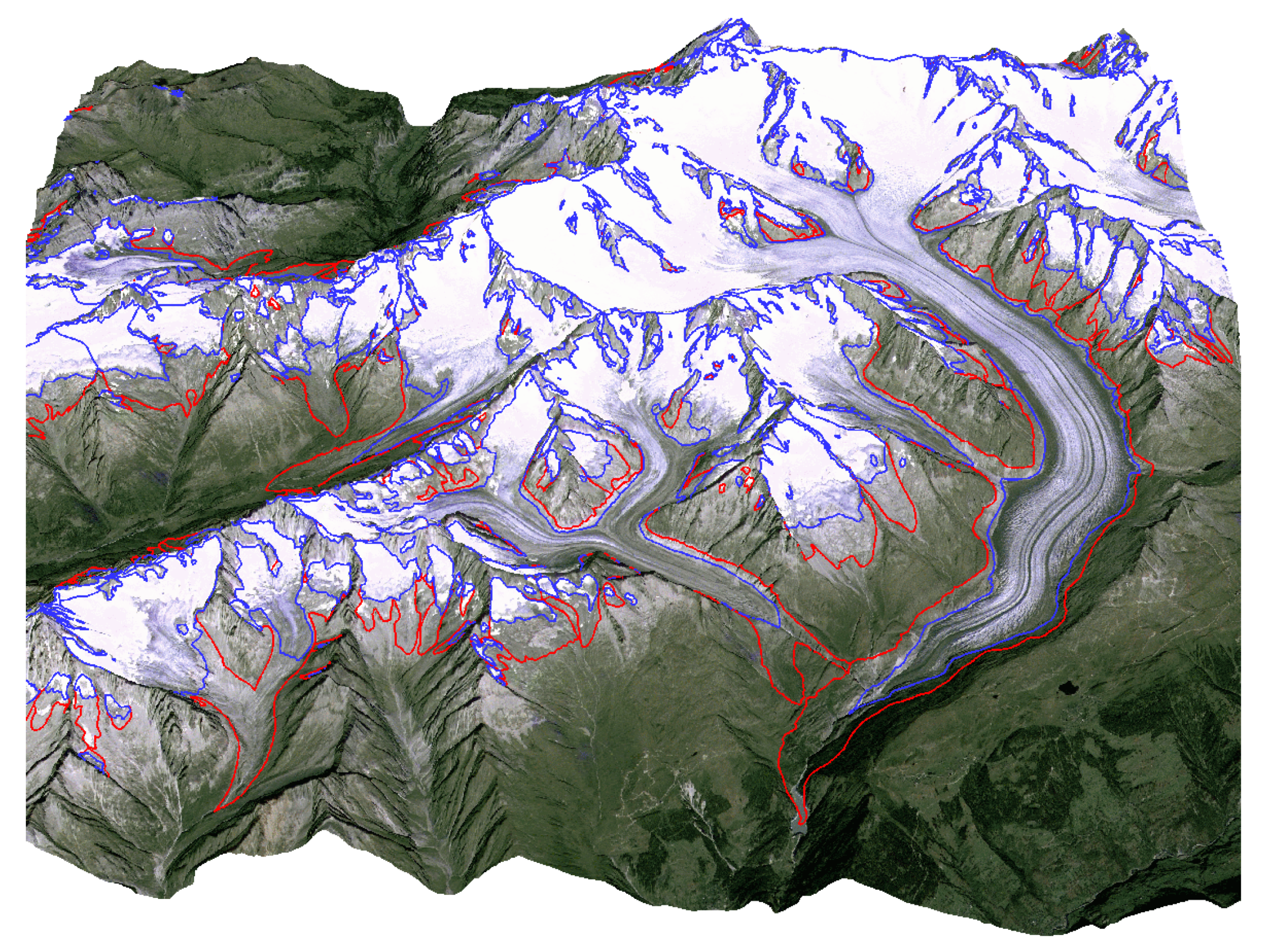
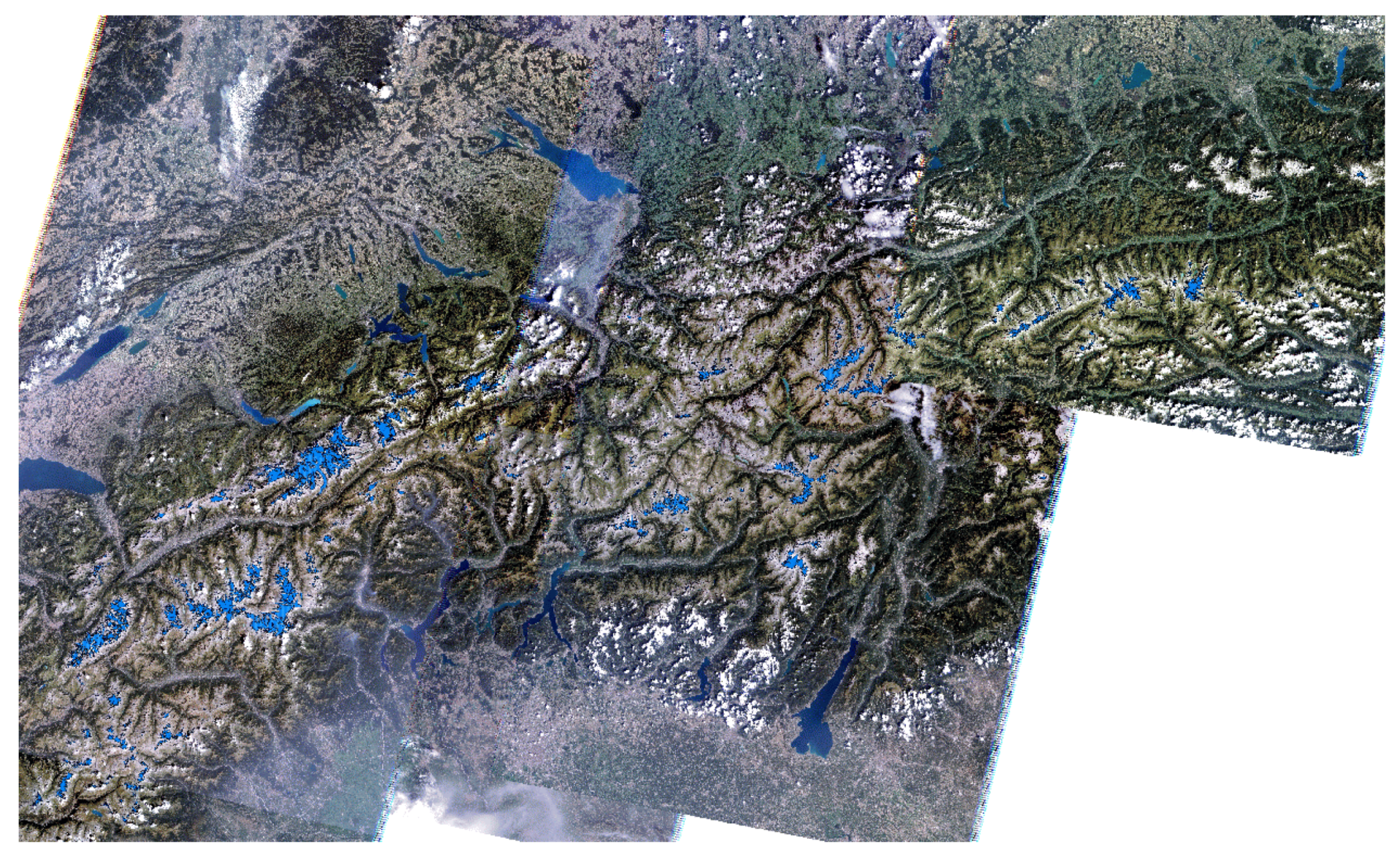
ECV Glaciers and Icecaps

Glaciers are widely recognized as unique demonstration objects for climate change impacts. Glacier inventories record basic data for the largest possible sample of glaciers at a given point in time. They provide an essential basis for numerous glaciological, hydrological, climatological and geomorphological investigations and should be repeated at regular intervals. These intervals should reflect typical response times of the glaciers in the region, i.e., a few decades (e.g., [31]). Inventories allow individual measurements (e.g., of area changes) to be extrapolated to an entire region and also to assess the representativness of the observations at a limited number of field sites for the entire sample. Typical examples are given for the size class specific calculation of glacier area changes for the entire Alps from a sample of Swiss glaciers [32] or the assessment of the representativeness of the glaciers with mass balance measurements for the mass loss of the entire Alps [33]. The compilation of a detailed global glacier inventory using satellite data is therefore one of the prime goals of GCOS [4]. The last inventory for the entire Alps was published about 20 years ago in the world glacier inventory (WGI) [34] that was compiled over a 30-year period (i.e., 1955–1985) from aerial photography and topographic maps. Though overall glacier changes in this period were comparably small, the 30-year compilation period is problematic for a sound change assessment as a comparable study in Norway has demonstrated [35].

With the opening of the Landsat archive at the United States Geological Survey (USGS) and the free availability of orthorectified satellite data it became possible to map glaciers over entire mountain ranges with well established semi-automated image segmentation techniques developed earlier [36]. These methods are based on the very low reflectance of snow and ice in the shortwave infrared (SWIR) part of the spectrum, and just require applying a threshold on a band ratio with Landsat bands 3 and 5 (i.e., red/SWIR) or equivalent bands on other sensors. This method has proven to provide robust and accurate results over a wide range of mapping conditions and is thus widely applied to generate glacier outlines in different parts of the world [37,38,39]. The mapping accuracy that can be reached depends on the region (for example, it is less good for debris-covered glaciers), the snow conditions (i.e., seasonal snow can hide the glacier perimeter) and on glacier size, but can be better than 5% of the total area [37,38,40]. The basic point is that the accuracy of a glacier outline does not depend on the applied algorithm in the main image processing stage, but on methodological interpretation in the post-processing stage (i.e., during manual editing). A sound error assessment in a classical sense is thus difficult to perform for this ECV. As topographic information (e.g., minimum and maximum elevation) for each glacier plays an essential role in a glacier inventory [41], the free availability of the digital elevation models (DEMs) from SRTM (90 m resolution) and the ASTER global DEM (GDEM) at 30 m resolution is a particular valuable asset. First comparisons have shown that both datasets are well suitable to derive glacier inventory parameters [42].

In a pilot study for the Swiss Alps and as a contribution to the Global Land Ice Measurements from Space (GLIMS) initiative, both data sources (satellite and DEM) were combined with modern geoinformatic techniques to derive an updated glacier inventory for the years 1998/99. For calculation of glacier specific size changes, also the inventories from 1850 and 1973 were digitized and combined with the same drainage divides [40]. As an example, the digital overlay of the outlines from 1850 and 1973 on the satellite image from 1998 is illustrated in Figure 4 with an oblique perspective view for the region around Great Aletsch Glacier. The strong size and volume loss over this period for the larger glaciers is well recognizable, but the area loss from 1973 to 1998/99 is less apparent at this scale. It was particular strong for the smaller glaciers that contribute more than 40% to the total area loss. Overall, an area loss of about 18% was calculated for this period. Thereby, a roughly 14% area loss took place after 1985 alone, which is about seven times higher than for the 1850–1973 period [32].

Figure 4. The region around Great Aletsch Glacier in a synthetic oblique perspective view created from a pan-sharpened satellite image (Landsat TM with IRS-1C) and glacier outlines from 1850 (red) and 1973 (blue) draped over a DEM. The region covered is 40 km by 41 km in size. DEM 25: Reproduced with permission by swisstopo (BA110151).

Figure 4. The region around Great Aletsch Glacier in a synthetic oblique perspective view created from a pan-sharpened satellite image (Landsat TM with IRS-1C) and glacier outlines from 1850 (red) and 1973 (blue) draped over a DEM. The region covered is 40 km by 41 km in size. DEM 25: Reproduced with permission by swisstopo (BA110151).

Within the framework of the ESA project GlobGlacier [43], the same glacier mapping approach was recently applied to the entire Alps using ten Landsat scenes acquired over a two-month period in the late summer of 2003 (Figure 5). In that year, an extraordinary heatwave caused nearly perfect glacier mapping conditions already in August (without seasonal snow outside of glaciers and high solar elevation, i.e., reduced shadow) in most regions of the Alps. A total of about 3,800 glaciers were mapped and topographic parameters were calculated from the SRTM DEM. This new inventory is more up-to-date than the WGI, but it is moreover derived with the same method from the same sensor over a very short period of time. This consistency has strong advantages for change assessment or spatio-temporal extrapolations, for example for the calculation of future glacier development in the Alps [44]. All glacier outlines and appended topographic information for each glacier will be available at no cost in a digital vector format (shape-file) from the GLIMS glacier database [45]. The total glacierized area mapped in this new inventory was ca. 2,050 km² which is about 30% less than in the WGI from the 1970s. Apart from the strong area loss from 1998 to 2003, it has to be considered that the acceleration of glacier decline is partly also due to the higher number of smaller glaciers in the entire sample (compared to Switzerland), which tend to have (in the mean) higher relative area changes than larger glaciers [32].

Though currently glacier inventory creation is mostly based on Landsat 5 (in operation since 1984) and 7, as well as the ASTER sensor onboard Terra, the mid-term prospects for glacier mapping is promising [46]. New satellites with optical sensors and sufficient spatial resolution like Sentinel-2 from ESA and LDCM (Landsat Data Continuity Mission) from NASA/USGS will be launched in a few years. They will provide a higher repetition rate and a continuation of the monitoring of this ECV. Additionally, more long-term projects like the recently started Glaciers_cci project as part of the ESA Climate Change Initiative [16] will contribute to a more complete global glacier inventory and help to establish an operational service for space-borne monitoring of the ECV ‘Glaciers and Icecaps’. Particular emphasize in this regard will be given to a couple of round-robin experiments with test sites from all over the world to improve the integrity and consistency of the datasets in the GLIMS glacier database.

Figure 5. The new glacier inventory for the entire Alps as obtained from ten Landsat TM scenes acquired in 2003. The background shows a mosaic of the scenes used in the inventory in natural colors and the light blue areas with black outlines depict the mapped glaciers. Image source: glovis.usgs.gov.

Figure 5. The new glacier inventory for the entire Alps as obtained from ten Landsat TM scenes acquired in 2003. The background shows a mosaic of the scenes used in the inventory in natural colors and the light blue areas with black outlines depict the mapped glaciers. Image source: glovis.usgs.gov.

4. Conclusions

Satellites now provide a vital means of obtaining observations of the climate system from a global perspective and comparing the state and development of ECVs in different parts of the globe [3]. This paper has described the important role and potential of satellites within the National Climate Observing System in Switzerland (GCOS Switzerland). The presented examples from the atmospheric domain (ECV ‘Cloud properties’) and the terrestrial domain (ECV ‘Glaciers and Icecaps’) have shown specific results of the use of satellite data for climate studies in Switzerland. The 10-year cloud cover climatology from MODIS from March 2000 until February 2010 gives an overall mean daytime cloud fraction of 64%, with large seasonal variations. In winter, the mean daytime monthly mean cloud fraction increases to about 71% while in summer, lower mean daytime monthly mean cloud fraction values of about 52% are measured. The comparison with ground-based synop observations shows a good agreement, with a mean difference of −2% ± 6% (i.e., synop values slightly higher than satellite-based values). The results will be further compared with time series derived from other satellite sensors (e.g., MODIS Aqua, Meteosat, NOAA AVHRR, MISR, (A)ATSR(2)). The glacier mapping methods developed for the Swiss glacier inventory are now applied worldwide to further complete the global glacier inventory as requested by GCOS and as a contribution to the GLIMS glacier database. The presented results from the Swiss Alps and the new Alpine-wide glacier inventory illustrate the massive loss in glacier area since the 1980s from about 2,900 km² in the WGI to 2,050 km² in 2003.

In the future, an adequate and periodical reprocessing of the long-term datasets is essential to provide consistent climate data records for regional applications. The frequency of the reprocessing will strongly depend on the ECV under consideration, on the availability of the respective satellite data, and the required efforts. Glacier mapping, for example, requires both manual editing of the outlines (e.g., for debris-covered regions) and expert knowledge to achieve an acceptable accuracy. This will result in longer time intervals for a complete updated dataset than for other ECVs that can be reprocessed by a fully automated algorithm. Initiatives, such as the Global Space-based Inter-Calibration System (GSICS) [47], play an important role in supporting the generation of long-term data records from satellite observations for climate analysis. In this respect, it is also important to stress the necessity of a thorough assessment of the errors for the different satellite-based products. Furthermore, the continuity of Earth Observation programs of climate relevant sensors is vital to guarantee homogeneous measurements of sufficient length. In Switzerland, archived datasets and existing algorithms developed for near real-time use over Switzerland represent an interesting potential for future climate studies. In addition, the high quality ground-based observations of various ECVs have a great potential for extensive calibration and validation studies over Switzerland (e.g., soundings, ground-based remote sensing). The same applies for the long tradition in field observations and methodical developments for glacier monitoring (e.g., [31]). Switzerland, with its many unique observation systems and climate records, can thereby help to further advance the integration of satellite data into comprehensive climate data records. The capabilities of existing and future observing systems will also be an important factor in the development of the Global Framework for Climate Services (GFCS) as decided at the World Climate Conference 3 (WCC-3) in 2009 [48]. The Swiss GCOS Office will continue to foster the generation of satellite-based datasets of ECVs for the area of Switzerland by various institutions and their combination with long-term in situ measurements to generate integrated high-quality climate data products within GCOS Switzerland.

References

1. The Second Report on the Adequacy of the Global Observing Systems for Climate in Support of the UNFCCC; WMO TD 1143; WMO GCOS-82; WMO GCOS: Geneva, Switzerland, 2003; p. 81.
2. Implementation Plan for the Global Observing System for Climate in Support of the UNFCCC; WMO TD 1219; WMO GCOS-92; WMO GCOS: Geneva, Switzerland, 2004; p. 136.
3. Implementation Plan for the Global Observing System for Climate in Support of the UNFCCC (2010 Update); WMO TD 1523; WMO GCOS-138; WMO GCOS: Geneva, Switzerland, 2010; p. 180.
4. Systematic Observation Requirements for Satellite-based Products for Climate; WMO TD 1338; WMO GCOS-107; WMO GCOS: Geneva, Switzerland, 2006; p. 90.
5. CEOS Satellite Observation of the Climate System: The Committee on Earth Observation Satellites (CEOS) Response to the Global Climate Observing System (GCOS) Implementation Plan (IP). 2006, p. 54. Available online: http://www.ceos.org/images/PDFs/CEOSResponse_1010A.pdf (accessed on 8 April 2011).
6. CEOS Coordinated Response from Space Agencies Involved in Global Observations to the Needs Expressed in the Global Climate Observing System (GCOS) Implementation Plan. Update on Climate Actions. 2008, p. 43. Available online: http://unfccc.int/resource/docs/2008/sbsta/eng/misc11.pdf (accessed on 8 April 2011).
7. CEOS 2010 Progress Report: Coordinated Response from Parties that Support Space Agencies Involved in Global Observations to the Needs Expressed in the Global Climate Observing System (GCOS) Implementation Plan of 2004; 2010; p. 111. Available online: http://www.ceos.org/images/CEOS-UNFCCC-2010.pdf (accessed on 8 April 2011).
8. Seiz, G.; Foppa, N. National Climate Observing System (GCOS Switzerland). Adv. Sci. Res. 2011. accepted. [Google Scholar] [CrossRef]
9. Seiz, G.; Foppa, N. National Climate Observing System (GCOS Switzerland). Publication of MeteoSwiss and ProClim. 2007, p. 92. Available online: http://www.gcos.ch (accessed on 8 April 2011).
10. Seiz, G.; Foppa, N.; Asch, A.; De Ruyter de Wildt, M. Snow Cover Climatology from Meteosat-8. In Proceedings of the Joint EUMETSAT Meteorological Satellite Conference and the 15th Satellite Meteorology & Oceanography Conference of the American Meteorological Society, Amsterdam, The Netherlands, 24–28 September 2007; p. 50.
11. Foppa, N.; Walterspiel, J.; Asch, A.; Seiz, G. Satellite-Based Climate Products for Alpine Studies within the Swiss GCOS Activities. In Proceedings of the EUMETSAT Meteorological Satellite Conference, Darmstadt, Germany, 8–12 September 2008; p. 52.
12. Seiz, G.; Foppa, N.; Walterspiel, J. Use of Satellite-Based Products within the National Climate Observing System (GCOS Switzerland). In Proceedings of the EUMETSAT Meteorological Satellite Conference, Bath, UK, 21–25 September 2009; p. 55.
13. Seiz, G.; Foppa, N. GCOS Switzerland. Progress Report 2008; Submission of Switzerland to the UNFCCC. 2008, p. 47. Available online: http://www.gcos.ch (accessed on 8 April 2011).
14. Dürr, B.; Zelenka, A. Deriving surface global irradiance over the Alpine region from METEOSAT Second Generation data by supplementing the HELIOSAT method. Int. J. Remote Sens. 2009, 30. [Google Scholar] [CrossRef]
15. Schulz, J.; Thomas, W.; Müller, R.; Behr, H.-D.; Caprion, D.; Deneke, H.; Dewitte, S.; Dürr, B.; Fuchs, P.; Gratzki, A.; Hollmann, R.; Karlsson, K.-G.; Manninen, T.; Reuter, M.; Riihelä, A.; Roebeling, R.; Selbach, N.; Tetzlaff, A.; Wolters, E.; Zelenka, A.; Werscheck, M. Operational climate monitoring from space: The EUMETSAT satellite application facility on climate monitoring (CM-SAF). Atmos. Chem. Phys. 2009, 9, 1687–1709. [Google Scholar] [CrossRef]
16. Plummer, S. The ESA Climate Change Initiative: Description; EOP-SEP/TN/0030-09/SP; Issue 1 Revision 0; ESA: Frascati, Italy, 2009; Available online: http://earth.eo.esa.int/workshops/esa_cci/ESA_CCI_Description.pdf (accessed on 8 April 2011).
17. Schiffer, R.A.; Rossow, W.B. The International Satellite Cloud Climatology Project (ISCCP): The first project of the World Climate Research Programme. Bull. Amer. Meteorol. Soc. 1983, 64, 779–784. [Google Scholar]
18. Rossow, W.B.; Duenas, E. The International Satellite Cloud Climatology Project (ISCCP) web site: An online resource for research. Bull. Amer. Meteorol. Soc. 2004, 85, 167–172. [Google Scholar] [CrossRef]
19. PATMOS-x Pathfinder Atmospheres–Extended; Cooperative Institute for Meteorological Satellite Studies, SSEC, UW-Madison: Madison, WI, USA, 2011; Available online: http://cimss.ssec.wisc.edu/patmosx/ (accessed on 8 April 2011).
20. Meerkötter, R.; Koenig, C.; Bissolli, P.; Gesell, G.; Mannstein, H. A 14-year European cloud climatology from NOAA/AVHRR data in comparison to surface observations. Geophys. Res. Lett. 2004, 31, L15103. [Google Scholar] [CrossRef]
21. King, M.D.; Menzel, W.P.; Kaufman, Y.I.; Tanré, D.; Gao, B.C.; Platnick, S.; Ackerman, S.A.; Remer, L.A.; Pincus, R.; Hubanks, P.A. Cloud and aerosol properties, precipitable water, and profiles of temperature and water vapor from MODIS. IEEE Trans. Geosci. Remote Sens. 2003, 41, 442–458. [Google Scholar] [CrossRef]
22. Platnick, S.; King, M.D.; Ackerman, S.A.; Menzel, W.P.; Baum, B.A.; Riédi, J.C.; Frey, R.A. The MODIS cloud products: Algorithms and examples from terra. IEEE Trans. Geosci. Remote Sens. 2003, 41, 459–473. [Google Scholar] [CrossRef]
23. Ackerman, S.; Frey, R.; Strabala, K.; Liu, Y.; Gumley, L.; Baum, B.; Menzel, P. Discriminating Clear-Sky from Cloud with MODIS. Algorithm Theoretical Basis Document (MOD35); Version 6.0; NASA: Greenbelt, MD, USA, 2010. Available online: http://modis-atmos.gsfc.nasa.gov/_docs/MOD35_ATBD_Collection6.pdf (accessed on 8 April 2011).
24. Hubanks, P.A.; King, M.D.; Platnick, S.A.; Pincus, R.A. MODIS Algorithm Theoretical Basis Document No. ATBD-MOD-30 for Level-3 Global Gridded Atmosphere Products (08_D3, 08_E3, 08_M3); MODIS Atmosphere L3 Gridded Product Algorithm Theoretical Basis Document; NASA: Greenbelt, MD, USA, 2008. Available online: http://modis-atmos.gsfc.nasa.gov/_docs/L3_ATBD_2008_12_04.pdf (accessed on 8 April 2011).
25. Kotarba, A.Z. A comparison of MODIS-derived cloud amount with visual surface observations. Atmos. Res. 2009, 92, 522–530. [Google Scholar] [CrossRef]
26. Oesch, D.C.; Jaquet, J.-M.; Hauser, A.; Wunderle, S. Lake surface water temperature retrieval using advanced very high resolution radiometer and Moderate Resolution Imaging Spectroradiometer data: Validation and feasibility study. J. Geophys. Res. 2005, 110, C12014. [Google Scholar] [CrossRef]
27. Foppa, N.; Hauser, A.; Oesch, D.; Wunderle, S.; Meister, R. Validation of operational AVHRR sub-pixel snow retrievals over the European Alps based on ASTER data. Int. J. Remote Sens. 2007, 28, 4841–4865. [Google Scholar] [CrossRef]
28. Huesler, F.; Wunderle, S.; Neuhaus, C. Towards a 25-year Snow Cover Time Series over the European Alps Derived from AVHRR Satellite Data. In Proceedings of the Extended Abstracts of the Conference Global Change and the World’s Mountains, Perth, UK, 26–30 September 2010.
29. Jolly, W.M.; Dobbertin, M.; Zimmermann, N.E. Divergent vegetation growth responses to the 2003 heat wave in the Swiss Alps. Geophys. Res. Lett. 2005, 32, L18409. [Google Scholar] [CrossRef]
30. Stöckli, R.; Vidale, P.L. European plant phenology and climate as seen in a 20 year AVHRR land-surface parameter dataset. Int. J. Remote Sens. 2004, 25, 3303–3330. [Google Scholar]
31. Haeberli, W. Glaciers and ice caps: Historical background and strategies of world-wide monitoring. In Mass Balance of the Cryosphere; Bamber, J.L., Payne, A.J., Eds.; Cambridge University Press: Cambridge, UK, 2004; pp. 559–578. [Google Scholar]
32. Paul, F.; Kääb, A.; Maisch, M.; Kellenberger, T.W.; Haeberli, W. Rapid disintegration of Alpine glaciers observed with satellite data. Geophys. Res. Lett. 2004, 31, L21402. [Google Scholar] [CrossRef]
33. Paul, F.; Haeberli, W. Spatial variability of glacier elevation changes in the Swiss Alps obtained from two digital elevation models. Geophys. Res. Lett. 2008, 35, L21502. [Google Scholar] [CrossRef]
34. Haeberli, W.; Bösch, H.; Scherler, K.; Østrem, G.; Wallén, C.C. WGMS World Glacier Inventory—Status 1988; IAHS (ICSI)/UNEP/UNESCO, World Glacier Monitoring Service: Zurich, Switzerland, 1989; p. 458. [Google Scholar]
35. Andreassen, L.M.; Paul, F.; Kääb, A.; Hausberg, J.E. Landsat-derived glacier inventory for Jotunheimen, Norway, and deduced glacier changes since the 1930s. The Cryosphere 2008, 2, 131–145. [Google Scholar] [CrossRef] [Green Version]
36. Paul, F.; Kääb, A.; Maisch, M.; Kellenberger, T.W.; Haeberli, W. The new remote-sensing-derived Swiss glacier inventory: I. Methods. Ann. Glaciol. 2002, 34, 355–361. [Google Scholar] [CrossRef] [Green Version]
37. Bolch, T.; Menounos, B.; Wheate, R. Landsat-based glacier inventory of western Canada, 1985–2005. Remote Sens. Environ. 2010, 114, 127–137. [Google Scholar] [CrossRef]
38. Paul, F.; Andreassen, L.M. A new glacier inventory for the Svartisen region, Norway, from Landsat ETM+ data: Challenges and change assessment. J. Glaciol. 2009, 55, 607–618. [Google Scholar] [CrossRef] [Green Version]
39. Albert, T. Evaluation of remote sensing techniques for ice-area classification applied to the tropical Quelccaya Ice Cap, Peru. Polar Geogr. 2002, 26, 210–226. [Google Scholar] [CrossRef]
40. Paul, F. The New Swiss Glacier Inventory 2000—Application of Remote Sensing and GIS. Ph.D. Thesis, Department of Geography, University of Zurich, Zurich, Switzerland, 2007; p. 210. [Google Scholar]
41. Paul, F.; Barry, R.; Cogley, G.; Frey, H.; Haeberli, W.; Ohmura, A.; Ommanney, S.; Raup, R.; Rivera, A.; Zemp, M. Recommendations for the compilation of glacier inventory data from digital sources. Ann. Glaciol. 2009, 50, 119–126. [Google Scholar] [CrossRef] [Green Version]
42. Frey, H.; Paul, F. On the suitability of the SRTM DEM and ASTER GDEM for the compilation of topographic parameters in glacier inventories. Int. J Appl. Earth Obs. Geoinf. 2011. submitted. [Google Scholar] [CrossRef]
43. Paul, F.; Kääb, A.; Rott, H.; Shepherd, A.; Strozzi, T.; Volden, E. GlobGlacier: Mapping the world’s glaciers and ice caps from space. EARSeL eProceedings 2009, 8, 11–25. [Google Scholar]
44. Kotlarski, S.; Jacob, D.; Podzun, R.; Paul, F. Representing glaciers in a regional climate model. Clim. Dynam. 2010, 34, 27–46. [Google Scholar] [CrossRef] [Green Version]
45. Raup, B.H.; Racoviteanu, A.; Khalsa, S.J.S.; Helm, C.; Armstrong, R.; Arnaud, Y. The GLIMS geospatial glacier database: A new tool for studying glacier change. Global Planet. Change 2007, 56, 101–110. [Google Scholar] [CrossRef]
46. Paul, F. Towards a global glacier inventory from satellite data. Geograph. Helv. 2010, 65, 103–112. [Google Scholar] [CrossRef]
47. WMO Implementation Plan for a Global Space-Based Inter-Calibration System GSICS, Version 1, CGMS 34 (11/06); April 2006. Available online: http://www.wmo.int/pages/prog/sat/GSICS/documents/GSICS_IP.pdf (accessed on 8 April 2011).
48. Karl, T.R.; Diamond, H.J.; Bojinski, S.; Butler, J.H.; Dolman, H.; Haeberli, W.; Harrison, D.E.; Nyong, A.; Rösner, S.; Seiz, G.; Trenberth, K.; Westermeyer, W.; Zillman, J. Observation needs for climate information, prediction and application: Capabilities of existing and future observing systems. Procedia Environ. Sci. 2010, 1, 192–205. [Google Scholar] [CrossRef]