1. Introduction
Digital Elevation Model (DEM) is one of the important components of the digital spatial data environment and its applications. In Earth Sciences, the elevation refers to the height from the Mean Sea Level (MSL) to the bald Earth surface. The digital representation of such measurements is called a DEM. An elevation model can be represented as regular or irregular point clouds formed into a mathematical model. In order to represent the continuous Earth surface these point clouds should form into the shape of the surface. There are various methods for doing this and Triangulated Irregular Network (TIN) is one of the most popular methods [
1].
Commencing from the early 1300s with Jacob Staff and Compass until today, the generation of elevation models have evolved from hand drawn or field drawn (With Plane Table Alidade in late 1800s) topo and planimetric maps, to digital representation as DEMs. Considering all the aspects involved such as costs, ease of use, rate of capture, applicability, accuracy, and repeatability until the final product is achieved, use of the Light Detection and Ranging (LIDAR), Laser Terrestrial Scanning (LTS) and satellite remote sensing for data capture, developing automated methods to obtain DEMs would be the better approach.
Due to the advancement of High Resolution Satellite Images (HRSI) with stereo capabilities, digital photogrammetric method for generating DEMs and Orthoimages are becoming more popular. At present, the major issues of DEM generation with respect to the consistency, availability, cost, degree of resolution and coverage have been overcome while some issues are still remaining. One of the major issues still remaining is the generation of DEM and not a DSM in areas where the terrain is covered by various objects. Presently available digital data sources observe top of the surface where the energy is reflecting and producing a combination of DSM and DEM point clouds by automated image matching techniques that are already well documented. Due to this reason, satellite data provides a DSM not a DEM. In order to get a DEM, the DSM needs to project onto bald terrain.
Currently, filtering techniques are the most popular methods used for converting a DSM to DEM. In most cases, the off terrain point clouds are filtered out and the created hollow areas are interpolated using surrounding DEM points. The main drawback of this method is the waste of valuable information and large area of uncontrolled terrain points. While interpolating the space to predict the DEM that will be unpredictable without information, there were many other issues in filtering of DSM point clouds in these off terrain areas that were stated by several authors as described below.
The filtering techniques used to remove the off terrain point clouds will also remove the bald terrain matched points when the area is not flat [
2]. The filtering is not possible with simple filtering techniques [
3]. The particular filtering method cannot be applied to other different areas as it depends on configurations of terrain with manmade and natural objects [
2]. It is difficult to find the correct trade-off between removing low vegetation and preserving small height jumps in the terrain [
4]. The filtering of off-terrain points is critical and may result in a large data void [
5]. The NGATE (
Next-
Generation
Automatic
Terrain
Extraction) software product that was released in 2008 by BAE Systems claims that the resultant photogrammetrically derived DTMs are first-rate, but it has to be considered together with rather modest interactive editing using the ITE (
Interactive
Terrain
Editing) module. Hence, it will not be a full complete automatic generation DTM method [
6]. Another presently available software, SCOP++, is designed for interpolation, management, application and visualization of digital terrain data, with special emphasis on accuracy. SCOP++ aims at high quality of interpolation and of all products derived from the model, and for processing huge amounts of DTM data [
7]. From this point of view, there are still many problems that have to be solved before generating DTM using presently available methods. The main problems of reducing DSM to DTM have to be solved and the most successful approaches should be identified. This is one of the key issues in DTM generation. As manual editing needs a lot of time, it is necessary to solve how to generate DTM using an automated method. In addition, due to the fact that presently available methods are purely based on geometrical considerations, the results are not realistic [
8].
However, the point clouds in off terrain areas that were generated by image matching are wasted due to the removal of these point clouds by presently available DEM generation methods. Further, in the hollow spaces obtained after removing the off terrain areas, it is difficult to predict any kind of distribution which follows the terrain pattern for interpolating.
The objective of this paper is to use these off terrain point clouds in a useful way to generate DEM especially in dense forest areas where no DEM points can be identified inside the space. In addition, generating DEM from DSM where the few points inside the space are available is also discussed. Attempt is made to use DEM and DSM points available in the perimeter of the hollow space and a few well distributed points inside the hollow space.
As it is difficult to predict the distribution of the topography in areas where no terrain points are available, a distribution free method as well as the ability to predict the patterns and trends of the given data has to be used to obtain the terrain points from sample data. There are several methods that do not make pre-assumption of the distribution, such as Artificial Neural Networks (ANN), Classification And Regression Trees (CART), Multivariate Adaptive Regression Splines (MARS), etc. It was intended to use available open source software so the algorithms can be edited or new algorithms can be developed and adopted as required. Hence, it was intended to develop and use the ANN algorithm for projecting the DSM data into DEM data.
Several artificial neural network models have been designed and used for different applications. Some of these models are Perceptron, Madaline, Avalanche, Back Propagation, Neocognition, Adaptive Resonance Theory (ART), Self-Organizing Map (SOM), Hopfield, and Counter Propagation [
9].
3. Methodology
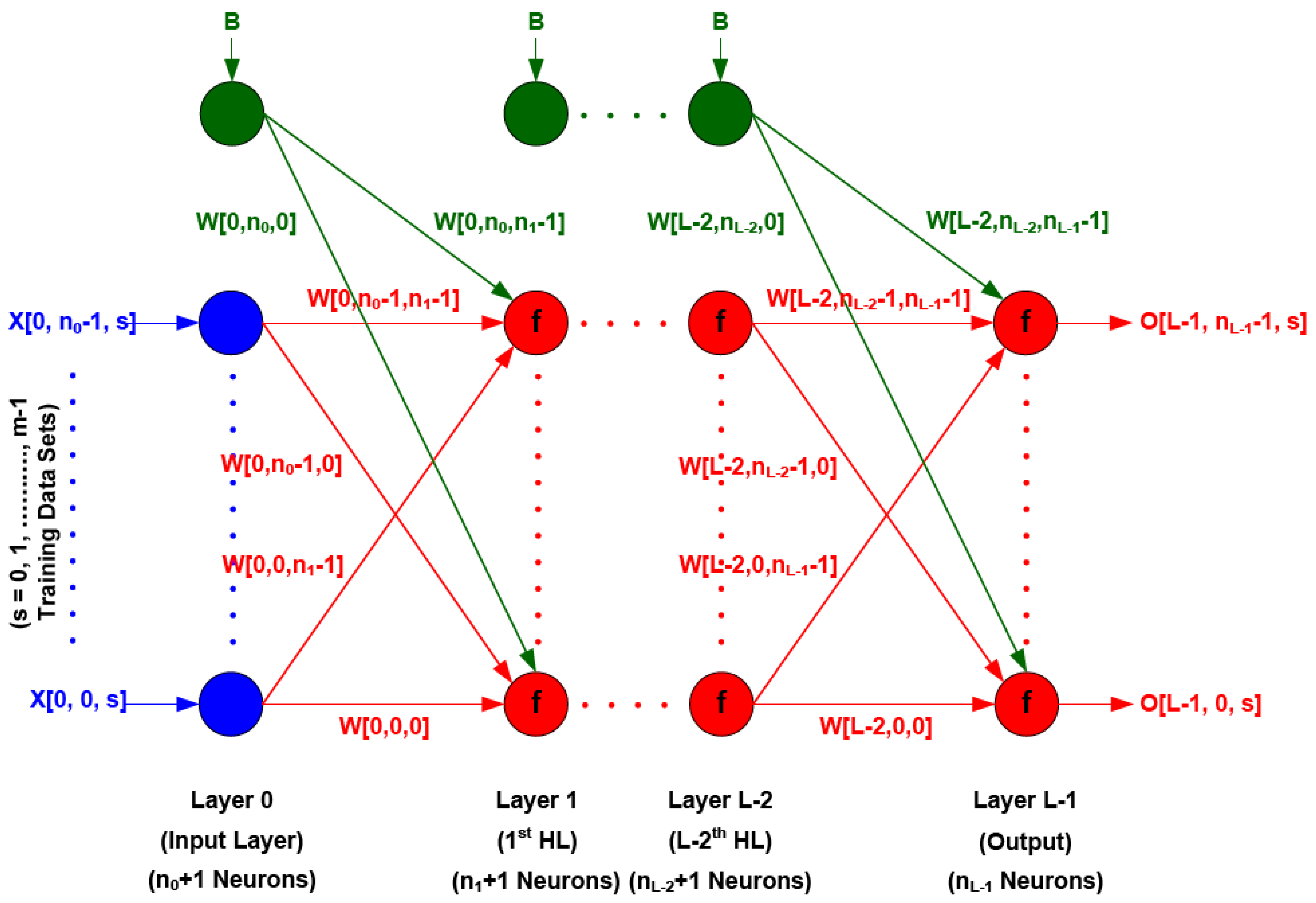
Multi-Layer Back Propagation (MLBP) network is still the most popular and widely used for pattern recognition and, until now, it has not been decided which kind of architecture is most suitable for the particular application. Hence, the different architectures should be investigated for a particular application. In this research, it is intended to use the MLBP supervised learning procedure as it is learning the requirement of the specific study. A general multi layer network is illustrated in
Figure 3 and the following calculation of errors at the output nodes refer to it. An iterative procedure is required to train the network as the network is nonlinearity; hence explicit a solution for the weights is impossible [
10].
Input layer and input data are depicted in blue, hidden layers and output layers with weights and activation functions are depicted in red and bias neuron set to +1 (B = 1) to make the connection weights as a threshold for that neuron, or set to zero (B = 0) when the fixed thresholds were used, are depicted in green.
Figure 3.
Architecture of multilayer back propagation artificial neural network.
Figure 3.
Architecture of multilayer back propagation artificial neural network.
Reference:
- B:
Bias Neuron
- W:
Weight
- L:
Number of Layers (Including Input and Output Layers)
- nL:
Number of neurons except the bias neuron in layer L
- X:
Input data
- O:
Output data
Referencing to the
Figure 3, the input (I) and output (O) of the bias neurons and mean squared error functions for batch and sequential processing are as follows.
where, r = 1,
2,..., L − 1.
It is well known that the neural network back propagation algorithm minimize the mean squared error function until the requirement is achieved.
If the desired output of k
th neuron is D[L − 1, k, s] for the s
th training sample, then the mean squared error function for the batch processing is E, given by,
where, m is the number of training samples.
For sequential training the mean squared error function at the training sample t is given by,
when the difference between the desired output and the network output at each output node is less than or equal to the given value (for sequential processing) or Root Mean Square Error (RMSE) as the overall error less than or equal to the given value (for batch processing), the network weights are adjusted by applying error correction (minimizing the most frequently used above error function) going backward in the network. In this iteration process, network is adjusting until the requirement is achieved.
This weight adjusting is based on a gradient descent method to minimize the above error cost function and it is a backward propagation of the network commencing from the output nodes until ending at the input nodes.
An application oriented ANN software was developed including the use of all the relevant parameters by using Microsoft Visual C++ 2008 programming language. It was facilitated for the use of planimetric coordinates and altitudes as text files of the DSMs as input, with relevant DEMs values to compare with the output height values. In addition, the facility to automatically stop the network training, when the given percentage of the sample DSM points is projected to DEM for given accuracy, was included because the ANN may not be trained for the whole data set. The use of trained ANN for any data sets was available in the software and for this purpose all relevant data files after being trained were stored automatically by creating a sub-directory.
As there is no appropriate architecture in ANN to use for the particular application, it was necessary to test out different architectures for this application. This is the critical point of ANN as many parameters are involved for differentiating the ANN architectures. Hence, it was checked initially with the previous researchers’ recommendations to establish the preliminary parameters of ANN such as number of hidden layers, number of neurons in hidden layers, and initial learning rate.
A neural network with two hidden layers can represent functions with any kind of shape and there is no theoretical reason to use more than two hidden layers [
11]. However, using more hidden layers was investigated for ANN, but proved too difficult to train and too time consuming. Hence, two hidden layers were used for this application.
Considering the number of neurons in hidden layers, using too few neurons will result in under fitting while using too many will result in over fitting. Over fitting can happen even when the training data is sufficient. Also using too many neurons can increase the time it takes to train the ANN [
5]. Any functional
mapping can be exactly represented by a three layer ANN with (2 m + 1) neurons in middle layers where m is the number of neurons at the input layer [
12], assuming that the input components are normalized to lie in the range [0,1]. Hence, it was intended to use seven neurons for each hidden layer when using altitude with its planimetric coordinates as input (three input neurons) while testing the other number arbitrarily by trial and error.
Small values were applied for initial learning rate to avoid oscillating the error. When using adaptive learning rate and momentum, no significant changes appeared. A momentum term was added also to reduce the time for convergence of the network and checked using different values of momentum by trial and error.
All other parameters, such as the use of thresholds for neurons whether fixed or weighted, the range of initial weights assignment, data normalizing procedure, use of activation function, and the processing methods whether the sequential or batch, were checked by comparing different approaches. Indeed, it was a time consuming process as there are so many combinations.
Finally, the following parameters were identified as suitable to train the ANN in this test area (T1) by investigating the different architectures with different parameters several times.
Two hidden layers [
11] with 7 neurons in each as number of input nodes were 3 for x, y, and z so the nodes for hidden layers is 7 [
12], 0.001 initial learning rate, 0.1 initial momentum, fixed thresholds for each hidden and output neurons and the value used to fire all neurons for any total input, sigmoidal data normalization, without adaptive learning rate and momentum, and [−1,1] initial range of weights were used for training the ANN. The input data and output desired data were normalized to the range of [−1,1] with sigmoidal transformation and so the Bipolar Sigmoid function was used as the activation function for all hidden and output neurons, where the output range of the function was also in the range of [−1,1].
Several investigations identified the sequential training method was most suitable for the application and was therefore used. Further, there are many advantages in using sequential training as it is often much faster, especially when the training set is redundant (contains many similar data points) and the noise in the gradient can help escape from local minima (which is a problem for gradient descent in nonlinear models) [
10].
The DSM altitude range of the selected training sample (Nine well distributed points) for T1 was 259.7 to 412.8 m and was 250.7 to 402.2 m for DEM. The ANN was trained with the Root Mean Square Error (RMSE) of 2.8 m with the mean error −0.3 for nine sample points by 3,017,521 iterations within 02 h 25 min 21 s.
This trained ANN was used to project the available 1 m resolution DSM data set of the T1 test area. To normalize and de-normalize the DSM and the projected DTM respectively, the same mean and standard deviation of the training DSM data sets were used [
13]. After projecting the whole DSM data set by using trained ANN, the accuracy was checked with the available corrected DEM data set and its RMSE was 1.3 m. After extraction of DSM data set within the same range of [min, max] and [mean−standard deviation, mean+standard deviation] of the trained DSM data, the RMSEs of these projected data obtained 1.4 m and 1.5 m respectively. This was done to check whether the trained ANN has the ability to project the data with the same range of data set used in its training phase.
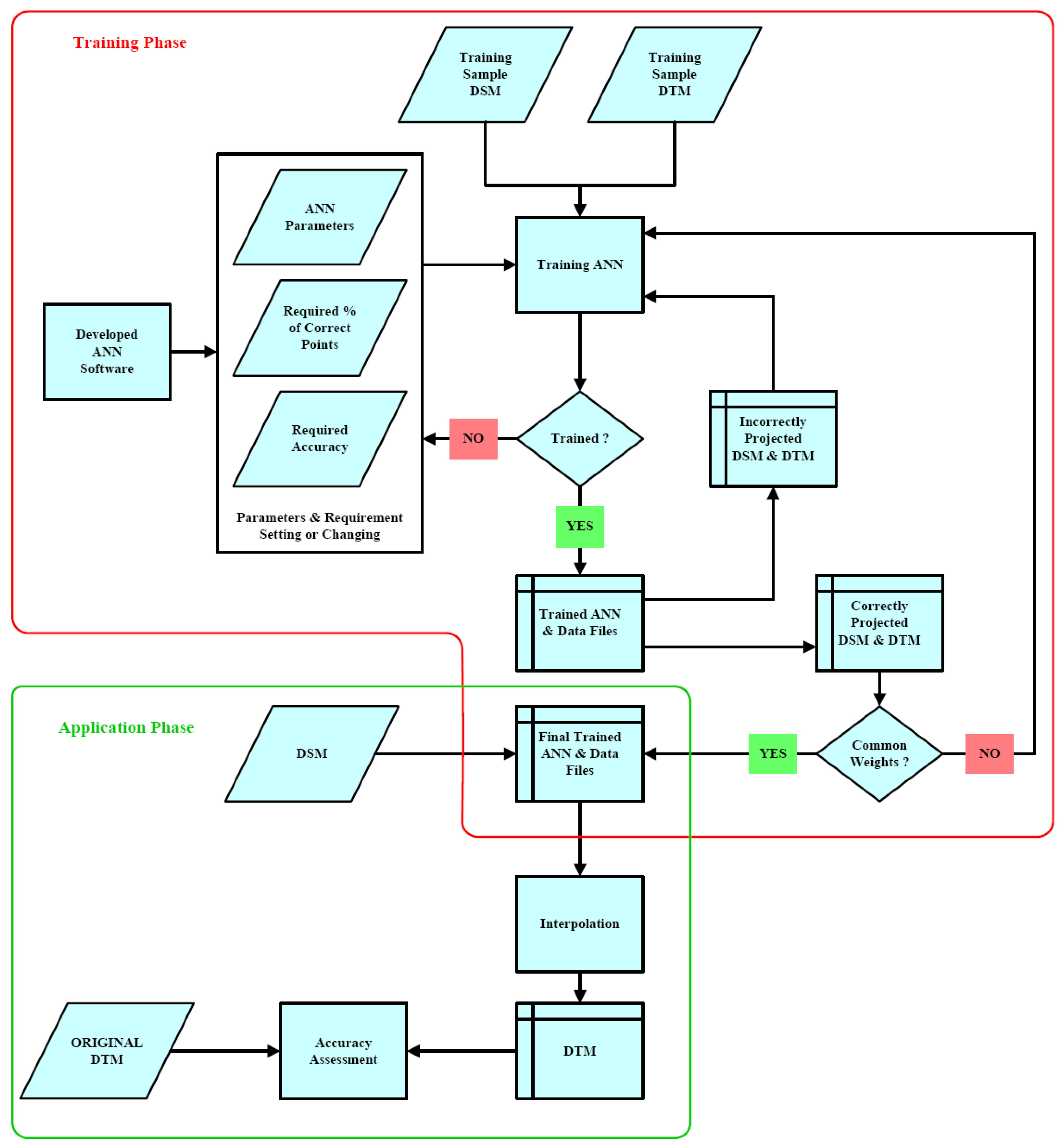
The different sets of ANN projected data were checked with the reference DEM data set and accuracies were assessed. The ANN projected DEM data sets were used to apply the different interpolation methods available in ArcGIS to obtain the DEMs for the whole T1 test area. In ArcGIS, there are several methods available for interpolation and we used Inverse Distance Weighed (IDW), Kriging, Natural Neighbor, Spline and Topo to Raster methods with their default parameters as it was not interesting to elaborate the interpolation methods, but the ability of ANN to project the DSM data into DEM. The schematic diagram of the procedure for DEM generation by ANN is illustrated in
Figure 4.
Figure 4.
Schematic diagram of the procedure for DTM generation by ANN.
Figure 4.
Schematic diagram of the procedure for DTM generation by ANN.
4. Results and Discussions
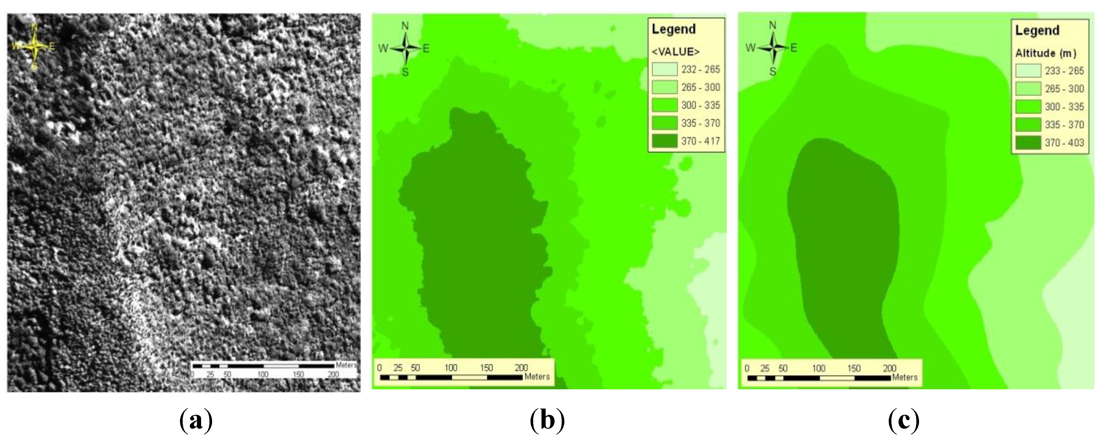
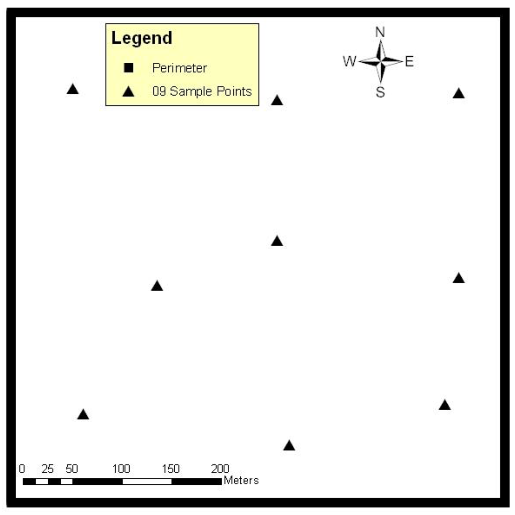
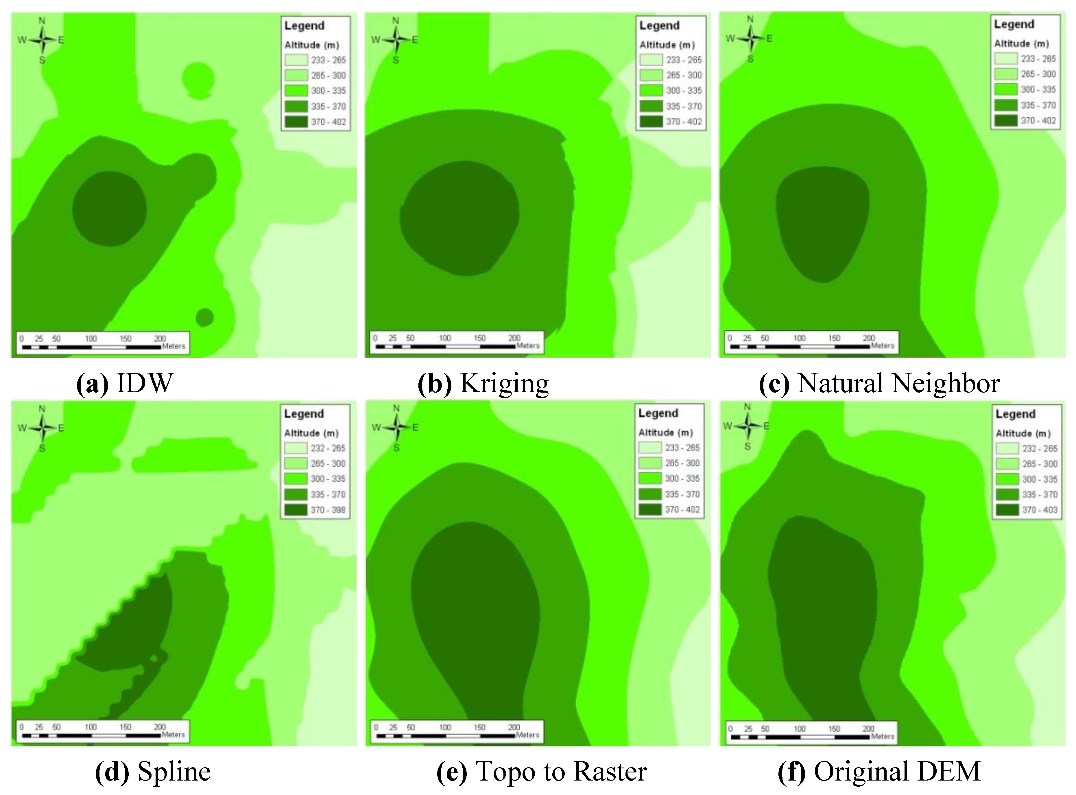
The accuracies of the DEM generation without using ANN, just interpolation with the available perimeter DEM data, obtained nine points for sample inside the T1 test site, and are given in
Table 1. The Inverse Distance Weighted (IDW), Kriging, Natural Neighbor, Splines, and Topo to Raster interpolations methods were used and the resulting DEMs are depicted in
Figure 5(a–e) with the reference DEM in
Figure 5(f). The interpolation methods such as Kriging and Natural Neighbor were used in ArcGIS giving slightly better results, but other interpolation methods such as Inverse Distance Weighted, Splines, and Topo to Raster techniques have given the worst results in accuracies of the DTM. The highest accuracy was obtained by Natural Neighbor interpolation for the combination of periphery and the well distributed nine points sample data sets. This was 5.5 m (
Table 1 and
Figure 5(c)).
Table 1.
Accuracies of interpolated DEM with perimeter and nine sample points of T1 test site.
Table 1.
Accuracies of interpolated DEM with perimeter and nine sample points of T1 test site.
| Interpolation Method | Mean (m) | RMSE wrt reference DEM (m) | Figure |
|---|
| IDW | 14.7 | 13.0 | 5(a) |
| Kriging | 8.1 | 9.9 | 5(b) |
| Natural Neighbor | 4.1 | 5.5 | 5(c) |
| Spline | 10.3 | 14.8 | 5(d) |
| Topo to Raster | −1.6 | 14.3 | 5(e) |
Figure 5.
Interpolated DEM with only perimeter and nine sample points of T1 test site.
Figure 5.
Interpolated DEM with only perimeter and nine sample points of T1 test site.
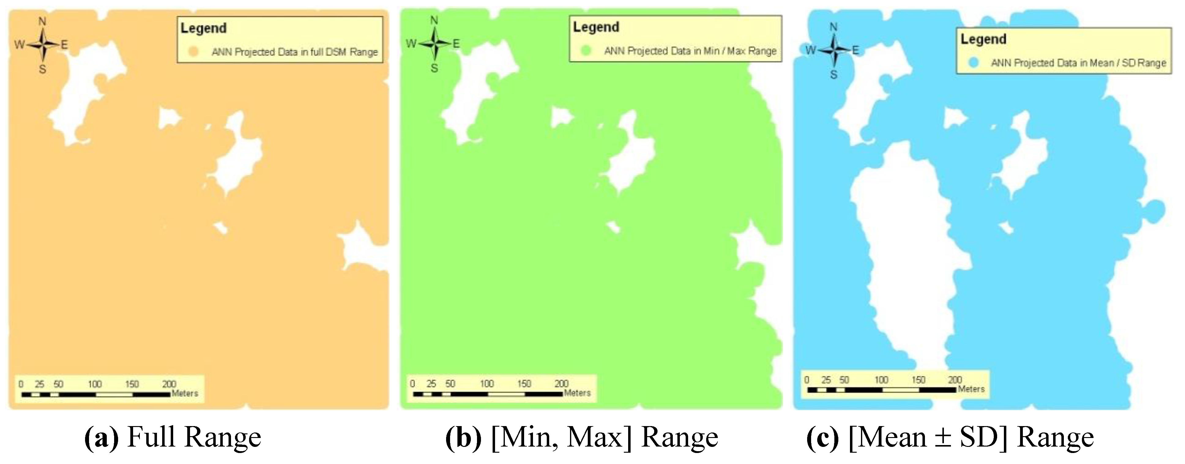
The nine sample points inside the area in T1 test site were trained by the ANN with the RMSE 2.891 m by 3,017,521 iterations within 02 h 25 min 21 s. To project DSM data to DEM, the DSM data was extracted to the [min, max] and [mean−SD, mean+SD] of the used DSM samples for training the ANN in addition to the projection of whole DSM data set. DSM data sets were projected to the DEM using the trained ANN. The relevant projected DEMs are given in
Figure 6(a–c). The accuracies of these projected DEMs are given in
Table 2 and they are 1.3 m, 1.4 m, and 1.5 m respectively. Further, the ANN projected DEM from the whole DSM was covered by the whole area, but the other data sets were not covered by the whole area (
Figure 6(a–c)).
All ANN projected DSM data ranges with the perimeter DEM data were used in all interpolation methods to obtain DEMs for the whole area. The accuracies of the different interpolated DEMs of the projected data sets for the [mean−SD, mean+SD] range DSM data set, and [min, max] range of DSM data set including the ANN projected DEM by whole DSM are given in
Table 3.
Table 2.
Accuracies of ANN projected DEM data for different DSM data ranges of the T1 test site.
Table 2.
Accuracies of ANN projected DEM data for different DSM data ranges of the T1 test site.
| DSM Data Range Used to ANN Projection by trained ANN | Mean (m) | RMSE of ANN Projected DTM wrt reference DEM (m) | Figure |
|---|
| Full Range (Whole DSM) | 0.6 | 1.3 | 6(a) |
| [min, max] = [259.640, 412.380] m range of ANN trained 9 points | 0.8 | 1.4 | 6(b) |
| Mean and SD = [280.431, 376.213] m range of ANN trained 9 points | 0.6 | 1.5 | 6(c) |
Figure 6.
ANN projected DEM data for different DSM data ranges of the T1 test site.
Figure 6.
ANN projected DEM data for different DSM data ranges of the T1 test site.
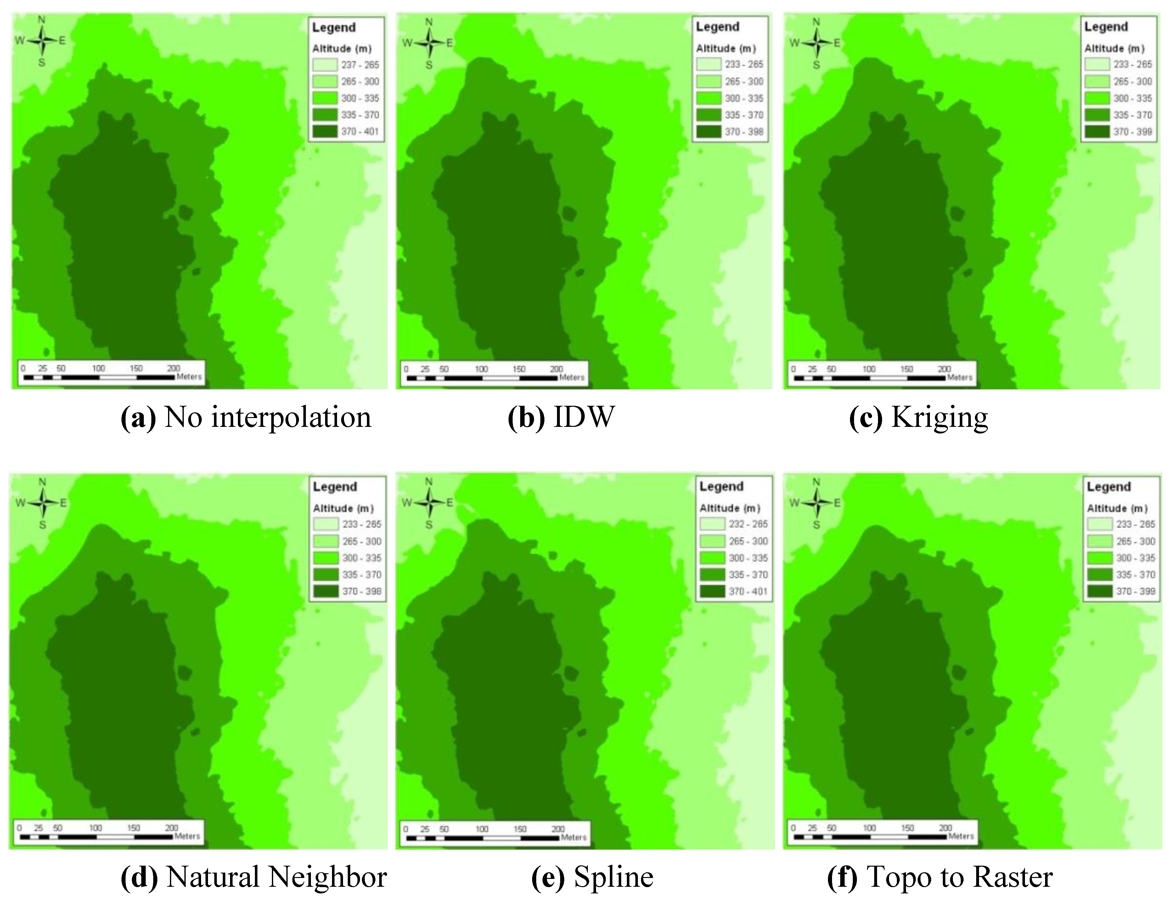
The sets of generated DEMs with different interpolation methods of the ANN projected [min, max] DSM data range with the perimeter DEM are given in
Figure 7(b–f), where the highest accuracies were obtained with the ANN projected DEM by whole DSM, as given in
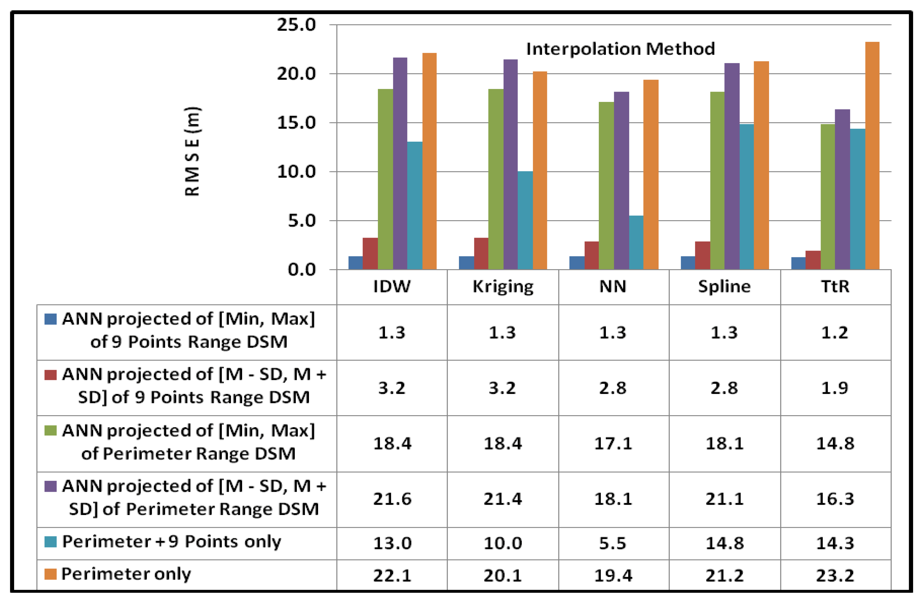
Figure 7(a). The comparison of accuracies of all finally generated DEMs was depicted as a graph in
Figure 8.
Table 3.
Final DEMs accuracies after interpolation of projected DEMs data with perimeter DEM.
Table 3.
Final DEMs accuracies after interpolation of projected DEMs data with perimeter DEM.
| Interpolation Method | Projected DSM Data Range | Mean (m) | RMSE of Final DEM wrt reference DEM (m) | Figure |
|---|
| No Interpolate | ANN Projected whole DSM | 0.6 | 1.3 | 7(a) |
| IDW | [min, max] | 0.7 | 1.3 | 7(b) |
| [M−SD, M+SD] | 2.4 | 3.2 | |
| Kriging | [min, max] | 0.8 | 1.3 | 7(c) |
| [M−SD, M+SD] | 2.4 | 3.1 | |
| Natural Neighbor | [min, max] | 8 | 1.3 | 7(d) |
| [M−SD, M+SD] | 2.3 | 2.8 | |
| Spline | [min, max] | 0.8 | 1.3 | 7(e) |
| [M−SD, M+SD] | 2.1 | 2.8 | |
| Topo to Raster | [min, max] | 0.6 | 1.2 | 7(f) |
| [M−SD, M+SD] | 1.7 | 1.9 | |
Figure 7.
Interpolation of ANN projected DEMs of [min, max] DSMs range with the perimeter DEM.
Figure 7.
Interpolation of ANN projected DEMs of [min, max] DSMs range with the perimeter DEM.
Figure 8.
Accuracy comparison of finally generated different DEMs.
Figure 8.
Accuracy comparison of finally generated different DEMs.
The highest accuracy was obtained using the Topo to Raster interpolation method with the combination of ANN projected data of [min, max] extracted DSM and the periphery of the area, and it was 1.2 m, but the others also have close accuracies such as 1.3 m. Excepting the use of [mean−SD, mean+SD] DSM data range used for ANN projection, all other data sets and interpolation methods gave similar accuracies from a statistical point of view. All of them were less than or equal to 1.3 m accuracy.
Due to the missing DSM data in the tails of the distribution when the range was [mean−SD, mean+SD] for ANN projection, many gaps still remained and hence the accuracies were reduced when interpolating.
The trained ANN of the T1 test site was used to project the DSMs of T2 to T5 test sites and the accuracies were assessed. These accuracies were less than the accuracies obtained for T1 test site and hence the ANN was trained with the samples obtained from the respective test sites T2 to T5 and then the DSMs to DEMs were projected and interpolated. It was seen that the accuracies obtained were similar as the accuracies obtained for the T1 test sites. However, it can be seen that if the areas of the test sites were getting larger, the accuracies were reduced and if the areas of the test sites were getting smaller the accuracies were increased.


