Article

Analysis of Vegetation Behavior in a North African Semi-Arid Region, Using SPOT-VEGETATION NDVI Data

1
CESBIO (CNRS, IRD, CNES, UPS), 18 Avenue Edouard Belin, bpi 2801, 31401 Toulouse cedex 9, France
2
INAT, 43, Avenue Charles Nicolle 1082, Tunis-Mahrajène, Tunisia
*
Author to whom correspondence should be addressed.
Remote Sens. 2011, 3(12), 2568-2590; https://0-doi-org.brum.beds.ac.uk/10.3390/rs3122568
Submission received: 13 September 2011 / Revised: 14 November 2011 / Accepted: 14 November 2011 / Published: 29 November 2011

Abstract

:
The analysis of vegetation dynamics is essential in semi-arid regions, in particular because of the frequent occurrence of long periods of drought. In this paper, multi-temporal series of the Normalized Difference of Vegetation Index (NDVI), derived from SPOT-VEGETATION satellite data between September 1998 and June 2010, were used to analyze the vegetation dynamics over the semi-arid central region of Tunisia. A study of the persistence of three types of vegetation (pastures, annual agriculture and olive trees) is proposed using fractal analysis, in order to gain insight into the stability/instability of vegetation dynamics. In order to estimate the state of vegetation cover stress, we propose evaluating the properties of an index referred to as the Vegetation Anomaly Index (VAI). A positive VAI indicates high vegetation dynamics, whereas a negative VAI indicates the presence of vegetation stress. The VAI is tested for the above three types of vegetation, during the study period from 1998 to 2010, and is compared with other drought indices. The VAI is found to be strongly correlated with precipitation.

1. Introduction

Vegetation cover, which affects different processes, in particular the water cycle, absorption and reemission of solar radiation, carbon cycling, and latent and sensible heat fluxes, plays a key role in land surface processes [1,2]. Any change to the vegetation cover can thus have a strong influence on local, regional and even global scales. In the case of arid and semi-arid areas in particular, because of frequent drought events, it is essential to have an accurate description of the vegetation cover and its variation over time. In recent years, large-scale intensive droughts, affecting large areas, have been observed on all continents, and the high associated economic and social costs have drawn increasing attention to the importance of droughts [3]. It is important to note that a drought corresponds to a period of temporary dryness, in contrast to the permanent dryness found in arid areas. Drought is associated with below-normal precipitation, which lasts for a period of months or even years.
Several studies have been carried out in an effort to improve the understanding of droughts. A number of different indices have been developed to quantify drought, each with its own strengths and weaknesses. They can be classified according to the following three types:
-
Drought indices based on precipitation measurements (e.g., Palmer Drought Severity Index (PDSI; [4]), rainfall anomaly index (RAI; [5]), deciles [6], crop moisture index (CMI; [7]), Bhalme and Mooly drought index (BMDI; [8]), surface water supply index (SWSI; [9]), national rainfall index (NRI; [10]), standardized precipitation index (SPI; [11,12]), and reclamation drought index (RDI; [13]). The PDSI is one of the most prominent indices used for meteorological drought, and can quantify long-term changes in aridity over global land masses [14]. It incorporates prior precipitation, moisture supply, and moisture demand into a hydrological accounting system. A multi-scalar drought index based on precipitation and evapotranspiration, called the Standard Precipitation and Evapotranspiration Index, has also been proposed by Vicento Serrano et al. (SPEI) [15].
-
Drought indices based on soil moisture estimations (e.g., soil moisture drought index (SMDI; [16])
-
Drought indices based on optical satellite observations. In recent decades, optical remote sensing has demonstrated its strong potential for the monitoring of vegetation dynamics and its variations over time, mainly because it provides a wide spatial coverage and its internal data sets are consistent. In particular, the Normalized Difference Vegetation Index (NDVI) is an equation of contrasting reflectance between the red and near-infrared regions of a surface spectrum [17]. This equation is a readily usable quantity that can be related to the green vegetation cover or vegetation abundance, and is expressed by: NDVI = (RNIR − RRED)/(RNIR + RRED), where RNIR is the near-infrared (NIR) reflectance and RRED is the red reflectance. This index is sensitive to the presence of green vegetation [18]. It has been used for several regional and global applications, in studies concerning the distribution and potential photosynthetic activity of vegetation [19,20,21,22,23,24]. Due to its formulation, it robustly describes green vegetation in spite of varying atmospheric conditions in the red and NIR bands [25,26]. This index is also considered to be a reliable indicator for land cover variations [27,28,29,30], since its temporal variations are strongly related to changes in the earth’s surface conditions. The NDVI is related to the photosynthetic activity of green vegetation [17], and a high NDVI indicates a strong level of photosynthetic activity [31]. Various drought studies have been proposed, using this type of index. The Vegetation Condition Index (VCI) proposed by Kogan [32] is defined by:
V C I = 100 ( N D V I N D V I min ) / ( N D V I max N D V I min )
where NDVI, NDVImin, NDVImax are the smoothed weekly NDVI, multi-year minimum NDVI, and multi-year maximum NDVI, respectively. The VCI varies between 0 and 100, corresponding to vegetation conditions ranging from extremely unfavorable to optimal.
The Temperature Condition Index (TCI), also proposed by Kogan [32], is defined as:
T C I = 100 ( B T B T min ) / ( B T max B T min )
where BT, BTmin, BTmax are the smoothed weekly brightness temperatures, multi-year minimum, and multi-year maximum, respectively. We note that the BT is estimated from observations made at thermal infrared wavelengths.
The DEV.NDVI index is defined as:
D E V . N D V I = N D V I i N D V I i , m
where NDVIi is the estimated value of NDVI for a given month i, NDVIi,m is the mean value of the NDVI during month i, with both of these parameters being derived from a NDVI time series.
Indices based on satellite products have been applied to different regions in the world, and have demonstrated strong potential in the identification of periods of drought [33,34,35,36,37,38,39,40,41,42]. For example, Singh and Bhuiyan et al. [37,43] analyzed the complementarity of the VCI and TCI indices, applied to sites in India. Quiring et al. [38] evaluated the usefulness of the VCI index, by comparing it with frequently used meteorological indices. They showed that the VCI responds most strongly to conditions of prolonged moisture stress (6–9 months), and appears to be less sensitive to a short-term decrease in precipitation. It was demonstrated that the VCI is not a spatially invariant indicator of drought. Peters et al. [39] proposed the “Standardized Vegetation Index”, using biweekly NDVI data, derived from NOAA’s Advanced Very High Resolution Radiometer (AVHRR) remote sensing instrument, to monitor areas of drought. Gouveia et al. [41] used the SPOT-VEGETATION data set to evaluate drought and vegetation stress in Portugal.
Lanfredi et al. [29] proposed a procedure for the estimation of temporal persistence in the NDVI data derived from AVHRR observations over a Mediterranean test site. Multi-temporal series of SPOT-VEGETATION satellite NDVI data, recorded between 1998 and 2003, were exploited for the study of persistence using de-trended Fluctuation Analysis, which allows persistent properties in non-stationary signal fluctuations to be detected [44]. Multi-Resolution Analysis (MRA) based on the Wavelet Transform (WT) has also been used to study NDVI time series [45].
In our study area in Central Tunisia, which is characterized by a semi-arid climate with frequent drought periods, there is a need to identify the impact of drought on vegetation cover. In the present study, we thus propose an analysis of SPOT-VEGETATION NDVI data, acquired during the 13 year period from 1998 to 2010. Our main objective was to analyze the influence of drought on vegetation, and to address the following two needs: firstly, to provide an analysis of vegetation persistence during periods of drought; secondly, to propose a simple index for the quantification of vegetation stress during drought events.
Our paper is organized as follows: Section 2 presents the studied site, together with a brief description of the satellite and ground data used in our analysis. Section 3 discusses our methodology for the estimation of persistence. An index used for drought quantification and vegetation stress is evaluated. Section 4 presents the application and validation of this approach, for different types of vegetation over the studied site. Finally, our conclusions are presented in Section 5.

2. Study Area and Data Pre-Processing
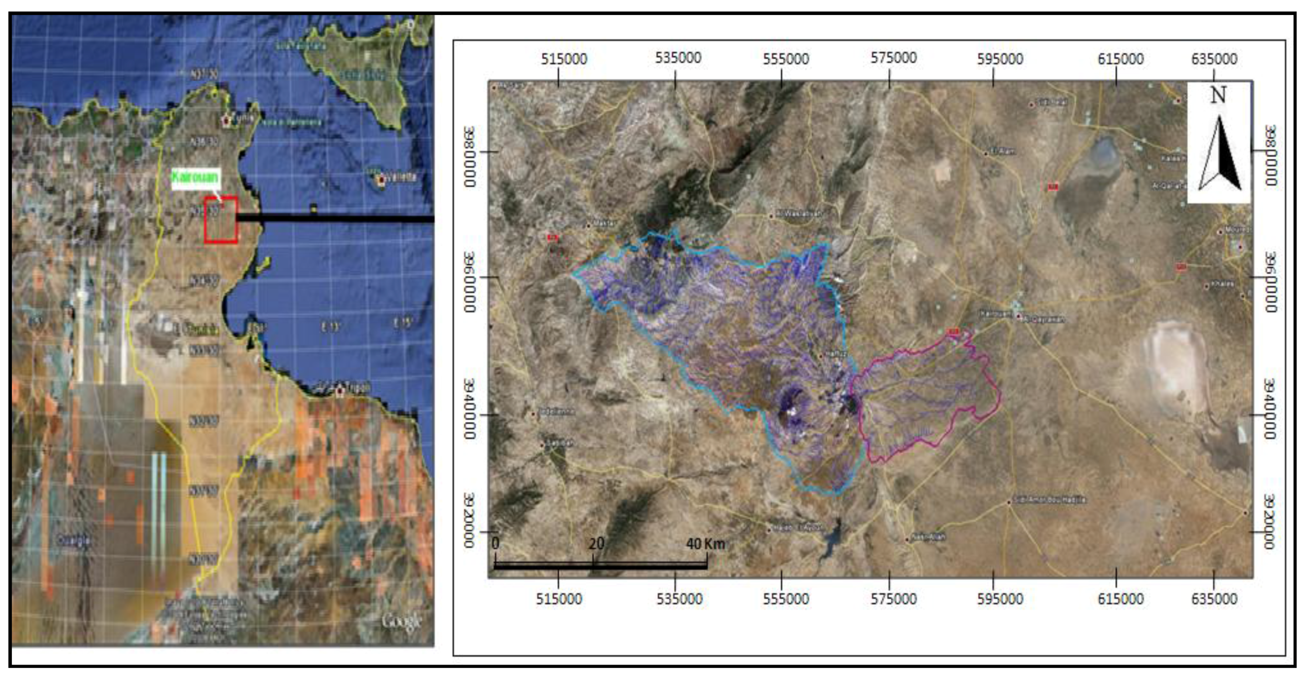
2.1. Study Area

The studied area is located on the Kairouan plain in Central Tunisia (9°23′–10°17′E, 35°1′–35°55′N) as shown in Figure 1. The climate in this region is semi-arid, with an average annual rainfall of approximately 300 mm per year, characterized by a rainy season lasting from October to May, with the two rainiest months being October and March. As is generally the case in semi-arid areas, the rainfall patterns in this area are highly variable in time and space: the rainfall extremes recorded in the Kairouan plain are: 108 mm in 1950/51, and 703 mm in 1969/70. Figure 2 shows the variability of annual precipitation over the last thirteen years. The mean temperature in Kairouan City is 19.2 °C (minimum of 10.7 °C in January and maximum of 28.6 °C in August). The winter is cool in the north-west of the site and moderate elsewhere. The relative humidity varies between 55% and 70% in winter, and between 40% and 55% in summer. The mean annual potential evapotranspiration is close to 1,600 mm.
In the past, most of the surface flow feeding the Kairouan plain came from the three main catchments (Zeroud, Merguellil and Nebhana), which are presently cut-off by large dams (Figure 1). The aquifer of the Kairouan plain is the largest catchment basin in central Tunisia, and is fed by surface water infiltration (Zeroud and Merguellil) during floods in the natural regime, or, since the construction of the Sidi Saad and El Haouareb dams, by water runoff from dam releases [46,47]. Surface and groundwater discharges are drained into Sebkha Kelbia, a large salt lake.
Figure 1. Location of the studied site and land-cover map during the 2009–2010 vegetation season.
Remotesensing 03 02568 g001aRemotesensing 03 02568 g001b
The landscape is mainly flat. The crops are various and their rotation is typical of semi-arid regions. Figure 1 shows a typical land-cover map, produced from SPOT satellite high resolution data. Three land cover classes are dominant over the region of interest, and are analyzed in the present study: (i) Pasture cover: a mixed shrub-land cover, typical of semi-arid regions in North Africa, characterized by a single greenness peak in spring. (ii) Annual agriculture: mainly winter wheat and barley. These crops are sown around mid-November, and are harvested in late May or early June. This form of agriculture is characterised by single-peak greenness in mid March. (iii) Olive trees: these correspond to the most common class of land use in the studied area. There is a very high mean inter-tree spacing of approximately 20m, and the resulting land coverage is quite low (5%).

2.2. NDVI Data

The ten-day synthesis (S10) is a full resolution product (1 km resolution), providing 10-day NDVI data [48]. The quality of the S10-products is directly related to the quality of the P (physical) products. P products are given for top-of-atmosphere (TOA) conditions, for which atmospheric corrections have been applied. These are based on the use of the SMAC algorithm [49], which corrects for molecular and aerosol scattering, water vapor, ozone and other gas absorption effects. Data inputs for the atmospheric correction of SPOT VGT are the aerosol optical depth (AOD), atmospheric water vapor, ozone and a Digital Elevation Model for atmospheric pressure estimation [50]. Water vapor (6-hourly measurements) is obtained from Meteo-France with a 1.5° × 1.5° grid cell resolution. The AOD is derived from the B0 band, in combination with the NDVI [50], although prior to 2001 it was a static data set which varied only as a function of latitude. The P products are corrected for system errors (mis-registration of the different channels, calibration of the linear array detectors for each spectral band), and re-sampled to a Plate–Carrée geographic projection. High absolute location and multi-temporal registration accuracies are obtained, with an estimated absolute location accuracy of 330 m RMS [51]. The cloud flag information is based on thresholding of the TOA reflectance in each of the four bands, which are compared to reference reflectance maps for each band [52,53]. The SPOT-4 and SPOT-5 satellites have an equatorial crossing time of 10:30, and their sensor design provides an improvement over that provided by the AVHRR scanning array, in terms of spatial resolution distortion at off-nadir angles, since it acquires distortion free images at off-nadir angles up to about 50° [53]. Furthermore, the SPOT VGT instruments have other advantages with respect to the AVHRR sensors, including improved navigation and radiometric sensitivity [54]. The ten-day synthesis products (S10) are available at: http://free.vgt.vito.be/.

2.3. Precipitation Data

The precipitation estimations for the studied site are based on a network of 30 rain gauges distributed over the entire site. A standard kriging approach is used to derive daily precipitation maps. One of the most commonly used techniques for interpolation between stations is the “inverse distance weighted” (IDW) method, which is based on the assumption that the interpolating surface is influenced mainly by nearby stations, and less by the more distant stations. As the landscape is mainly flat, there is no mountainous terrain influencing the spatial distribution of rainfall. The interpolated surface is determined from a weighted average of the scatter points, and the weight assigned to each scatter point diminishes inversely with its distance from a given interpolation point [55].
This can be written as:
P ( x , y ) = i = 1 n W i P i
where Pi is the precipitation at the ith station, Wi the weighting factor of the ith station, n the total number of stations used to compute the rainfall at the interpolated point and x,y are the coordinates of the specific point. The precipitation time series is thus available at the same 1 km scale as the NDVI data set.
Figure 2. (a) Rainfall variations during the 13-year study period; (b) Annual cycle of monthly precipitation.
Remotesensing 03 02568 g002aRemotesensing 03 02568 g002b
Figure 2(a) illustrates the high temporal variability of the estimated annual precipitation of the studied site (with a mean value of 252 mm and a standard deviation of 86 mm). In this figure we have used the hydrological years, which span from September to August. 2000–2001 was the driest hydrological year, with a total of 100 mm of precipitation. The wettest hydrological year was 2003–2004, with 380 mm of annual precipitation. The mean monthly precipitations are shown in Figure 2(b). The rainy season is considered to be the period between September and May.

3. Methodology

3.1. Analysis of Persistent Behavior: Method

To quantitatively characterize NDVI dynamics, a technique is needed to extract robust features hidden in the complex NDVI fluctuations. Fractal geometry can be used to describe this complex variability of vegetation dynamics [29,56,57]. Fractals have the property of self-similarity, i.e., the behaviour of a system is temporally scale-independent, such that measurements made at different scales remain comparable. In the present study, our fractal characterization is based on the power spectrum dependence of fractional Brownian motion; we determine the power spectrum of the NDVI time series by computing its Fourier transform. The scaling behaviour of the data is revealed by a power-law dependence of the spectrum as a function of frequency [58,59]:
S ( f ) 1 / f β
The fractal dimension is derived from the slope β of a least-squares regression linear fit to the data points in the log-log plot of the power spectrum, leading to Df = 7/2 − β/2.
The slope β allows the time-correlation structures, corresponding to the temporal variability of the signals, to be analysed [35]. We consider three cases: β = 0, β > 0, and β < 0.
When (β = 0) the signal is purely random, with uncorrelated samples. We refer to such a process as being ‘memoryless’: there is no relationship between the fluctuations occurring at different time-scales.
When (β > 0) the temporal variability is persistent. This means that a positive (negative) signal variability will probably produce a positive (negative) variation in vegetation dynamics. This corresponds to the case of positive feedback in a vegetation system.
When (β < 0) the temporal variability is non-persistent. This means that a positive (negative) signal variability will probably lead to negative (positive) variations in the vegetation’s behavior. This is equivalent to a negative feedback mechanism.

3.2. Development of a Vegetation Anomaly Index (VAI)

Periods of drought have a strong influence on vegetation dynamics, with persistence effects over long periods. We clearly observe differences between dry and wet years, for the three principal types of vegetation present on our studied site.
In this section, we propose to use a simple index, which can provide a quantitative illustration of vegetation stress and the influence of drought on the vegetation cover. This index is based on statistics derived from the NDVI time series, and is referred to as the “Vegetation Anomaly Index” (VAI), written as:
V A I i = N D V I i ( N D V I i ) m e a n σ i
Where NDVIi is the NDVI estimate for a given month i, (NDVIi)mean is the mean value of the NDVI during month i, derived from the previously described 13 years of NDVI time series, and σi corresponds to the standard deviation of the NDVI values estimated for month i, over the same 13 year period.
When the VAI is greater than zero, a high NDVI value, corresponding to the absence of vegetation stress or drought, is indicated.
When the VAI is negative, a low NDVI value, which is probably the result of drought or a period with a lack of precipitation, is indicated. We have computed this index for the three types of vegetation cover described in Section 2.1.

4. Results and Discussions

4.1. NDVI Temporal Series

Figure 3(a–c) shows the NDVI time series and monthly precipitations recorded over the last 13 years (September 1998–June 2010), for three types of vegetation: pastures, annual agricultural areas, and olive trees. For each case, the NDVI and precipitation data correspond to an average over a selected area, with one type of homogenous vegetation cover. Figure 3(d–f) are photographs, illustrating the corresponding types of vegetation cover. In all cases, qualitative differences can be observed in the NDVI series, between the wet and dry seasons. Indeed, the NDVI maximum, for example, reaches only 0.25 over the pastures in 2001, a very dry year, as compared to the value of 0.55 in 2007, the wettest of the last 13 years.

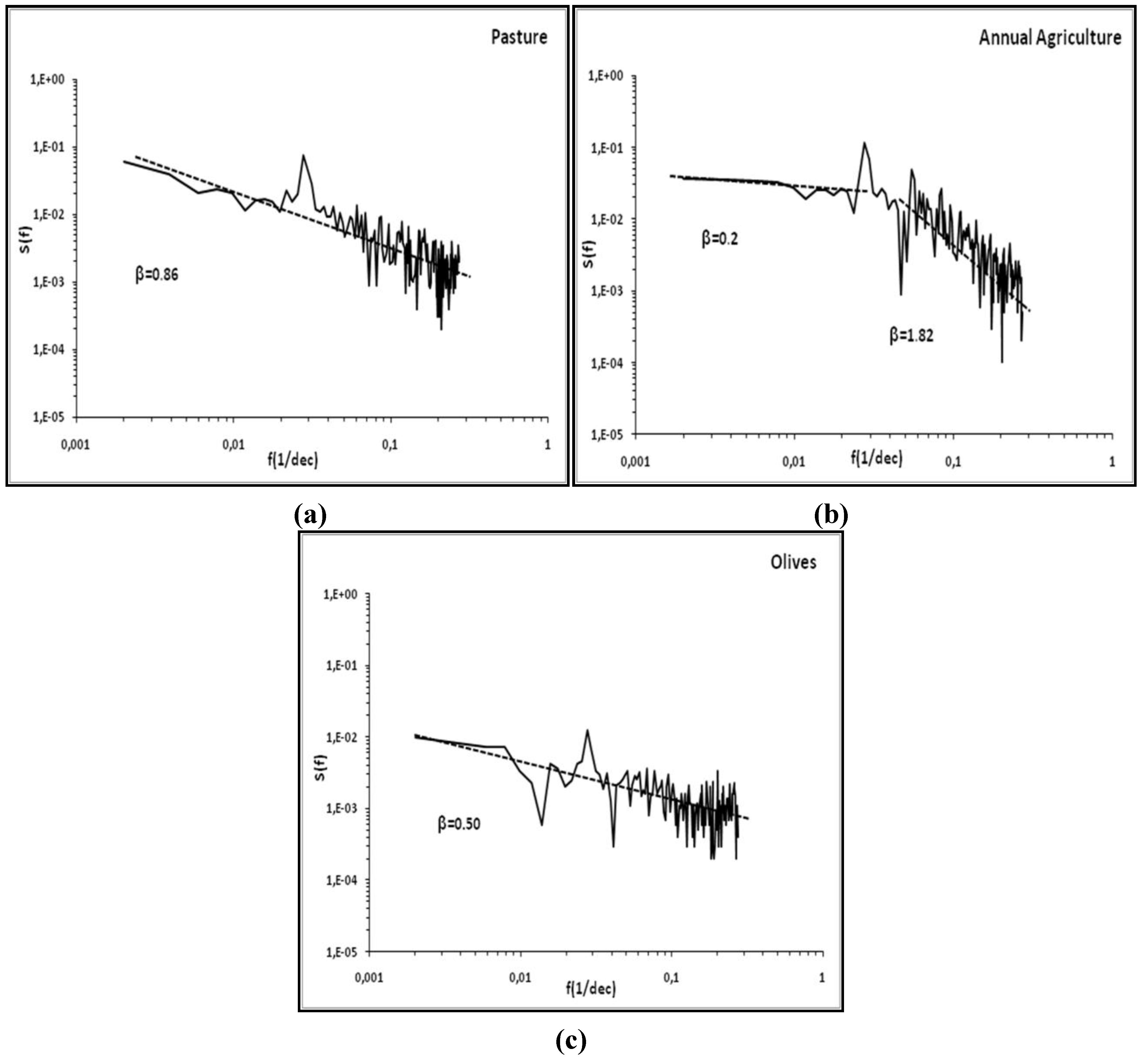
4.2. Application of Persistence Analysis to Various Types of Vegetation

The power spectral density of each NDVI series was computed in order to analyze the persistence behavior of the three corresponding types of vegetation cover.
Figure 3. Temporal variations of the spatially averaged NDVI for three types of vegetation cover, from September 1998 to June 2010: (a) pasture, (b) annual agriculture and (c) olive groves. The scale of the abscissa is in units of 1 “decade” (= 10 days).
Remotesensing 03 02568 g003

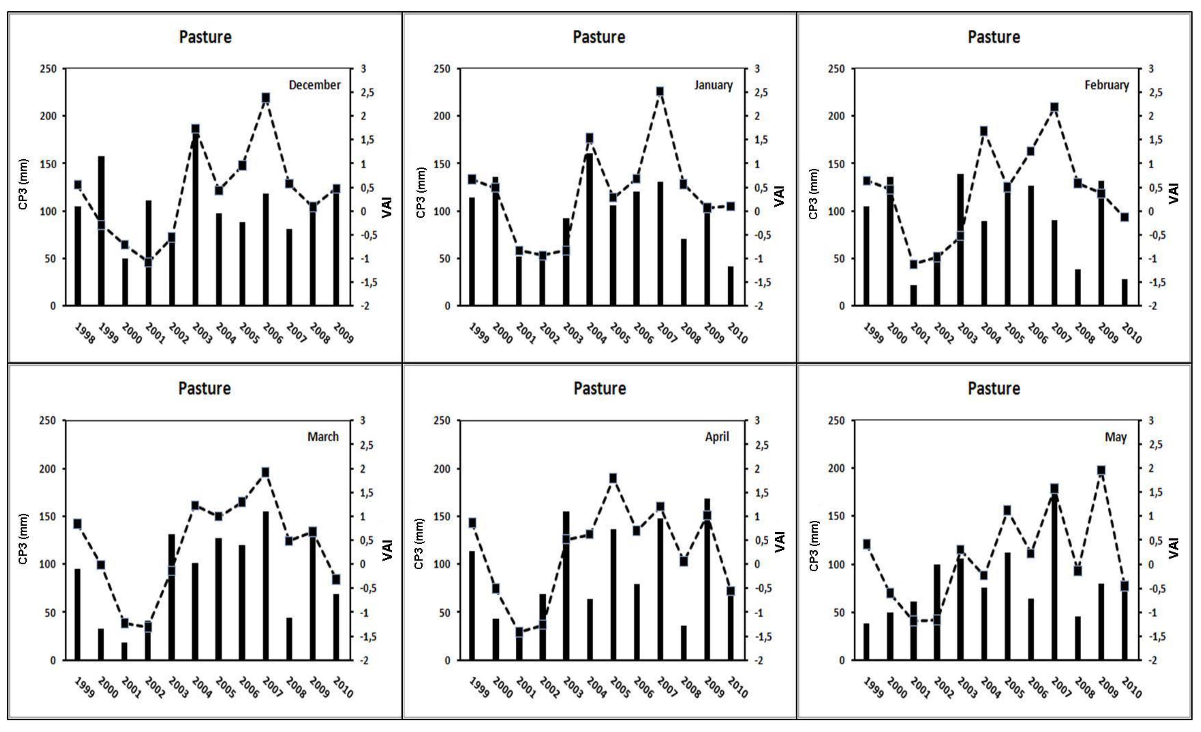
4.2.1. Pastoral Cover

Figure 4(a) shows the computed power spectral density. For this type of vegetation, the slope β is found to be equal to 0.86. A high power peak can also be observed, corresponding to the annual periodicity of the vegetation cycle. The influence of the annual periodicity was not eliminated directly from the temporal signal before computing the power density, as proposed by [40]. In fact, it is possible to extract the high frequency signal only, provided there are no extreme events, which is not the case on our site. The peak corresponding to the annual frequency is not taken into account in the computation of the slope. The latter indicates the presence of persistent dynamics, with positive feedback mechanisms. The linear relationship for the log-log plot is valid for scales ranging between approximately two decades and 2 years. This result indicates, in particular, a drought persistence effect with this type of vegetation, which can last for more than one year. In the field, this outcome can be explained by the fact that a high percentage of the pasture has no annual vegetation, but is covered instead by short vegetation, which grows over a period of several years. Following a major drought event, and the disappearance of part of the vegetation cover, the latter may require more than one year to retrieve the degree of coverage it represented prior to the drought.

4.2.2. Annual Agricultural Cover

The results shown in Figure 4(b) indicate two different types of behavior: the first is highlighted by the clearly positive slope in the range between two decades and one year, and the second trend is shown by the slope close to zero, at frequencies corresponding to a period of more than one year. The peak which occurs at the break between these two trends indicates the annual periodicity of the vegetation’s NDVI index. The first trend (positive slope = 1.82) indicates persistent behavior, corresponding to the scale of one agricultural season. In practice, the effects of any period of drought can be felt throughout the full season. Following this season, there is no memory of what happened one year previously. In fact, at the beginning of the autumn, the quantity of water in the soil is always very close to zero, independently of whether the preceding season was wet or dry. For this reason, the second trend (frequencies less than 1/year) corresponds to a memoryless process.

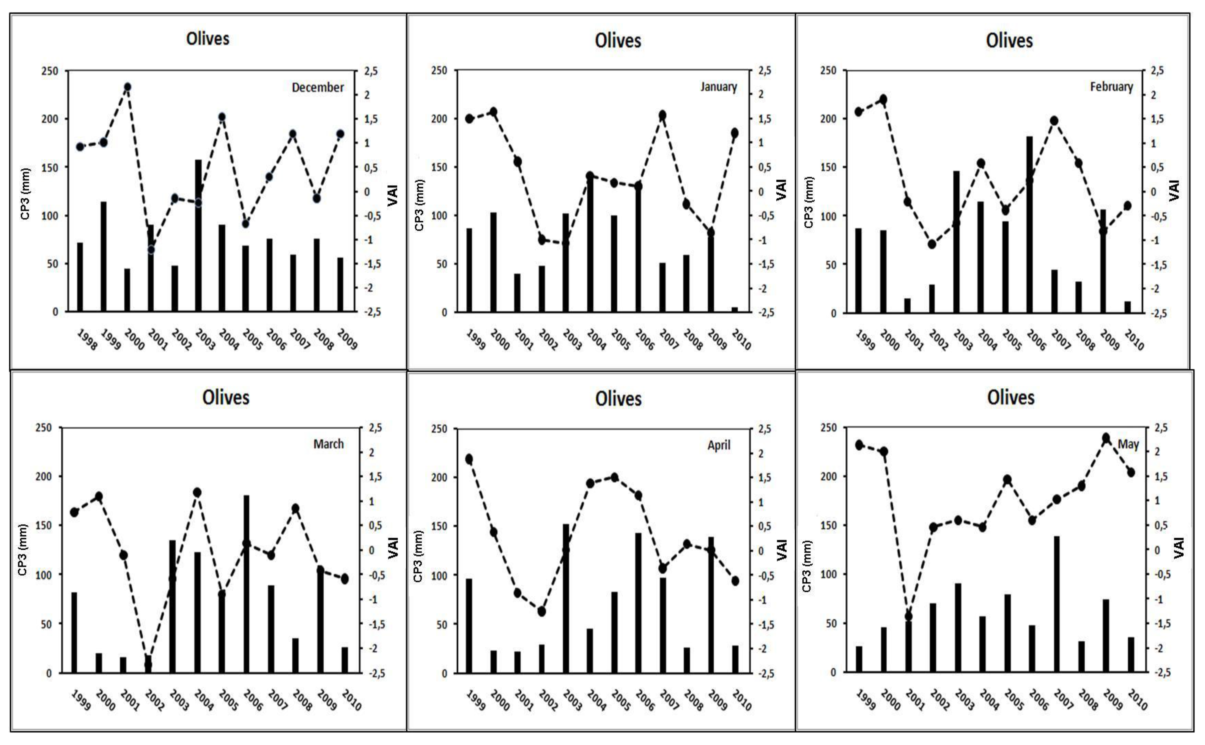
4.2.3. Non Irrigated Olive Grove

For the case of a non irrigated olive grove, Figure 4(c) is characterized by a low slope of 0.50, and therefore a small degree of persistence, when compared to that of the pastures, present at all scales between two decades and two years. The low persistence effect indicates the olive trees’ resistance to drought. Indeed, in these semi-arid areas, olive trees are highly resistant to frequent periods of drought, in particular because of the large distance between trees (approximately 20 m), which allows their roots to search for water stock over a large area.
Figure 4. Power spectral density plots for: (a) pasture; (b) annual agriculture; (c) olive trees.
Remotesensing 03 02568 g004

4.3. Evaluation of the VAI

In this section, following the analysis of drought persistence for the three types of vegetation cover on the studied site, we discuss the VAI variations for each month during the rainy season. We firstly validate the correlation between this index and both precipitation, and the other proposed indices.
For each month i, we compute the Cumulative Precipitation CPn,i written as:
C P n , i = P i n + P i n + 1 + .... + P i 1 + j = 1 30 ( P d j × ( 30 j ) 30 )
where Pi−n is the total precipitation in month i−n,…, Pi−1 is the total precipitation in month i−1, and Pdj is the precipitation on day j, during the month i.
For a given month i, we assigned a weight to the precipitation of the previous month, because the vegetation NDVI index for the month i is influenced mainly by the precipitation which fell during the preceding months. In practice, the precipitation measured during the last days of any given month can only have a very limited effect on the vegetation index estimated during that same month. For example, for n = 3, this corresponds to the total rainfall of 4 months which is called CP3.

4.3.1. Correlation of the VAI with Precipitation

In order to validate the proposed index, we studied the correlation of the VAI with the recorded levels of precipitation, given by the cumulative precipitation CPn,i (for n less than 6). The strongest correlation is found for n equal to 3. Table 1 illustrates the correlation coefficients, between the VAI and the CP3 cumulative precipitation, for the three types of vegetation cover. In general, a high degree of correlation is observed between VAI and precipitation, for the pastoral and annual agricultural types of cover. A positive VAI generally corresponds to a high level of precipitation, whereas a decrease in precipitation generally leads to a decrease in the VAI. In the case of the olive grove cover, the correlation coefficient is lower, which, as previously discussed, can be attributed to the limited influence of drought on this highly resistant type of vegetation, and also to its limited vegetation fraction (about 5%). Table 1 indicates that precipitation does not have an immediate impact on vegetation, but rather a cumulative effect. In most cases, the precipitation recorded in any given month does not strongly affect the vegetation in that same month, but leads to a notable response over a longer period of time. Previous studies have determined the peak NDVI response to precipitation in many different zones. Yang et al. [60] found that the NDVI’s response to precipitation lagged by 5–7 weeks, for all types of vegetation in Nebraska. A recent study by Wang et al. [61] indicates a lag of 4–8 weeks. For periods between 6 and 12 months, the correlations do not improve [60]; this is due to the fact that the longer scale of precipitation tends to diminish the variance of the latter. The correlation analysis illustrates the robustness of the proposed index. The highest correlations occurred during the middle of the growing season (R2 around 0.64), whereas lower correlations are noted at the beginning and end of the growing season. For example, in March and April high positive correlations are noted between the vegetation index and precipitation. March and April are the peak greenness months for annual agriculture. This implies that the vegetation expresses its strongest response to water availability during the peak greenness period. In June, July and August, there is no significant correlation, at the time when most types of vegetation in this region are approaching full senescence.

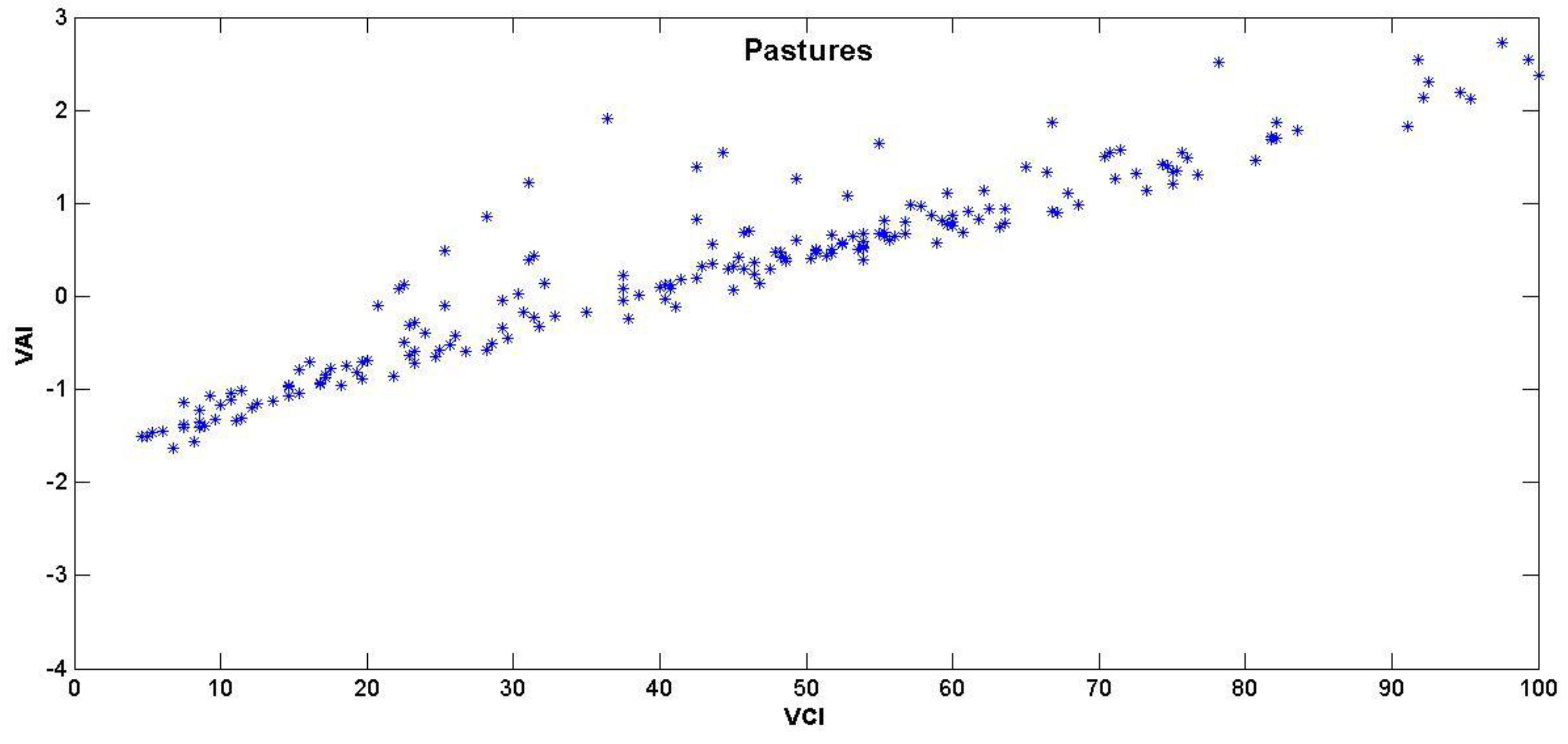
4.3.2. Comparison between the VAI and VCI Indices

Figure 5 provides a graphical comparison of the VAI and VCI indices, as defined in the introduction. These two indices are computed on a monthly basis, using all observations recorded in the database corresponding to the rainy season between December and May. For the three types of vegetation, these two indices are seen to correlated, either for the full range of values, or for a limited range of values. For the pastures and olive trees, an approximately linear relationship can be observed. In the case of annual agricultural cover, two different tendencies can be seen, with an onset of saturation for positive values of the VAI occurring when the VCI reaches a value of approximately 40. This is due to the fact that only minimum and maximum NDVI values are taken into account in the computation of the VCI, and also to a strong difference between the wet and dry season NDVIs determined for annual agriculture, as compared to those computed for the other two types of cover. These two factors lead firstly to a high discrepancy between the statistically mean value of the NDVI, and the mean level computed for the VCI index, and secondly to a high standard deviation used for the VAI computation (Equation (3)), which tends to prevent the VAI from increasing beyond a value of about 2. For the same reasons, it can be seen that a zero value for the VAI does not correspond to a value of exactly 50 for the VCI index. The difference between the statistical mean values, and the mean value computed from the minimum and maximum NDVI levels only, could vary from one region to another and from one type of vegetation cover to another. On the basis of the observed differences between these two indices, the VAI is found to have a better performance in terms of the measurement of drought intensity.
Table 1. VAI to CP3 precipitation correlation coefficients, computed for each month, for annual agriculture, pastures and olive groves.
Annual AgriculturePasturesOlives
MonthCorrelation Coefficient R2
September0.0060.2380.032
October0.1310.6780.218
November0.0350.2450.004
December0.3490.1850.084
January0.4440.4970.020
February0.3260.1190.000
March0.6810.5720.028
April 0.5730.5440.115
May0.3330.2220.013
June 0.0780.0540.011
July0.1050.1260.032
August0.1150.0190.004
Figure 5. Intercomparison of VAI and VCI indexes, estimated from the full set of recordings corresponding to the rainy season months (December–May).
Remotesensing 03 02568 g005aRemotesensing 03 02568 g005b

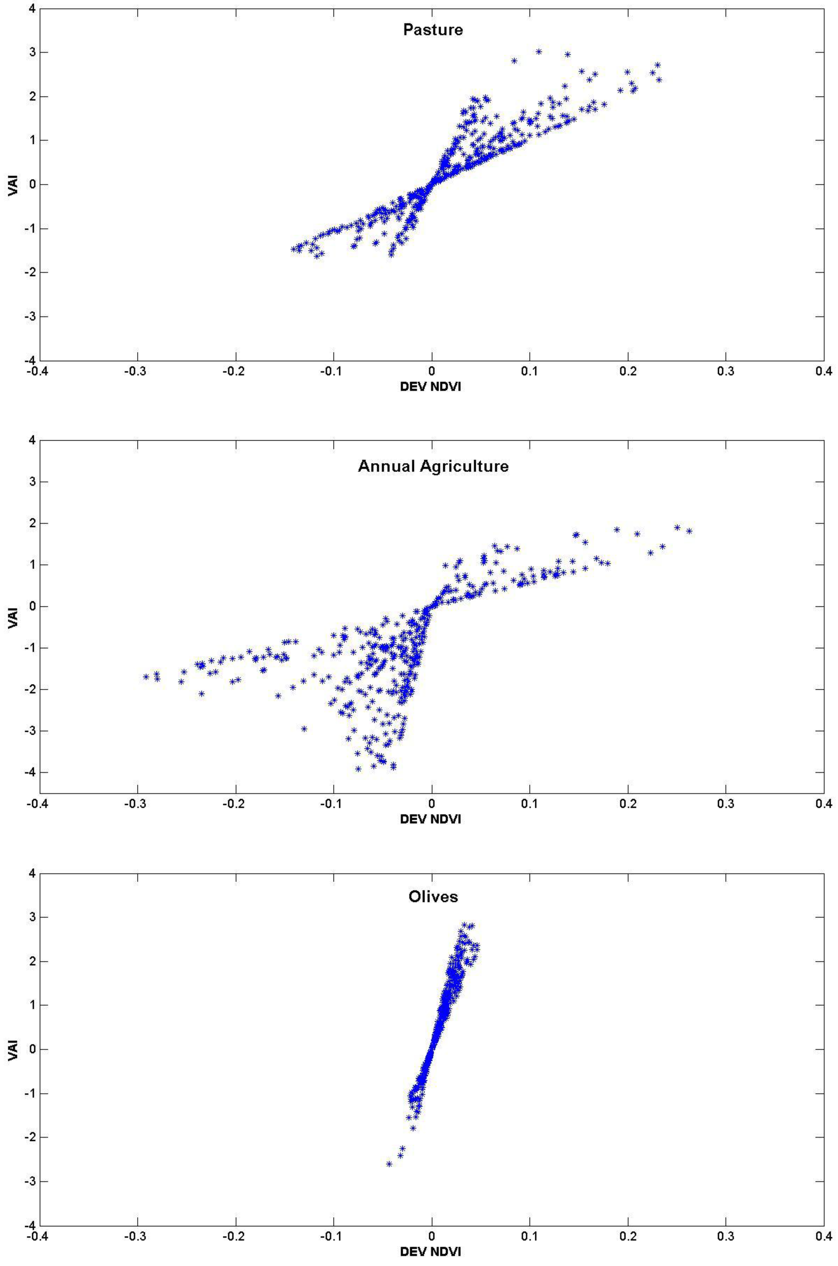
4.3.3. Comparison between the VAI and DEV.NDVI Indices

Figure 6 provides a graphical comparison between the VAI and DEV.NDVI indices, as defined in the introduction. Comparatively small differences are observed between the two indices. The VAI is simply the product of DEV.NDVI and the standard deviation computed for each month, thus explaining that these figures contain index data points whose mean value is equal to zero. A high degree of coherency can be observed between the two indices for each month. Dry seasons lead to negative values for both indices, and rainy seasons lead to positive values for both indices. However, from one month to another, variations in the linear relationship between the two indices can be observed, as a consequence of variations in the value of standard deviation computed from one month to another. This outcome highlights limitations in the DEV.NDVI index for the month-by-month estimation of drought intensity. This is particularly noticeable in the case of olive tree land cover, for which there are only small variations in NDVI. In fact, division by the monthly standard deviation, used in the determination of the VAI (Equation (3)), allows a normalized value to be computed, which is independent of the selected time period or type of vegetation. For this reason, the VAI could provide a more detailed description of the vegetation cover dynamics, with no need for other complementary or auxiliary forms of data.
Figure 6. Intercomparison between VAI and DEV.NDVI indexes, estimated from the full set of database recordings corresponding to the rainy season months (December–May).
Remotesensing 03 02568 g006

4.4. VAI Applications

4.4.1. Application of the VAI to Pasture Cover

Figure 7 shows the VAI variations determined for the case of pasture cover. A good degree of coherence can be seen between the VAI and the cumulative precipitation CP3. In the month of March, the minimum values, close to −1.3, are observed for the driest years, 2001 and 2002, which also correspond to the period with the lowest level of precipitation, from the full time series. These results also correspond with those observed for annual agriculture, as discussed in the previous section.
Figure 7. Variations in the VAI for each month between December and May, for the case of a “pastoral” vegetation cover.
Remotesensing 03 02568 g007

4.4.2. Application of VAI over Annual Agriculture Cover

Figure 8 shows, for each month from December to May, as a function of the 13 processed years in our database, the VAI together with the CP3 “cumulative four month precipitation”. Depending on the month of the year, the VAI can be seen to range between approximately −3 and 2. As an example, during the month of December the VAI ranges between a minimum of −2.75 in 2000, the driest year, and a maximum of 0.5 in 2008. In general, limited periods of drought, or a lack of precipitation lasting for a period of several weeks, were observed every year. This leads to a local decrease in the VAI. Qualitatively, a strong correlation can be observed between the VAI and the cumulative precipitation, CP3: a strong decrease in the cumulative precipitation is generally associated with a negative VAI. This can be seen for example in 2001 and 2002, for almost all months (values between −1.3 and −2). On the other hand, a strong increase in CP3 leads to a positive VAI, as can be seen in several different cases, for example in the month of March 2003 or 2004.
Figure 8. Variations in the VAI, for each month between December and May, for the case of an “annual agriculture” vegetation cover.
Remotesensing 03 02568 g008

4.4.3. Application of the VAI to Olive Tree Land Cover

Figure 9 shows the VAI variations determined for the Kairouan plain olive groves. As a result of the small variations in NDVI for the case of olive tree coverage, due to the highly dispersed nature of this vegetation and its high resistance to periods of drought, the VAI is less sensitive to drought and long periods of rain. This is the reason for which a weaker degree of correlation can be seen with precipitation (CP3), as compared to the other types of vegetation cover.

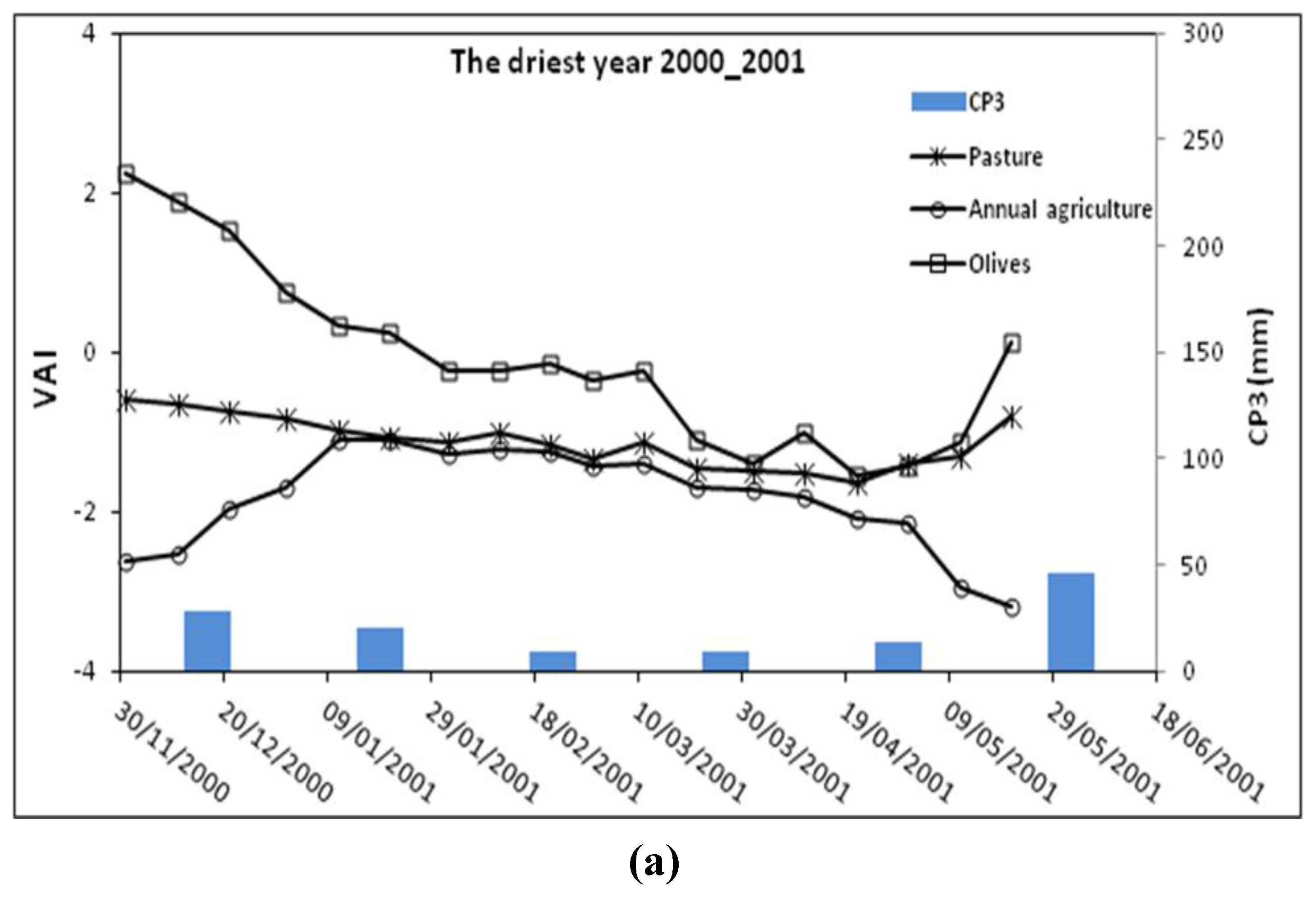
4.4.4. Analysis of VAI Indices for the Driest and Wettest Years

Figure 10 shows the VAI variations and corresponding CP3 estimations for two different periods; 2000–2001, the driest period with a total precipitation equal to 100 mm, and 2003–2004, the wettest period with a total precipitation equal to 380mm. For the first of these, we observe a consistently negative index, for all months, in the case of the pastoral and annual agriculture vegetation covers, which indicates high vegetation stress and drought for the full duration of the season. In the case of olive tree cover, as mentioned in the previous section, the correlation with drought periods is less significant, and the VAI is not consistently negative. During the 2003–2004 season, the index is positive for the first three months starting in December, because of the occurrence of high levels of precipitation during this period. During the other years, both positive and negative VAI can be observed, which appear to be strongly correlated with the presence (or absence) of precipitation.
Figure 9. Variations in the VAI for each month between December and May, for Olive groves.
Remotesensing 03 02568 g009
Figure 10. Variations in the monthly VAI for each type of vegetation cover, with data points at 10-day (decade) intervals from December to the end of May, for two different periods: (a) the drought year 2000–2001, (b) the wet year 2003–2004.
Remotesensing 03 02568 g010aRemotesensing 03 02568 g010b

5. Conclusions

This paper proposes to analyze the behavior of vegetation as a consequence of drought, using SPOT-VEGETATION NDVI data. Analysis of the power spectral density of the NDVI corresponding to three forms of land cover (pasture, annual agriculture, olive trees) reveals persistent temporal fluctuations, for time scales ranging between three decades and approximately two years, with the greatest persistence being observed for annual agriculture.
An index based on the statistics of NDVI time series, which we refer to as the Vegetation Anomaly Index (VAI), is proposed for the monitoring and analysis of drought intensity. A positive VAI indicates satisfactory vegetation dynamics, whereas a negative VAI indicates the presence of vegetation stress. The performance of the VAI is firstly compared with the other two well-known remote sensing indices (VCI and DEV. NDVI) found in scientific literature. This comparison confirms the VAI’s ability to more accurately detect drought and analyze its intensity. The VAI is also compared with precipitation, with which it is found to be well correlated: the correlation is strongest for 4-month cumulative precipitation (CP3). This is a consequence of the time lag between the vegetation’s response to precipitation, and the fact that water deficits have a cumulative impact on vegetation, especially in arid regions. Despite its strong potential, the VAI may be affected by some limitations, as a consequence of its potential sensitivity to effects other than drought, such as evolutions in land use from one year to another, the strong influence of irrigation in agricultural areas, and also land use heterogeneities over the studied area.
In future studies, we plan to analyze potential applications of the VAI index at the spatial scale of a single pixel. An analysis of the various limitations of this index, in particular the influence of surface heterogeneities, will also be investigated.

Acknowledgments

This study was funded by three programs: the French national MISTRALS program, the European WASSERMED project, and the French Institut de Recherche pour le Développement (Institute for Research and Development). We would like to thank VITO for kindly providing us with its SPOT-VEGETATION NDVI products, and the ISIS program for providing us with SPOT images. We wish to thank the Tunisian Ministry of Agriculture for providing us with the precipitation data used in this study. We also thank all of the technical teams of the IRD, the INAT, CTV-Chebika and INGC for their strong collaboration and support in implementing the ground-truth measurements.

References

  1. Lambin, E.F.; Ehrlich, D. The surface temperature-vegetation index space for land cover and land-cover change analysis. Int. J. Remote Sens. 1996, 17, 463–487. [Google Scholar] [CrossRef]
  2. Duchemin, B.; Hadria, R.; Erraki, S.; Boulet, G.; Maisongrande, P.; Chehbouni, A.; Escadafal, R.; Ezzahar, J.; Hoedjes, C.B.; Kharrou, M.H.; Khabba, S.; Mougenot, B.; Olioso, A.; Rodriguez, J.C.; Simonneaux, V. Monitoring wheat phenology and irrigation in Central Morocco: On the use of relationships between evapotranspiration, crops coefficients, leaf area index and remotely-sensed vegetation indices. Agr. Water Manage. 2005, 79, 1–27. [Google Scholar] [CrossRef]
  3. Downing, T.E.; Bakker, K. Drought discourse and vulnerability. In Drought: A Global Assessment; Wilhite, D.A., Ed.; Natural Hazards and Disasters Series; Routledge: London, UK, 2000. [Google Scholar]
  4. Palmer, W.C. Meteorologic Drought; US Department of Commerce, Weather Bureau, Research Paper; 1965; p. 58. [Google Scholar]
  5. Van Rooy, M.P. A rainfall anomaly index independent of time and space. Notos 1965, 14, 43. [Google Scholar]
  6. Gibbs, W.J.; Maher, J.V. Rainfall Deciles as Drought Indicators; Bureau of Meteorology Bull. 48; Commonwealth of Australia: Melbourne, Australia, 1967. [Google Scholar]
  7. Palmer, W.C. Keeping track of crop moisture conditions, nationwide: The new crop moisture index. Weatherwise 1968, 21, 156–161. [Google Scholar] [CrossRef]
  8. Bhalme, H.N.; Mooley, D.A. Large-scale droughts/floods and monsoon circulation. Mon. Weather Rev. 1980, 108, 1197–1211. [Google Scholar] [CrossRef]
  9. Shafer, B.A.; Dezman, L.E. Development of a Surface Water Supply Index (SWSI) to Assess the Severity of Drought Conditions in Snowpack Runoff Areas. In Proceedings of Western Snow Conference, Reno, NV, USA, 19–23 April 1982; pp. 164–175.
  10. Gommes, R.; Petrassi, F. Rainfall Variability and Drought in Sub-Saharan Africa since 1960; Agro-meteorology Series 9; Food and Agriculture Organization: Rome, Italy, 1994. [Google Scholar]
  11. McKee, T.B.; Doesken, N.J.; Kleist, J. The Relationship of Drought Frequency and Duration to Time Scales. In Proceedings of 8th Conference on Applied Climatology, Anaheim, CA, USA, 17–22 January 1993; pp. 179–184.
  12. McKee, T.B.; Doesken, N.J.; Kleist, J. Drought Monitoring with Multiple Time Scales. In Proceedings of 9th Conference on Applied Climatology, Dallas, TX, USA, 15–20 January 1995.
  13. Weghorst, K.M. The Reclamation Drought Index: Guidelines and Practical Applications; Bureau of Reclamation: Denver, CO, USA, 1996; p. 6. [Google Scholar]
  14. Palmer, W.C. Meteorological Drought; Research Paper No. 45; US Weather Bureau: Washington, DC, USA, 1965; p. 58. [Google Scholar]
  15. Vicente-Serrano, S.M.; Beguería, S.; López-Moreno, J.I. A Multi-scalar drought index sensitive to global warming: The Standardized Precipitation Evapotranspiration Index—SPEI. J. Climate. 2010, 23, 1696–1718. [Google Scholar] [CrossRef]
  16. Meyer, S.J.; Hubbard, K.G. Extending the Crop-specific Drought Index to Soybean. In Proceedings of 9th Conference on Applied Climatology, Dallas, TX, USA, 15–20 January 1995; pp. 258–259.
  17. Rouse, J.W.; Haas, R.H.; Schell, J.A.; Deering, D.W. Monitoring the vernal advancement and retrogradation (green wave effect) of natural vegetation. In Progress Report RSC 1978-1; Remote Sensing Center, Texas A&M University: College Station, TX, USA, 1974. [Google Scholar]
  18. Sellers, P.J. Canopy reflectance, photosynthesis and transpiration. Int. J. Remote Sens. 1985, 6, 1335–1372. [Google Scholar] [CrossRef]
  19. Deblonde, G.; Cihlar, J. A multiyear analysis of the relationship between surface environmental variables and NDVI over the Canadian landmass. Remote Sensing Rev. 1993, 7, 151–177. [Google Scholar] [CrossRef]
  20. Myneni, R.B.; Los, S.O.; Asrar, G. Potential gross primary productivity of terrestrial vegetation from 1982 to 1990. Geophyis. Res. Lett. 1995, 22, 2617–2620. [Google Scholar] [CrossRef]
  21. Prince, S.D.; Tucker, C.J. Satellite remote sensing of rangelands in Botswana: II. NOAA AVHRR and herbaceous vegetation. Int. J. Remote Sens. 1986, 7, 1555–1570. [Google Scholar] [CrossRef]
  22. Salah Er-Raki, S.; Chehbouni, A.; Duchemin, B. Combining satellite remote sensing data with the FAO-56 dual approach for water use mapping in irrigated wheat fields of a semi-arid region. Remote Sens. 2010, 2, 375–387. [Google Scholar] [CrossRef]
  23. Laurila, H.; Karjalainen, M.; Kleemola, J.; Hyyppä, J. Cereal yield modeling in Finland using optical and radar remote sensing. Remote Sens. 2010, 2, 2185–2239. [Google Scholar] [CrossRef]
  24. Propastin, P.; Kappas, M. Modeling net ecosystem exchange for grassland in Central Kazakhstan by combining remote sensing and field data. Remote Sens. 2009, 1, 159–183. [Google Scholar] [CrossRef]
  25. Fraser, R.S.; Kaufman, Y.J. The relative importance of scattering and absorption in remote sensing. IEEE Trans. Geosci. Remote Sens. 1985, 23, 625–633. [Google Scholar] [CrossRef]
  26. Holben, B.N.; Kaufaman, Y.J.; Kendall, J.D. NOAA-11 AVHRR visible and near-IR inflight calibration. Int. J. Remote Sens. 1990, 11, 1511–1519. [Google Scholar] [CrossRef]
  27. Cuomo, V.; Lanfredi, M.; Lasaponara, R.; Macchiato, M.; Simoniello, T. Detection of interannual variation of vegetation in middle and southern Italy during 1985–99 with 1 km NOAA AVHRR NDVI data. J. Geophys. Res. 2001, 106, 17863–17876. [Google Scholar] [CrossRef]
  28. Huemmrich, K.E.; Black, T.A.; Jarvis, P.G.; McCaughey, J.H.; Hall, E.G. Remote sensing of carbon/water/energy parameters—High temporal resolution NDVI phenology from micrometeorological radiation sensors. J. Geophys. Res. 1999, 104, 27935–27944. [Google Scholar] [CrossRef]
  29. Lanfredi, M.; Simoniello, T.; Macchiato, M. Temporal persistence in vegetation cover changes observed from satellite: Development of an estimation procedure in the test site of the Mediterranean Italy. Remote Sens. Environ. 2004, 93, 565–576. [Google Scholar] [CrossRef]
  30. Myneni, R.B.; Los, S.O.; Tucker, C.J. Satellite-based identification of linked vegetation index and sea surface temperature anomaly areas from 1982 to 1990 for Africa, Australia and South America. Geophys. Res. Lett. 1996, 23, 729–732. [Google Scholar] [CrossRef]
  31. Tucker, C. Red and photographic infrared linear combinations for monitoring vegetation. Remote Sens. Environ. 1979, 8, 127–150. [Google Scholar] [CrossRef]
  32. Kogan, F.N. Application of vegetation index and brightness temperature for drought detection. Adv. Space Res. 1995, 15, 91–100. [Google Scholar] [CrossRef]
  33. Seiler, R.A.; Kogan, F.; Wei, G. Monitoring weather impact and crop yield from NOAA AVHRR data in Argentina. Adv. Space Res. 2000, 26, 1177–1185. [Google Scholar] [CrossRef]
  34. Anyamba, A.; Tucker, C.J.; Eastman, J.R. NDVI anomaly patterns over Africa during the 1997/98 ENSO warm event. Int. J. Remote Sens. 2001, 22, 1847–1859. [Google Scholar]
  35. Wang, J.; Price, K.P.; Rich, P.M. Spatial patterns of NDVI in response to precipitation and temperature in the central Great Plains. Int. J. Remote Sens. 2001, 22, 3827–3844. [Google Scholar] [CrossRef]
  36. Ji, L.; Peters, A. Assessing vegetation response to drought in the northern Great Plains using vegetation and drought indices. Remote Sens. Environ. 2003, 87, 85–89. [Google Scholar] [CrossRef]
  37. Singh, R.P.; Roy, S.; Kogan, F.N. Vegetation and temperature condition indices from NOAA AVHRR data for drought monitoring over India. Int. J. Remote Sens. 2003, 24, 4393–4402. [Google Scholar] [CrossRef]
  38. Quiring, S.M.; Ganesh, S. Evaluating the utility of the Vegetation Condition Index (VCI) for monitoring meteorological drought in Texas. Agric. Forest Meteorol. 2010, 150, 330–339. [Google Scholar] [CrossRef]
  39. Peters, J.; Waltershea, E.A.; Ji, L.; Vliia, A.; Hayes, M.; Svoboda, M.D.; Nir, R. Drought monitoring with NDVI-based Standardized Vegetation Index. Photogramm. Eng. Remote Sensing. 2002, 68, 71–75. [Google Scholar]
  40. Gouveia, C.; Trigo, R.M.; DaCamara, C.C.; Libonati, R.; Pereira, J.M.C. The North Atlantic oscillation and European vegetation dynamics. Int. J. Clim. 2008, 28, 1835–1847. [Google Scholar] [CrossRef]
  41. Gouveia, C.; Trigo, R.M.; DaCamara, C.C. Drought and vegetation stress monitoring in Portugal using satellite data. Nat. Hazards Earth Syst. Sci. 2009, 9, 185–195. [Google Scholar] [CrossRef]
  42. Trigo, R.M.; Gouveia, C.M.; Barriopedro, D. The intense 2007–2009 drought in the Fertile Crescent: Impacts and associated atmospheric circulation. Agric. Forest Meteorol. 2010, 150, 1245–1257. [Google Scholar] [CrossRef]
  43. Bhuiyan, C.; Kogan, F.N. Monsoon dynamics and vegetative drought patterns in the Luni basin under rain-shadow zone. Int. J. Remote Sens. 2010, 31, 3223–3242. [Google Scholar] [CrossRef]
  44. Telesca, L.; Lasaponara, R. Quantifying intra-annual persistent behaviour in SPOT-VEGETATION NDVI data for Mediterranean ecosystems of southern Italy. Remote Sens. Environ. 2005, 101, 95–103. [Google Scholar] [CrossRef]
  45. Martínez, B.; Gilabert, M.A. Vegetation dynamics from NDVI time series analysis using the wavelet transform. Remote Sens. Environ. 2008, 113, 1823–1842. [Google Scholar] [CrossRef]
  46. Lacombe, G.; Cappelaere, B.; Leduc, C. Hydrological impact of water and soil conservation works in the Merguellil catchment of central Tunisia. J. Hydrol. 2008, 359, 210–224. [Google Scholar] [CrossRef]
  47. Zribi, M.; Chahbi, A.; Shabou, M.; Lili-Chabaane, Z.; Duchemin, B.; Baghdadi, N.; Amri, R.; Chehbouni, A. Soil surface moisture estimation over a semi-arid region using ENVISAT ASAR radar data for soil evaporation evaluation. Hydrol. Earth Syst. Sci. 2011, 15, 345–358. [Google Scholar] [CrossRef] [Green Version]
  48. Holben, B.N. Characteristics of maximum-values composite images from temporal AVHRR data. Int. J. Remote Sens. 1986, 7, 1417–1434. [Google Scholar] [CrossRef]
  49. Rahman, H.; Dedieu, G. SMAC: A simplified method for the atmospheric correction of satellite measurements in the solar spectrum. Int. J. Remote Sens. 1994, 15, 123–143. [Google Scholar] [CrossRef]
  50. Maisongrande, P.; Duchemin, B.; Dedieu, G. VEGETATION/SPOT—An operational mission for the earth monitoring—Presentation of new standard products. Int. J. Remote Sens. 2004, 25, 9–14. [Google Scholar] [CrossRef]
  51. Sylvander, S.; Albert-Grousset, I.; Henry, P. VEGETATION Geometrical Image Quality. In Proceedings of the VEGETATION 2000 Conference, Belgirate, Italy, 3–6 April 2000; pp. 33–34.
  52. Kempeneers, P.; Lissens, G.; Fierens, F.; Van Rensbergen, J. Detection of Clouds and Cloud-Shadows for VEGETATION Images. In Proceedings of VEGETATION 2000 Symposium, Maggiore, Italy, 3–6 April 2000.
  53. SPOT Vegetation User’s Guide. 2008. Available online: http: //www.spot-vegetation.com/vegetationprogramme/Pages/TheVegetationSystem/userguide/userguide.html (accessed on 18 November 2011).
  54. Gobron, N.; Pinty, B.; Verstraete, M.M.; Widlowski, J.-L. Advanced vegetation indices optimized for up-coming sensors: Design, performance and applications. IEEE Trans. Geosci. Remote Sens. 2000, 38, 2489–2505. [Google Scholar]
  55. Shepard, D. A Two Dimensional Interpolation Function for Regularly Spaced Data. In Proceedings of National Conference of the Association for Computing Machinery, Princeton, NJ, USA, 1968; pp. 517–524.
  56. Feder, J. Fractals; Plenum Press: New York, NY, USA, 1988. [Google Scholar]
  57. Mandelbrot, B.B. Les Objets Fractals; Champs: Flammarion, Paris, France, 1995. [Google Scholar]
  58. Menenti, M.; Azzali, S.; de Vries, A.; Fuller, D.; Prince, S. Vegetation Monitoring in Southern Africa Using Temporal Fourrier Analysis of AVHRR/NDVI Observations. In Proceedings of International Symposium on Remote Sensing in Arid and Semi-arid Regions, Lanzhou, China, August 1993; pp. 287–294.
  59. Havlin, S.; Amaral, L.A.N.; Ashkenazy, Y.; Golberger, A.L.; Ivanov, P.C.; Peng, C.-K.; Stanley, H.E. Application of statistical physics to heartbeat diagnosis. Physica. A 1999, 274, 99–110. [Google Scholar] [CrossRef]
  60. Yang, W.; Yang, L.; Merchant, J.W. An assessment of AVHRR/ NDVI-ecoclimatological relations in Nebraska, USA. Int. J. Remote Sens. 1997, 18, 2161–2180. [Google Scholar] [CrossRef]
  61. Wang, J.; Rich, P.M.; Price, K.P. Temporal response of NDVI to precipitation and temperature in the central Great Plains, USA. Int. J. Remote Sens. 2003, 24, 2345–3364. [Google Scholar] [CrossRef]

