Article

The Influence of DEM Quality on Mapping Accuracy of Coniferous- and Deciduous-Dominated Forest Using TerraSAR‑X Images

1
Department of Biometrics, Forest Research Institute of Baden-Württemberg, Wonnhaldestr. 4, D-79100 Freiburg, Germany
2
Norwegian Forest and Landscape Institute, Postboks 115, N-1431 Ås, Norway
3
Department of Earth Observation, University of Jena, Grietgasse 6, D-07743 Jena, Germany
*
Author to whom correspondence should be addressed.
Remote Sens. 2012, 4(3), 661-681; https://0-doi-org.brum.beds.ac.uk/10.3390/rs4030661
Submission received: 12 February 2012 / Revised: 29 February 2012 / Accepted: 1 March 2012 / Published: 6 March 2012

Abstract

:
Climate change is a factor that largely contributes to the increase of forest areas affected by natural damages. Therefore, the development of methodologies for forest monitoring and rapid assessment of affected areas is required. Space-borne synthetic aperture radar (SAR) imagery with high resolution is now available for large-scale forest mapping and forest monitoring applications. However, a correct interpretation of SAR images requires an adequate preprocessing of the data consisting of orthorectification and radiometric calibration. The resolution and quality of the digital elevation model (DEM) used as reference is crucial for this purpose. Therefore, the primary aim of this study was to analyze the influence of the DEM quality used in the preprocessing of the SAR data on the mapping accuracy of forest types.
In order to examine TerraSAR-X images to map forest dominated by deciduous and coniferous trees, High Resolution SpotLight images were acquired for two study sites in southern Germany. The SAR images were preprocessed with a Shuttle Radar Topography Mission (SRTM) DEM (resolution approximately 90 m), an airborne laser scanning (ALS) digital terrain model (DTM) (5 m resolution), and an ALS digital surface model (DSM) (5 m resolution). The orthorectification of the SAR images using high resolution ALS DEMs was found to be important for the reduction of errors in pixel location and to increase the classification accuracy of forest types. SAR images preprocessed with ALS DTMs resulted in the highest classification accuracies, with kappa coefficients of 0.49 and 0.41, respectively. SAR images preprocessed with ALS DTMs resulted in greater accuracy than those preprocessed with ALS DSMs in most cases. The classification accuracy of forest types using SAR images preprocessed with the SRTM DEM was fair, with kappa coefficients of 0.23 and 0.32, respectively.
Analysis of the radar backscatter indicated that sample plots dominated by coniferous trees tended to have lower scattering coefficients than plots dominated by deciduous trees. Leaf-off images were only slightly better suited for the classification than leaf-on images. The combination of leaf-off and leaf-on improved the classification accuracy considerably since the backscatter changed between seasons, especially in deciduous-dominated forest.

1. Introduction

It is expected that climate change will increase forest areas affected by natural damages such as storms, heavy rainfall, wildfires and insect attacks [1]. The development of methodologies for monitoring and rapid assessment of forests impacted by hazardous natural processes is therefore increasingly important [2]. The mapping of forest types (deciduous and coniferous) and tree species composition is essential for reasonable long-term forest monitoring [3]. Forest mapping and monitoring surveys are often based on costly and time-consuming field work. Satellite remote sensing data can facilitate these procedures over large forest areas and contribute to enhanced forest assessments [4]. Optical sensors (passive remote sensing systems) are useful for forest monitoring in general [5]. However, the disadvantage of optical systems is the dependency on weather factors such as clouds or poor solar illumination, which could obscure the areas of concern [6]. On the other hand, active remote sensing systems, such as synthetic aperture radar (SAR) are less affected by weather conditions. Additionally, their backscatter reveals information related to physiognomic and dielectric properties which often do not appear in other remote sensing data [7]. This backscatter information can also be utilized to classify forest types and identify changes of forest cover in areas where optical data is difficult to obtain.
The development of SAR satellites during the 1980s and 1990s prompted several research studies to explore the potential of SAR systems for forest applications, including tree species classification [8,9]. Knowlton and Hoffer [7] reported that the tonal and textural features of X-band SAR images allowed the differentiation between forest types. Churchill and Keech [10] then confirmed that SAR texture contributes to the classifying of forest types. They observed a tendency of deciduous stands to display coarser textures than conifer stands. Furthermore, it was determined that mixed stands display intermediate texture and appear coarser than conifers, however not to the same extent as deciduous stands. Leckie [11] discovered that X-band was superior to visible and near infrared bands when discriminating between conifer and deciduous stands. However, Leckie [11] remarked that it proved less suitable when distinguishing between broadleaved species. Rignot et al. [12] employed SAR data at different wavelengths to map forest types in the boreal forest of Alaska, obtaining the best result by combining the L- and C-band. They concluded that spaceborne SAR systems offer limited mapping functions when used alone. Dobson et al. [13] utilized different satellite SAR images for land cover classification in Michigan, USA. They initially classified surface, short and tall vegetation and were able to subdivide trees into coniferous and deciduous. For the forest classification, the combination of two data sets yielded an accuracy of 94%, which was significantly higher than the individual use of the ERS-1 (64%) and the JERS-1 (66%) data sets. The capabilities of SAR data at P-, L-, and C-Band of classifying boreal forest types were again evaluated by Saatchi and Rignot [14] in western Canada. They classified SAR images into dominant forest species such as jack pine, black spruce, trembling aspen as well as clearing and mixed stands with 90% classification accuracy.
Although the benefits of spaceborne SAR data for forest mapping have been clearly demonstrated, the classification accuracy of forest types using X-band SAR frequently proved to be worse when compared to other bands [14]. Recent studies related to forest coverage were mostly based on P- L- or C-band SAR [15]. However, the accuracy of spaceborne X-band SAR sensors has developed considerably in the last few years which has resulted in the availability of high resolution multitemporal data [15]. Consequently, the assessment of X-band SAR for the classification of forest types appears to be justified.
TerraSAR-X is a radar satellite in X-band that provides data in high spatial and temporal resolution [16]. The system is able to produce images with up to 1 m spatial resolution in its highest imaging mode and is capable of revisiting times of up to two days. TerraSAR-X was recently extended to TanDEM-X to acquire a global digital elevation model (DEM) until 2014 [17]. Until now, there have been few studies on the use of TerraSAR-X images in forestry. Breidenbach et al. [18] used the mean and standard deviation of the backscatter to separate forest and non-forest areas. Perko et al. [4] used TerraSAR-X data for classification of forest and non forest areas based on texture of the radar backscatter, coherence information and a canopy height model derived with a multi-image stereo radargrammetric approach. Karjalainen et al. [19] followed a similar approach to estimate forest parameters such as volume, basal area and canopy height. Holopainen et al. [20] used the TerraSAR-X backscatter in combination with airborne laser scanning (ALS) data and found that the SAR backscatter improved the prediction of some forest parameters compared to using ALS alone.
Adequate preprocessing of SAR images is fundamental for the classification of the land surface [21]. For example, Beaudoin et al. [22] demonstrated the benefits of adequate orthorectification of ERS-1 SAR data over hilly terrain for the discrimination of coniferous and deciduous forest. The accuracy of the orthorectified image depends on the accuracy of DEM and the subsequent interpolation errors [23]. Koppe et al. [24] confirmed the significance of the DEM in pixel location accuracy of orthorectified TerraSAR-X images. The aim of this study was to examine the influence of DEM quality on the classification accuracy of deciduous- and coniferous-dominated forest types using TerraSAR-X images. Therefore, High Resolution SpotLight (HS) data preprocessed with three different DEMs were compared. The DEMs were (i) the DEM of the NASA Shuttle Radar Topography Mission (SRTM), with a resolution of 3 arc seconds; (ii) a digital terrain model (DTM) with 5 m resolution obtained from ALS ground returns and (iii) a digital surface model (DSM) with 5 m resolution obtained from ALS vegetation returns. The level of X-band backscatter in forested areas depends on the properties of the outer layer of tree crowns [8]. Consequently, we hypothesized that images corrected with a high resolution digital surface model (DSM) deliver more accurate pixel positions and thus higher classification accuracy. Additionally, SAR images acquired in summer and winter were compared to determine whether leaf-on or leaf-off conditions are better suited for forest classification.
Sections 2 and 3 provide an overview of the study sites and the remote sensing data, whereas Section 4 describes the methods. The results are summarized and discussed in Sections 5 and 6. Finally, some conclusions and suggestions for future research are given in Section 7.

2. Study Sites and Reference Data

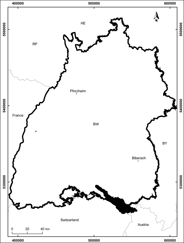
Two study sites in south-western Germany with different topography and species composition (Figure 1) were available. In the study site at Pforzheim (48°52′N, 8°42′E) the topography is steep and hilly. The altitude varies between 260 m and 585 m above sea level. Dominant tree species are beech (Fagus sylvatica L.) and silver fir (Abies alba Mill), which each cover 20% of the area. Scots pine (Pinus sylvestris L.), Norway spruce (Picea abies (L.) Karst.) and douglas fir (Pseudotsuga menziesii (Mirb.) Franco) each cover 15% of the area. The remaining 15% is composed of oak (Quercus rubra and Quercus petrea (Liebl.)) with 8%; Norway maple (Acer platanoides) 3%; ash (Fraxinus excelsior) 2%; and alder and larch (Alnus glutinosa and Larix decidua) each covering 1% of the area [25]. The age of the forest stands ranged between 10 and 200 years. The forest inventory in 2005 indicated that 30% of the trees were smaller than 15 m, 40% were between 15 m and 25 m high, and 30% were higher than 25 m [26].
The topography in the study site at Biberach (48°8′N, 9°43′E) is rather flat with variations in altitude between 500 m and 650 m above sea level. The forest district consists of a temperate coniferous forest dominated by Norway spruce (Picea abies (L.) Karst.), which covers 71% of the area. Other tree species are beech (Fagus sylvatica L.) with 14% and oak (Quercus rubra and Quercus petrea (Liebl.)) with 5%. The remaining 10% of the forest consist of Douglas fir (Pseudotsuga menziesii (Mirb.) Franco), ash (Fraxinus excelsior), Scots pine (Pinus sylvestris L.), silver fir (Abies alba Mill) and larch (Larix decidua); each covering approximately 2% of the area [25]. The age of the forest stands ranged between 10 and 100 years. Tree heights varied between 10 m and 35 m. 10% of the trees were below 15 m high, 40% were between 15 m and 25 m high, 35% between 25 m and 30 m high and 15% were higher than 35 m [27].
In 2005, a forest inventory was conducted in the study site at Pforzheim [26]. The inventory sample plots were arranged in a regular grid of 100 m by 200 m. Each sample plot consisted of three concentric subplots of 12, 6, and 3 m radius, with trees measured at each circular plot depending on threshold diameters at breast height (dbh) of 30, 15, and 10 cm, respectively. This means that trees with a dbh over 30 cm are measured in plots of 12 m radius, trees with dbh between 15 cm and 30 cm are measured in plots of 6 m radius and trees with a dbh below the 15 cm are measured only in a radius of 3 m. Characteristics such as height, dbh and species were measured during the data collection. See [28] for a more precise description of the Baden-Württemberg State Forest sampling protocol that was also followed in the forest inventory used here.
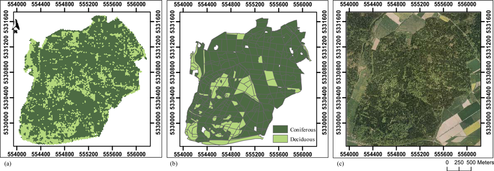
No adequate inventory data was available in the study site at Biberach. Therefore, a grid of plots following the same scheme as the forest inventory in Pforzheim (plots of 12 m radius and spacing of 100 m by 200 m with a random origin) was laid over the study site. The generated plots were classified by visual interpretation of an expert using colour ortho-photographs from 2007 with a spatial resolution of 25 cm.
A total of 365 plots at Pforzheim and 360 plots at Biberach were available as reference for the forest classification. At Pforzheim, the dominant forest type (coniferous or deciduous) for a plot was defined according to the percentage of basal area by deciduous or coniferous species per hectare recorded during the forest inventory in the field. A threshold of 50% was used to decide whether a plot was dominated by deciduous or coniferous trees. In addition, official forest stands maps from 2006 and 2007 were used as visual reference information to evaluate the predictions obtained with the algorithms proposed for the classification of the forest areas. These maps contain information about the percentage of coverage by species per stand based on field estimations [25].

3. Remote Sensing Data

High Resolution SpotLight mode (HS) TerraSAR-X data with an extent of 5 by 10 km were acquired by the German Aerospace Centre (DLR) for the two study sites in 2008 and 2009. The images were provided as Single Look Slant Range Complex (SSC) products [29]. The images were delivered using science orbit information for high accuracy preprocessing [24]. Details regarding each data set are given in Table 1. In this study, only images in HH polarization were analysed.
Weather recordings were acquired seven days before and during the data acquisitions from the weather stations Pforzheim-Ispringen [30] and Augustenberg [31]. These are the two weather stations located closest to the respective study sites. The station in Pforzheim reported a total of 15 mm rainfall before each acquisition (25.07.2008 and 13.03.2009), while the measured rainfall in Biberach was 45 mm between 24.03.2009 and 31.03.2009 and 5 mm between 02.08.2009 and 09.08.2009. Mean temperature in Pforzheim was 5 °C and 16 °C in March and July respectively, while in Biberach it was 4 °C and 18 °C respectively.
Three DEMs were used for the preprocessing of the SAR data: the SRTM DEM Version 4, with spatial resolution of 3 arc seconds (approximately 90 m ground resolution), with WGS84 as the horizontal and EGM96 as the vertical datum [32]; as well as DTMs and DSMs derived from ALS data, with resolution of 5 m, UTM coordinates and DHHN92 vertical datum [33]. In the DHHN92 system the heights were calculated as normal heights with the normal gravity formula of the Geodetic Reference System 1980 (GRS 80) in the level of the NAP [34]. The ALS data was collected in winter 2001 and 2002 for the Laser Scanning DTM Project of Baden-Württemberg [33] with an approximate point density of 0.5 m−s2. This data was provided by the Land and Survey bureau of Baden-Württemberg (LGL). DTMs were computed from the ALS last returns and DSMs from the ALS first returns using the software TreesVis [35].

4. Methods

4.1. Preprocessing of SAR Data

Firstly, an absolute calibration of the backscattered complex signal was carried out applying the constant factor (κ) delivered with the data, which is equivalent to computing the radar brightness (β0) that represents the radar reflectivity per unit area in slant range and is obtained by [36]:
β 0 = κ | i 2 + q 2 |
where i and q represent the imaginary and real parts of the images, respectively.
High Resolution SpotLight mode data provides looks of an image from different viewing angles. As a result, a multilooking technique was used to enhance the quality of the images, by reducing the variability of the individual pixel values induced by non-coherent averaging of the multiple, statistically independent looks [37]. This procedure considers the different looks of the image as multiple independent images that are averaged to obtain a new image called multi-look image. The multilooking in range and azimuth direction depends on the SAR scene and the desired pixel size. As a result, images with lower spatial resolution than the original scene but less radar speckle were obtained. In order to preserve the highest amount of radiometric information as possible but reducing considerably the radar speckle, we decided to produce images in 5 m pixel size, applying multilooking factors between 2 and 4 depending on the scene.
The multi-looked SAR images were orthorectified using the selected DEMs in their original horizontal and vertical datums. However, the SRTM DEM had to be oversampled to 5 m applying a “sinc interpolation” algorithm [38]. The orthorectification of the SAR images was based on a look-up table containing the transformation between the radar and the map geometry [39]. The look-up table was derived from orbital information and elevation of the DEMs, and was refined for more precision by estimating offsets between the SAR image and a simulated SAR image derived from the DEM as reference [40]. The simulated SAR image was transformed to radar geometry and the two images were subsequently divided into small parts, which in turn compared using a cross-correlation algorithm to identify the offsets. A linear polynomial derived from the identified offsets was applied to refine the look-up table. The SAR image was finally transformed to map geometry using the refined look-up table. The map projection of the orthorectified images was UTM zone 32N.
To correct the effects of the incidence angle as well as to eliminate topographic effects, the SAR data were radiometrically calibrated and topographically normalized by calculating sigma naught (σ0) and gamma naught (γ0) images [41]. Given the local incidence angle, the scattering coefficients are obtained by:
σ 0 = β 0 sin ( Θ loc )
γ 0 = σ 0 cos ( Θ loc )
where Θloc is the local incidence angle, β0 constitutes the radar brightness, σ0 represents the radar reflectivity per unit area in ground range assuming a flat terrain and γ0 is the fully terrain corrected reflectivity.
The average and standard deviation of the scattering coefficients within each sample plot were used as explanatory variables for statistical modeling. The data preprocessing, with the DEMs derived from ALS data (ALS DEMs), was carried out in the GAMMA software suite [42], which supports the original coordinate system of the ALS DEMs. Preprocessing with the SRTM was carried out with the open source Next ESA SAR Toolbox (4B) [38], which especially supports the orthorectification with SRTM and provides more accurate algorithms for its resampling.

4.2. Data Analysis

The primary focus of the data analysis was the classification of deciduous- and coniferous-dominated forest using TerraSAR-X images preprocessed with different DEMs. However, considering the fact that the level of accuracy of the pixel location influences the successful linking of ground truth reference data and the remote sensing data, the first step of the analysis was an exploratory evaluation of the pixel location accuracy of orthorectified images.

4.2.1. Location Accuracy of Orthorectified SAR Data

The analysis of the pixel location accuracy was based on the comparison of coordinates of 35 reference points identifiable in the SAR images as well as in an official digital topographic map in scale 1:25,000. The reference map was available in raster format with a location accuracy of about 1.5 m. The reference map is based on orthophotos from 2007 scale 1:10,000 [43].
Most of the reference points were located at road crossings. The accuracy was assessed based on the root mean squared error (RMSE). The grainy appearance of the SAR images [21] complicated the detection of the reference points on fine display scales. Therefore, they were digitized using display scales between 1:3,500 and 1:4,500. On these display scales we did not identify single pixels, but a small area in the image. In addition to the identification of the 35 reference points, forest stands were delineated using each of the orthorectified images and their borders were compared using the digital topographic map.

4.2.2. Classification of Coniferous- and Deciduous-Dominated Forest

The binary response variable y (plot dominated by conifers or deciduous trees) was modelled using a generalized linear model (GLM). The GLM is an extension of the linear model that allows fitting data with a binomial probability distribution [44]. For a detailed description of GLMs see [45].
If g denotes the logarithm as a link function, then the logistic regression equation can be denoted as
π i = exp ( η i ) 1 + exp ( η i ) ; η i = x i β , i = 1 , , n
where πi is the probability of the ith element constituting a member of one of the two classes (coniferous- or deciduous-dominated) and ηi is a linear predictor, with xi representing a vector of independent variables and β the vector of regression parameters.
An automatic stepwise procedure with forward and backward selection based on the analysis of variance was used to select the most relevant variables in the GLM [44].
Several criteria were taken into consideration to compare the quality of models based on the differently preprocessed images: (a) producer’s accuracy (PA), user’s accuracy (UA) and overall accuracy (OA); (b) Cohen’s Kappa coefficient (κ); and (c) the Bayesian information criterion (BIC). The BIC criterion entails the number of parameters and therefore tends to penalize the overly complex models [46]. The categories proposed by Landis and Koch [47] were used to interpret the kappa coefficients: κ < 0.20 poor, 0.21 < κ ≤ 0.40 fair, 0.41< κ ≤ 0.60 moderate, 0.61 < κ ≤ 0.80 good, 0.81 < κ ≤ 1 very good. Statistical analysis was carried out in the R software for statistical computing [48]. All reported accuracy criteria were based on a leave-one-out cross-validation method (e.g., [49]) to avoid overfitting.
Finally, to test the application of the algorithms on large areas, we generated prediction maps of coniferous- and deciduous-dominated forest stands using the best models. For this purpose, forest areas of the study sites were divided into hexagons with the same size of the reference sample plots (452 m2). The values of the explanatory variables were extracted for each hexagon and were used to predict its forest class. Predictions were displayed in map form and visually compared with the official forest stands map and the colour orthophotos, both from 2007.

5. Results

5.1. Location Accuracy of Orthorectified SAR Data

The analysis of stand borders in Figure 2 revealed shifts up to 7 pixels (35 m) in images orthorectified with the SRTM compared with the reference map. However, the lower left hand corner of the border and in general the position of the lower border was very accurate, which shows that shifts were not the same in all directions. The stand boundaries between images orthorectified with the ALS DEMs were very similar. The differences regarding the reference map were between 1 and 5 pixels (5 to 25 m). In Pforzheim, leaf-off and leaf-on images orthorectified with the ALS DSM did not have the same position accuracy. The leaf-off image was more accurate than the leaf-on image (approximately 1 pixel difference).
The evaluation of the position accuracy with the 35 selected points is shown in Table 2. Reference coordinates were taken from the official digital topographic map (scale 1:25,000). The reported values are only an approximation of the true error, because digitalization also lacks precision due to the fact that the reference points are hard to detect in the SAR images. The fact that inaccurate pixel locations can lead to incorrect classification of reference plots can be observed in Figure 3. In some cases, the same sample plot is located in different land use classes depending on the DEM used for orthorectification.

5.2. Classification of Coniferous- and Deciduous-Dominated Forest

In general, γ0 images resulted in lower classification accuracies compared with σ0 images. Only in Pforzheim γ0 images obtained with the ALS DTM delivered higher classification accuracy than the σ0 image, although the differences were not large (approximately 1%). Therefore, only results based on σ0 images will be presented in the following.
Variable selection indicated that only the mean of the SAR backscatter (σ0) on a sample plot is significant for the distinction of forest types (Figure 4). Plots dominated by coniferous trees tended to have lower σ0 values than plots dominated by deciduous trees.
Leaf-off images were more accurate for the classification of deciduous- or coniferous-dominated forest than leaf-on images (Table 3). We observed a seasonal variation in backscatter values between plots dominated by coniferous or deciduous trees. For example, in Pforzheim, the analysis of σ0 images preprocessed with ALS DEMs revealed that the average SAR backscatter in plots dominated by coniferous trees increased between 0.4 dB and 0.8 dB from July 2008 to March 2009; while in plots dominated by deciduous trees the increase was from 1.6 dB to 1.7 dB. Similar tendencies were also observed in Biberach.
In both study sites, the combination of leaf-off and leaf-on images preprocessed with the ALS DTMs improved the classification considerably (Table 3), resulting in an overall accuracy of 78.3% in Biberach and 71.2% in Pforzheim (Appendix 1). This was also the case for the images preprocessed with the ALS DSM in Biberach. In Pforzheim, the combination of leaf-off and leaf-on images preprocessed with the ALS DSM did not improve the classification accuracy compared to using leaf-off images only. The covariates in the logistic regression were the mean of the SAR backscatter in summer and winter as well as their interaction (Appendix 2). The interaction term represents the differences in the seasonal variation of the SAR backscatter between plots dominated by coniferous or deciduous trees. Figure 5 shows the results of forest classification in Biberach by combining leaf-on and leaf-off images preprocessed with the ALS DTM.

6. Discussion

The aim of this study was to map coniferous- and deciduous-dominated forest based on TerraSAR-X images from different seasons. For the supervised classification approach followed, high pixel location accuracy is mandatory. In order to obtain high pixel position accuracy, an accurate orbit determination and high quality DEM are necessary [50]. SAR data for this study was acquired in science orbit with errors <50 cm [24]. Therefore, although the applied preprocessing chain can influence the orthorectification of the data [
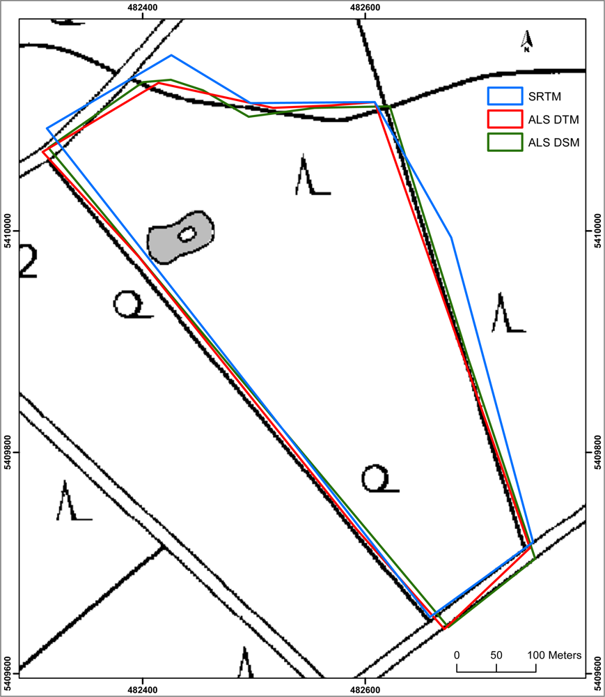
51], we assume that the observed displacement errors resulted mostly from the vertical error of the DEMs. For example, a vertical error of 1 m meant a ground range displacement of approximately 1.5 m in the orthorectified images for the acquired SAR data.
Due to the difficulty of identifying reference points within the forest in both the SAR images and the reference map, the position error of the images was measured based on man-made objects. Although we assumed that the orthorectification with the DSM should generate higher precision in forest areas, we were not able to confirm significant differences between images orthorectified with ALS DSMs and ALS DTMs. A factor that must be considered especially for SAR images in leaf-off conditions, is that the radar backscatter of deciduous forest was also scattered from points below the top of the trees (e.g., [4,52,53]). This is not reflected by the DSM. Another reason for inaccurate orthorectification with the DSM, both in leaf-off and leaf-on conditions, could be that the forest structure has changed due to the time difference between the acquisitions of the ALS and SAR data. Thus, the ALS DSM did not exactly represent the canopy structure during SAR data acquisition.
Holopainen et al. [20] evaluated the location accuracy of TerraSAR-X images orthorectified with a national DEM (25 m resolution). They report an average accuracy of 4 m which is comparable to the accuracy we obtained with the ALS DEMs. However, small errors of 1 or 2 pixels (equivalent to 10 m) in the position of the reference points can also be attributed to digitization errors and not necessarily to the orthorectification of the SAR images, because coarse display scales have been used to identify the reference points in the SAR images. Since we focussed on the classification of SAR images, only the relative difference in location accuracy between SAR images that were orthorectified with different DEMs was of interest. An appropriate analysis of the pixel location accuracy can only be achieved with good ground references, for example using corner reflectors (CR) at the time of acquisition. A geolocation accuracy of TerraSAR-X images superior to 1 m can then be observed [50,54].
σ0 and γ0 images were calculated to eliminate the effect of the local terrain undulations. The accuracy of σ0 and γ0 scattering coefficients depend on the spatial resolution of the DEM used for the calibration. A high spatial resolution allows the calculation of the local scattering area to be more accurate and to identify shadow and layover regions correctly [55]. Because the study site of Biberach was rather flat, we did not identify a significant difference between σ0 and γ0 scattering coefficients obtained with the ALS DTM. In Pforzheim, the topographic normalization (γ0) using the ALS DTM effected the local backscattering of areas with high terrain slopes. However, the difference of the classification accuracy based on σ0 and γ0 images was small in Pforzheim because only few inventory sample plots were located on steep slopes. The topographic normalization with ALS DSMs resulted in a large number of shadow pixels in the γ0 images. Therefore, σ0 images were more suitable than γ0 images if the topographic normalization was based on ALS DSMs in both study areas.
The analysis of the statistical criteria indicated that images preprocessed with the SRTM were not satisfactory for the classification of coniferous- and deciduous-dominated forest as consequence of the low spatial resolution of the SRTM DEM. The best model for the classification was obtained by combining leaf-off and leaf-on images preprocessed with ALS DTMs. While the improved accuracy by combining leaf-off and leaf-on images preprocessed with the ALS DSM was also visible in Biberach, this was not the case in Pforzheim. The reason was a less accurate orthorectification of the leaf-on image with the ALS DSM.
Pierce et al. [56] used the mean and standard deviation of the radar backscatter (σ0) to discriminate land cover classes in Michigan. As in our study, they also observed lower backscatter values for coniferous than for deciduous forests in X-band SAR images [18]. A better differentiation between deciduous and coniferous tree types in leaf-off SAR images was found by Hoekman [57]. Furthermore, he reported an improvement of the classification accuracy by combining images from different seasons. Both of his observations were supported by our results. Some explanations for the seasonal variation of the radar backscatter (σ0) were given by Dobson et al. [58]. Midsummer conditions, for example, lead to a decrease of σ0 because of the attenuation of the radar signal caused by the presence of foliage and other elements in the crown, as well as dielectric changes in the trunks and branches.
Rainfall before the image acquisition under leaf-off conditions at the Biberach study site prevents a generalization of the results obtained with this data set, as moisture can have a significant impact on the radar backscatter [59]. This can even lead to more accurate classification results. Changes in the radar backscatter after rain depend on the land use and forest type [6063]. For example, the effect of rainwater on the radar backscatter tends to be larger for deciduous than for coniferous forests [63].
The differences between the Biberach and Pforzheim reference datasets contributed to the difference in the classification accuracy in the two study sites. The visual classification of the reference plots using orthophotographs in Biberach was better related to the SAR backscatter, because in both remote sensing sources only the upper dominant canopy layer contributes to the reflection. The proportion of basal area measured in the field, which was used as reference in Pforzheim, also included trees from the understory, which may not have contributed to the SAR backscatter. In comparison to Hoekman [57] and Rignot et al. [12], the accuracy achieved in our study was low. However, they classified monospecies homogeneous stands in a coarser scale of mapping (stand level), whereas we dealt with heterogeneous mixed forest and minimum mapping units of 450 m2. Breidenbach et al. [18] observed that classification accuracy reduced considerably with a decreasing minimum mapping unit.

7. Conclusion

The use of High Resolution SpotLight TerraSAR-X (SAR) images in HH-polarization allowed the classification of coniferous- and deciduous-dominated forest with fair to moderate accuracy. The use of high resolution digital elevation models (DEMs) for orthorectification of the SAR images was found to be important to achieve greater pixel location accuracy. The orthorectification and the radiometric calibration influenced the classification accuracy of coniferous- and deciduous-dominated forest; the accuracy was higher when SAR images were preprocessed with airborne laser scanning (ALS) DEMs than when SAR images were preprocessed with a C-band Shuttle Radar Topography Mission (SRTM) DEM.
Images preprocessed with ALS digital surface models (DSMs) and ALS digital terrain models (DTMs) resulted in similar classification accuracies. Higher orthorectification accuracy and correct calibration, as well as normalization of the radar backscatter in vegetated areas should theoretically be obtained by preprocessing SAR images with a DSM. We were unable to confirm this hypothesis due to the potential influence of the time lag between the ALS and SAR data acquisition on our results.
SAR images acquired under leaf-off conditions resulted in slightly better classification accuracies than SAR images acquired under leaf-on conditions. The classification accuracy was improved through the combination of leaf-off and leaf-on images.
It will be of interest to study whether the theoretical advantage of digital surface models from airborne laser scanning data can be verified when ALS and SAR data are acquired at the same time. Higher pixel location accuracy will gain importance in future studies when objects with higher spatial heterogeneity, such as small groups of trees attacked by bark beetles, need to be identified.

Appendices

Appendix 1. Confusion matrix of leaf-one-out predictions based on combined leaf-off and leaf-on images (σ0) preprocessed with ALS DTMs.
SiteBiberachPforzheim
Reference
PredictionConiferousDeciduousRow totalConiferousDeciduousRow total
Coniferous2104725715557212
Deciduous317210348105153
Column total241119360203162365
Producer’s accuracy (%)87.160.576.464.8
User’s accuracy (%)81.769.973.168.6
Overall accuracy (%)78.371.2
Kappa coefficient (κ)0.490.41

Appendix 2. Parameters of the generalized linear models for the classification of deciduous and coniferous forest with the highest accuracy.
BiberachPforzheim
EstimateStd. Errorp-valueEstimateStd. Errorp-value
Intercept1.316.280.8321.64.36<0.01
σ0 leaf-off (mean)−0.350.430.421.460.32<0.01
σ0 leaf-on (mean)−0.610.440.171.170.28<0.01
leaf-off * leaf-on (mean)−0.070.030.010.070.02<0.01
Figure 1. Location of study sites Pforzheim and Biberach in UTM coordinate system (zone 32N) with the surrounding countries and federal states (BW = Baden-Württemberg, BY = Bavaria, HE = Hesse, RP = Rhineland-Palatinate).
Remotesensing 04 00661f1
Figure 2. Boundary of a forest stand located in Pforzheim, digitized from three different orthorectified TerraSAR-X images in leaf-off conditions. The official digital topographic map is shown as reference in UTM coordinates (zone 32N).
Remotesensing 04 00661f2
Figure 3. Example of orthorectified images of Pforzheim in leaf-off conditions (left) and DEMs used for the orthorectification (right). Inventory plots are shown as red circles. The big blue circle highlights a sample plot that was located in another land use class in the image orthorectified with the SRTM (UTM coordinates of zone 32N are displayed in the image margins.).
Remotesensing 04 00661f3
Figure 4. Boxplots of SAR backscatter (σ0) on sample plots dominated by coniferous or deciduous trees in images preprocessed with ALS DSMs. (a) Leaf-off images and (b) Leaf-on images.
Remotesensing 04 00661f4
Figure 5. Application of the classification model in Biberach. (a) Map of deciduous- and coniferous-dominated forest based on combined leaf-on and leaf-off TerraSAR-X images (acquired in 2008 and 2009) preprocessed with the ALS DTM; (b) official forest stand map (established 2007); (c) ortho-photographs (acquired on 2007).
Remotesensing 04 00661f5
Table 1. Properties of High Resolution SpotLight (HS) TerraSAR-X datasets.
BiberachPforzheim
Date27.03.200909.08.200925.07.200813.03.2009
Time17:08:2605:34:5505:43:1905:43:19
PolarizationHH and VVHHHHHH
Orbital directionAscendingDescendingDescendingDescending
Mean and range of incidence angles (°)39.3 (38.9–39.8)37.5 (37–37.9)31.7 (31.1–32.2)31.7 (31.1–32.2)
Slant range resolution (m)1.171.171.171.17
Projected spacing azimuth (m)1.810.860.860.88
Table 2. Location accuracy of leaf-off synthetic aperture radar (SAR) images orthorectified with three different digital elevation models (DEM)s.
DEMRMSE (m)
BiberachPforzheim
xyEuclidian DistancexyEuclidian Distance
ALS DSM9711759
ALS DTM10712647
SRTM DEM15101529825
Table 3. Classification accuracy of deciduous- and coniferous-dominated sample plots using leaf-off and leaf-on SAR images (σ0).
BiberachPforzheim
OA (%)κκ conf. int. (level = 0.95)OA (%)κκ conf. int. (level = 0.95)
Leaf-off

ALS DTM71.10.250.13–0.3867.90.340.25–0.44
ALS DSM70.80.250.13–0.3768.50.350.26–0.45
SRTM67.80.150.02–0.2766.60.320.21–0.42

Leaf-on

ALS DTM70.00.180.05–0.3164.10.260.16–0.36
ALS DSM70.00.220.09–0.3460.50.180.07–0.28
SRTM66.90.01(−0.1) −0.1658.10.09(−0.1) −0.20

Combination of leaf-off and leaf-on

ALS DTM78.30.490.38–0.5871.20.410.32–0.51
ALS DSM76.10.440.35–0.5568.20.350.25–0.45
SRTM70.00.230.11–0.3566.60.320.21–0.42

Acknowledgments

We would like to thank Barbara Koch, Department of Remote Sensing and Landscape Information Systems of the University of Freiburg, for her cooperation in the “Insect Combat” and “FoX” projects, as well as Christiane Schmullius, Department of Earth Observation at the University of Jena for support in the preprocessing of the SAR data. We acknowledge the provision of TerraSAR-X data by the German Aerospace Center (DLR) within the Forest monitoring with TerraSAR-X (FoX) project. This research was partially financed by the European Space Agency (ESRIN/AO/1-5781/08/I-EC).

References

  1. Lindner, M.; Maroschek, M.; Netherer, S.; Kremer, A.; Barbati, A.; Garcia-Gonzalo, J.; Seidl, R.; Delzon, S.; Corona, P.; Kolström, M.; et al. Climate change impacts, adaptive capacity, and vulnerability of European forest ecosystems. Forest Ecol. Manage 2010, 259, 698–709. [Google Scholar]
  2. Deshayes, M.; Guyon, D.; Jean, H.; Stach, N.; Jolly, A.; Hagolle, O. The contribution of remote sensing to the assessment of drought effects in forest ecosystems. Ann. For. Sci 2006, 63, 579–595. [Google Scholar]
  3. Ciesla, W. Remote Sensing in Forest Health Protection; FHTET Report No. 00-03; USDA Forest service, Remote sensing Applications Center Salt Lake City, UT and Forest Health Technology Enterprise Team: Fort Collins, CO, USA, 2000; pp. 197–211. [Google Scholar]
  4. Perko, R.; Raggam, H.; Deutsche, J.; Gutjahr, K.; Schardt, M. Forest assessment using high resolution SAR data in X-band. Remote Sens 2011, 3, 792–815. [Google Scholar]
  5. Wulder, M.; White, J.; Coops, N.; Han, T.; Alvarez, M.; Butson, C.; Yuan, X. A Procedure for Mapping and Monitoring Mountain Pine Beetle Red Attack Forest Damage Using Landsat Imagery. BC-X-404; Information Report, Pacific Forestry Centre. 2006, pp. 1–40. http://www.for.gov.bc.ca/hfd/library/documents/bib96701.pdf (accessed on 17 January 2011).
  6. Ranson, K.; Kovacs, K.; Sun, G.; Kharuk, V. Disturbance recognition in the boreal forest using radar and Landsat-7. Can. J. Remote Sens 2003, 29, 271–285. [Google Scholar]
  7. Knowlton, D.; Hoffer, R. Radar Imagery for Forest Cover Mapping. Proceedings of the 7th International Symposium on Machine Processing of Remotely Sensed Data, West Lafayette, IN, USA, 23–26 June 1981; pp. 626–632.
  8. Leckie, D.; Ranson, K.J. Forestry Applications Using Imaging Radar. In Principles and Applications of Imaging Radar (Manual of Remote Sensing), 3rd ed.; Henderson, F., Lewis, A., Eds.; John Wiley & Sons Inc: New York, NY, USA, 1998; pp. 435–509. [Google Scholar]
  9. Thiel, C.; Santoro, M.; Cartus, O.; Thiel, C.; Riedel, T.; Schmullius, C. Perspectives of SAR based Forest Cover, Forest Cover Change and Biomass Mapping. In The Kyoto Protocol: Economic Assessments, Implementation Mechanisms, and Policy Implications; Vasser, C.P., Ed.; Nova Science Publishers Inc: Hauppauge, NY, USA, 2009; pp. 13–56. [Google Scholar]
  10. Churchill, P.; Keech, M. SAR Investigations of Thetford Forest. JRC/ESA SAR 580 Investigators Final Workshop, Ispra, Italy, 15–17 May 1984; pp. 533–550.
  11. Leckie, D. Synergism of SAR and visible/infrared data for forest type discrimination. Photogramm. Eng. Remote Sensing 1990, 56, 1237–1246. [Google Scholar]
  12. Rignot, E.; Williams, C.; Way, J.; Viereck, L. Mapping of forest types in Alaskan boreal forest using SAR imagery. IEEE Trans. Geoci. Remote Sens 1994, 32, 1051–1059. [Google Scholar]
  13. Dobson, M.; Ulaby, F.; Pierce, L. Land-cover classification and estimation of terrain attributes using synthetic aperture radar. Remote Sens. Environ 1995, 51, 199–214. [Google Scholar]
  14. Saatchi, S.; Rignot, E. Classification of boreal forest cover types using SAR images. Remote Sens. Environ 1997, 60, 270–281. [Google Scholar]
  15. Koch, B. Status and future of laser scanning, synthetic aperture radar and hyperspectral remote sensing data for forest biomass assessment. ISPRS J. Photogramm 2010, 65, 581–590. [Google Scholar]
  16. Roth, A.; Eineder, M.; Schättler, B. TerraSAR-X: A New Perspective for Applications Requiring High Resolution Spaceborne SAR Data. Proceedings of the Joint ISPRS 6 EarSel Workshop on High Resolution Mapping from Space 2003, Hannover, Germany, 6–8 October 2003; pp. 1–4.
  17. Düring, R.; Koudogbo, F.; Weber, M. TerraSAR-X and TanDEM-X: Revolution in Spaceborne Radar. Int. Arch. Photogramm. Remote Sens. Spat. Inf. Sci. 2008, XXXVII. http://www.isprs.org/proceedings/XXXVII/congress/1_pdf/37.pdf (accessed 17, January 2011).
  18. Breidenbach, J.; Ortiz, S.; Reich, M. Forest monitoring with TerraSAR-X: first results. Eur. J. For. Res 2010, 129, 813–823. [Google Scholar]
  19. Karjalainen, M.; Kankare, V.; Vastaranta, M.; Holopainen, M.; Hyyppä, J. Prediction of plot-level forest variables using TerraSAR-X stereo SAR data. Remote Sens. Environ 2011. [Google Scholar] [CrossRef]
  20. Holopainen, M.; Haapanen, R.; Karjalainen, M.; Vastaranta, M.; Hyyppä, J.; Yu, X.; Tuominen, S.; Hyyppä, H. Comparing accuracy of airborne laser scanning and TerraSAR-X radar images in the estimation of plot-level forest variables. Remote Sens 2010, 2, 432–445. [Google Scholar]
  21. Oliver, C.; Quegan, S. Understanding Synthetic Aperture Radar Images; SciTech Publishing, Inc.: Boston, MA, USA, 2004; pp. 43–72. [Google Scholar]
  22. Beaudoin, A.; Stussi, N.; Troufleau, D.; Desbois, N.; Piet, L.; Deshayes, M. On the Use of ERS-1 SAR Data over Hilly Terrain: Necessity of Radiometric Corrections for Thematic Applications. Proceedings of 1995 International IEEE Geoscience and Remote Sensing Symposium, Firenze, Italy, 10–14 July 1995; 3, pp. 2179–2182.
  23. Saundercock, G. The geocoding of synthetic aperture radar imagery and an application to nautical charting. Photogramm. Rec 1995, 15, 57–64. [Google Scholar]
  24. Koppe, W.; Kiefl, N.; Hennig, S.; Janoth, J. Validation of Pixel Location Accuracy of Orthorectified TerraSAR-X Products. EUSAR 2010, Aachen, Germany, 7–10 June 2010; pp. 106–108.
  25. FoGIS-InFoGIS (Forestry Geographic Information System). Available online: http://www.disy.net/referenzen-alt/referenzen-fachgebiet/raeumliche-planung/infogis.html (accessed on 17 January 2011).
  26. Forst BW (Forest Service of Baden-Württemberg). Forest Inventory in the Forest District of Pforzheim. Internal Digital Database. 2005. Available online: http://www.forstbw.de/landesbetrieb-forstbw/schuetzenbewahren/waldinventuren/forsteinrichtung/ (accessed on 17 January 2011).
  27. Forst BW (Forest Service of Baden-Württemberg). Forest Inventory in the Forest District of Biberach. Internal Digital Database. 2003. Available online: http://www.forstbw.de/landesbetrieb-forstbw/schuetzenbewahren/waldinventuren/forsteinrichtung/ (accessed on 17 January 2011).
  28. Breidenbach, J.; Nothdurft, A.; Kändler, G. Comparison of nearest neighbour approaches for small area estimation of tree species-specific forest inventory attributes in central Europe using airborne laser scanner data. Eur. J. For. Res 2010, 129, 833–846. [Google Scholar]
  29. DLR (Deutsches Zentrum für Luft und Raumfahrt), TerraSAR-X, Ground Segment, Basic Products Specification Document; DLR: Oberpfaffenhofen, Germany, 2006; pp. 1–45.
  30. DWD. Deutscher Wetterdienst. WESTE (Wetterdaten und-Statistiken Express)-Allgemein. 2009. Available online: http://www.dwd-shop.de/details/1122d.html (accessed on 17 January 2011).
  31. LTZ. Landwirtschaftliches Technologiezentrum Augustenberg. Wetterdaten-Infoservice Pflanzenbau & Pflanzenschutz. 2009. Available online: http://www.wetterbw.de/wetterdaten/tabelle/tageswerte/index.php?Stations_ID=99&Jahr=2009&Anzeigen=OK (accessed on 17 January 2011).
  32. Jarvis, A.; Reuter, H.I.; Nelson, A.; Guevara, E. Hole-Filled SRTM for the Globe Version 4. CGIAR-CSI SRTM 90m Database. 2008. Available online: http://srtm.csi.cgiar.org (accessed on 17 January 2011).
  33. Schleyer, A. Das Laserscan-DGM von Baden-Württemberg. In Photogrammetric Week 01; Fritsch, D., Spiller, R., Eds.; Wichmann: Heidelberg, Germany, 2001; pp. 217–225. [Google Scholar]
  34. Ihde, J.; Habrich, H.; Hornik, H.; Pahle, K.; Schlüter, W. Precise Positioning on Global and Regional Scales, National Report of the Federal Republic of Germany on the Geodetic Activities in the years 1999–2003. 2003; 11–19.
  35. Weinacker, H.; Koch, B.; Weinacker, R. TREESVIS: A Software System for Simultaneous ED-Real-Time Visualisation of DTM, DSM, Laser Raw Data, Multispectral Data, Simple Tree and Building Models. Proceedings of the ISPRS Working Group VIII (2), Freiburg, Germany, October 2004; pp. 90–95.
  36. Raney, K. Radar Fundamentals: Technical Perspective. In Principles and Applications of Imaging Radar (Manual of Remote Sensing), 3rd ed.; Henderson, F., Lewis, A., Eds.; John Wiley & Sons Inc: New York, NY, USA, 1998; pp. 32–45. [Google Scholar]
  37. Ranney, K.; Tran, C. Effects of registration error on multi-look averaged data. Proc. SPIE 2005, 5794, 447–458. [Google Scholar]
  38. ESA. Array Systems Computing Inc. NEST User Manual. Available online: http://nest.s3.amazonaws.com/docs/nest_user_manual-4B.pdf (accessed on 27 January 2012).
  39. Wegmüller, U. Automated Terrain Corrected SAR Geocoding. Proceedings of International Geoscience and Remote Sensing Symposium (IGARSS ’99), Hamburg, Germany, 28 June–2 July 1999; pp. 1712–1714.
  40. Santoro, M.; Fransson, J.; Erikkson, L.; Magnusson, M.; Ulander, L.; Olsson, H. Signatures of ALOS PALSAR L-Band backscatter in Swedish forest. IEEE Trans. Geosci. Remote Sens 2009, 47, 4001–4019. [Google Scholar]
  41. Stussi, N.; Beaudoi, A.; Castel, T.; Gigord, P. Radiometric Correction of Multi-Configuration Space-borne SAR Data over Hilly Terrain. Proceedings of International Symposium on Retrieval of Bio- and Geophysical Parameters from SAR Data for Land Applications, Toulouse, France, 10–13 October 1995; pp. 469–478.
  42. Wegmüller, U.; Werner, C.; Strozzi, T.; Wiesmann, A.; Santoro, M. Gamma SAR and Interferometry Software; Gamma AG: Bern, Switzerland, 2006. [Google Scholar]
  43. ATKIS (Amtliche Topographisch-Kartographische Informationssystem). Official Map 1:25000. Available online: http://www.lv-bw.de/lvshop2/start_ie.asp?openkey=PRODUKTE&keyinfo=&os=Win32&mapw=600 (accessed on 13 January 2012).
  44. Venables, W.; Ripley, B. Modern Applied Statistics with S. Statistics and Computing, 4th ed.; Springer: New York, NY, USA, 2002; pp. 183–208. [Google Scholar]
  45. McCullagh, P.; Nelder, J. Generalized Linear Models, 2nd ed.; Chapman & Hall: London, UK, 1989. [Google Scholar]
  46. Trevor, H.; Tibshirani, R.; Friedman, J. The Elements of Statistical Learning, Data Mining, Inference, and Prediction, 2nd ed.; Springer: New York, NY, USA; p. 2009.
  47. Landis, J.; Koch, G. The measurement of observer agreement for categorical data. Biometrics 1977, 33, 159–174. [Google Scholar]
  48. R (Development Core Team). R a Language and Environment for Statistical Compution. 2010. Available online: http://cran.r-project.org/doc/manuals/refman.pdf (accessed on 17 January 2011).
  49. Golub, G.; Heath, M.; Wahba, G. Generalised cross-validation as a method for choosing a good ridge parameter. Technometrics 1979, 21, 215–223. [Google Scholar]
  50. Nonaka, T.; Ishizuka, Y.; Yamane, N.; Shibayama, T.; Takagishi, S.; Sasagawa, T. Evaluation of the geometric accuracy of TerraSAR-X. Int. Arch. Photogramm. Remote Sens. Spat. Inf. Sci 2008, XXXVII(B7), 135–140. [Google Scholar]
  51. Werner, C.; Strozzi, T.; Wegmüler, U.; Wiesmann, A. SAR Geocoding and Multi-Sensor Image Registration. Proceedings of 2002 IEEE International Geoscience and Remote Sensing Symposium, Toronto, ON, Canada, 24–28 June 2002; 2, pp. 902–904.
  52. Kobayashi, Y.; Sarabandi, K.; Pierce, L.; Dobson, M. An evaluation of the JPL TOPSAR for extracting tree heights. IEEE Trans. Geosci. Remote Sens 2000, 38, 2446–2454. [Google Scholar]
  53. Izzawati, I.; Wallington, E.; Woodhouse, I. Forest height retrieval from commercial X-band SAR products. IEEE Trans. Geosci. Remote Sens 2006, 44, 863–870. [Google Scholar]
  54. Fritz, T.; Breit, H.; Eineder, M. TerraSAR-X Products Tips and Tricks. Proceedings of 3rd TerraSAR-X Workshop, Oberpfaffenhofen, Germany, 26 November 2008.
  55. Loew, A.; Mauser, W. Generation of geometrically and radiometrically terrain corrected SAR image products. Remote Sens. Environ 2007, 106, 337–349. [Google Scholar]
  56. Pierce, L.; Bergen, K.; Dobson, M.; Ulaby, F. Multitemporal land-cover classification using SIR-C/X-SAR imagery. Remote Sens. Environ 1997, 64, 20–23. [Google Scholar]
  57. Hoekman, D. Radar backscatter of forest stands. Int. J. Remote Sens 1985, 6, 325–343. [Google Scholar]
  58. Dobson, M.; Pierce, L.; McDonald, K.; Sharik, T. Seasonal Change in Radar Backscatter from Mixed Conifer and Hardwood Forest in Northern Michigan. Proceedings of International Geoscience and Remote Sensing Symposium (IGARSS ’91), Helsinki, Finland, June 1991; pp. 1121–1124.
  59. Ulaby, F.; Brisco, B.; Dobson, C. Improved spatial mapping of rainfall events with spaceborne SAR imagery. IEEE Trans. Geosci. Remote Sens 1983, 21, 118–121. [Google Scholar]
  60. Fischer, J.; Brown, R.; Brisco, B. The Effects of Changes in Soil Moisture and Rainfall on SAR Data Crop Classification. Proceedings of Fifteenth Canadian Symposium of Remote Sensing, Toronto, ON, Canada, 1–4 June 1992; pp. 221–226.
  61. Gillespie, T.; Brisco, B.; Brown, R.; Sofko, G. Radar detection of a dew event in wheat. Remote Sens. Environ 1990, 33, 151–156. [Google Scholar]
  62. Rignot, E.; Way, J.; McDonald, K.; Viereck, L.; Williams, C.; Adams, C.; Wood, W.; Shi, J. Monitoring of environmental conditions in Taiga forest using ERS-1 SAR. Remote Sens. Environ 1994, 49, 145–154. [Google Scholar]
  63. De Jong, J.; Klaassen, W.; Kuiper, P. Monitoring of rain water storage in forest with satellite radar. IEEE Trans. Geosci. Remote Sens 2002, 40, 338–347. [Google Scholar]

