Simulating Forest Cover Changes of Bannerghatta National Park Based on a CA-Markov Model: A Remote Sensing Approach

Department of Geography, Land-Use and Environmental Change Institute, University of Florida, 3141 Turlington Hall, Gainesville, FL 32611, USA
*
Author to whom correspondence should be addressed.
Remote Sens. 2012, 4(10), 3215-3243; https://0-doi-org.brum.beds.ac.uk/10.3390/rs4103215
Submission received: 9 August 2012
/
Revised: 5 October 2012
/
Accepted: 12 October 2012
/
Published: 22 October 2012
Abstract
:Establishment of protected areas (PA) has been one of the leading tools in biodiversity conservation. Globally, these kinds of conservation interventions have given rise to an increase in PAs as well as the need to empirically evaluate the impact of these PAs on forest cover. Few of these empirical evaluations have been geared towards comparison of pre and post policy intervention landscapes. This paper provides a method to empirically evaluate such pre and post policy interventions by using a cellular automata-Markov model. This method is tested using remotely sensed data of Bannerghatta National park (BNP) and its surrounding, which have experienced various national level policy interventions (Indian National Forest Policy of 1988) and rapid land cover change between 1973 and 2007. The model constructs a hypothetical land cover scenario of BNP and its surroundings (1999 and 2007) in the absence of any policy intervention, when in reality there has been a significant potential policy intervention effect. The models predicted a decline in native forest cover and an increase in non forest cover post 1992 whereas the actual observed landscape experienced the reverse trend where after an initial decline from 1973 to 1992, the forest cover in BNP is towards recovery post 1992. Furthermore, the models show a higher deforestation and lower reforestation than the observed deforestation and reforestation patterns for BNP post 1992. Our results not only show the implication of national level policy changes on forest cover but also show the usefulness of our method in evaluating such conservation efforts.
1. Introduction
Over the last few decades, tropical deforestation has been one of the major changes in terrestrial landscapes affecting the global environment [1–3]. Forest cover decline results in loss of biodiversity, increases the incidences of flooding, soil degradation and influences the climate [4,5]. During the 1990s, the world has lost about 8.3 million hectares of forest per year, and in the period from 2000 to 2010 a reduced, but still significant rate of 5.2 million hectares lost per year (values account for deforestation and afforestation/reforestation to obtain final loss values) [5]. Of this forest cover loss, most occurred in biodiversity rich natural tropical forest areas [3,5]. The Global Forest Resources Assessment (2010) showed that forest covers 31% of the world land area, with over half of this lying in the world’s five richest countries (Russian Federation, Brazil, Canada, USA and China). 64 countries have less than 10% forest cover and of these ten have no forest at all. Globally, protected areas (PAs) still remain the most popular conservation approach to protect biodiversity [6–15]. Often it is assumed that legal protection will bring positive impact on the forest cover of an area and help in lowering deforestation [16]. As a result, total forested area under protection globally has increased from 3.48% in 1985 [17] to 13% in 2010 [5], this represents a 94 million hectare increase since 1990, with two thirds of the increase occurring since 2000 [5]. Legally established protected areas now cover 13% of the world’s forests and 12% of the world’s forests are designated for some form of biological diversity conservation, but not all of the latter occur within the former [5]. Nevertheless, the effectiveness of PAs in maintaining forest cover has been debated and is still questioned [18]. One of the fundamental questions in PA creation is, “how do we know that PAs are effective in maintaining forest cover?” In other words, to understand the impact of a protection, we want to know what would have happened to forest cover if there would have been no policy intervention, i.e., would the rate of change in forest cover have differed under differing political or institutional frameworks. Additionally, policy interventions within PAs have varied between and within countries, which make any generalization about the effectiveness of PAs even harder and necessitate case-by-case evaluation [12–15].
Globally, forest management policies within PAs have varied from a complete exclusion of people and no extraction of any forest resources; to a more inclusive forest management approaches where local inhabitants co-manage the forest with the government; to completely owning and managing the forest; to a more privately managed forest reserve [12–15,19–21]. However, within these two broader frameworks of forest management approaches, inclusionary and exclusionary approaches [20], people have debated over the effectiveness of each approach [21]. Although in the 50s, more top-down, state-centered management practices were promoted, the recent policy trends have been towards inclusionary forest management [19–22], even though many PAs in the world still have exclusionary management policies [20]. Indian forest management policies have inclined towards exclusionary approaches, which is a top-down state-centered approach [21].
India is ranked as a megadiversity country [23,24], experiencing rapid change in demography, economy and society and as such it faces severe conservation challenges [25]. The conservation approach that India has taken since Independence is creating PAs [25], which at present cover 3–4% of the total land area of the country [26]. Although formal declaration of PAs in India started after independence, the exclusionary approach of forest conservation started as early as 1878 with the Forest Act (1878) which excluded the people from forest management even though on paper people’s participation were included [27,28]. The Forest Policy of 1952 further strengthened the state monopoly on forest management and exclusion of local village communities [29,30]. Although local people were excluded from the use and management of forestland, the forests were used for commercial and industrial purposes up until the 1980s, when industrial plantations were promoted with clear cutting of trees [29]. This, however, changed when the National Forest Policy of 1988 completely banned any felling of trees from National Parks and recognized the importance of people in forest management [30]. India has thus moved from a productive forest management system to a protective forest management system with the National Forest Policy of 1988 [29,31]. Although globally PA creation and exclusion of people from forest resource use as an effective conservation approach has been debated, there is a general consensus that PAs in India are effective in conservation [32,33]. As such, it is imperative to empirically evaluate the effectiveness of PA creation in India and the impact of changes in the National Forest Policy on forest cover.
Empirical evaluations of policy interventions on PA management and its effectiveness in maintaining the forest-cover have been recognized increasingly by both academics and practitioners in the recent past [34,35]. Studies in the past have used time series data of forest cover change at several intervals before and after the PA establishment [36] to assess the effectiveness of a PA. Often comparisons are made between protected and unprotected areas in quasi-experiments where the protected area acts as a treatment and the unprotected areas act as a control [36,37]. In many instances, the comparisons are made between the unprotected forests in spatial buffers around protected areas, to estimate how the forest cover decline in protected areas would have been if not protected [38]. This method of inside-outside comparison has been widely used to assess the effectiveness of PA’s [18,39–42]. A higher rate of deforestation outside the PA would prompt the conclusion that the PAs are effective to some extent in maintaining the forest cover [39,41].
However, biases may occur when comparing protected (policy intervention) with non protected areas (no policy intervention): it has been found globally that protection is often given to less threatened lands, so PAs would not likely have forest cover loss even without protection measures [43,44]. Furthermore, finding ecologically similar areas, with one having protection and one without protection, may not be possible in real world scenarios because of varying driving factors affecting either of the two. This may be true for a country like India where the strictly state managed PAs following exclusionary management policies can be different from the larger landscape outside PAs, which are either government management, community managed or co-managed by employing various national and international level social forestry programs [45]. An alternative to finding ecologically similar areas could be to build a model to create the ‘no policy intervention scenario’ using spatio-temporal data.
Satellite image analysis in the past has been widely used to evaluate PAs effectiveness in maintaining its forest cover, as it made analysis at various spatial and temporal scales possible [46]. Remotely sensed data gained popularity for PA effectiveness studies for two main reasons. First, it made historical analysis of forest cover of an area possible by providing data for a considerably large temporal scale; in many instances it made comparisons possible of ‘before policy intervention’ and ‘after policy intervention’ forest cover of a PA. Further, the large spatial scale of the remotely sensed data made comparison between protected and non protected areas possible [12–15]. Secondly, it made quantitative measurement of forest cover change at landscape levels possible, which has been much called for by policy makers and academics for PA effectiveness studies [47]. Based on this, remotely sensed data have been widely used to build spatially explicit models to measure the dynamics of land cover change and predict future changes [48–54].
There are a wide variety of modeling approaches to simulate and predict landscape patterns and changes [51,53–59]. Some models are empirically fitted by statistically matching the spatio-temporal data with predictor variables while others are dynamic process models, where the human-environment interaction is represented by computer codes [58]. Markov models are the earliest of the fitted models, which are simple to create with minimal data requirements [13–15,58]. Various statistical estimation methods have also been used to fit land cover change models like the log-linear relationship based logistical models [58,60], various non linear fitting models [61,62] and artificial neural network based models [63]. Examples of dynamic process models would be process flow models [64–66], cellular models based on landscape and transitions [67,68] and agent based models focused on human actions [68,69]. It must also be noted that depending on the model limitations and the situation being evaluated, there are potentially other, more suitable analysis tools which could be incorporated [51], although for this research the modeling approach is used in a quite unique manner, where its weaknesses are utilized to better understand our landscape.
As such, in this paper, a hybrid CA Markov modeling approach is used to create the landscape scenario of a PA with no policy intervention when in reality it has experienced policy intervention. Markov models are the simplest of stochastic models which are based on a transition matrix [70] and which have been widely used for land cover change studies at various spatial scales [13–15,56,71,72]. Since we want to reconstruct the landscape with no policy intervention, which in reality does not exist, creating a stochastic model, such as a Markov model serves the purpose of modeling this departure from reality. Markov models predict the land cover of time t+1 simply based on the state of the land cover in time t by developing a matrix of transition probabilities from each cover class to every other cover class [73] and as such does not account for the changing driving factors affecting the land cover patterns in time steps beyond those used to initialize the model [74]. Therefore, using before policy intervention land cover datasets in a Markov model to predict an after policy intervention land cover would discount for the changes in driving factor, i.e., the policy intervention (National Forest Policy, 1988) and thus would theoretically create a land cover with no policy intervention.
Markov chain models have been criticized for their limited capacity to accommodate spatial effects [13,51,56,75,76], i.e., they don’t include information about the spatial distribution of occurrences within each land-cover category. Cellular automata (CA) can be used to add spatial character to the model [54,77]. CA is a cellular entity that independently varies its state based on its previous state and that of its immediate neighbors according to series of rules [13,54,78]. Hence, a hybrid CA Markov modeling approach, a novel approach in spatial-temporal dynamic modeling [77,79] will be used to create the ‘no policy intervention scenario’. A major advantage of the hybrid CA Markov model is that GIS and remote sensing can be efficiently incorporated [79], which would also provide us with the land cover data needed at different time steps (before and after intervention land cover data). Here we would also assume that policy intervention is the dominant driving factor that has changed and affected the land cover changes. This approach of using a CA Markov model and remote sensing can be useful for countries like India where PAs in many instances are located in densely populated areas and finding ecologically similar areas that are protected and not protected may be challenging. As such, finding these ‘experimental’ landscapes is not feasible, so alternative approaches must be developed. Here, the use of the CA Markov model will allow us to evaluate the role of a specific policy (National Forest Policy, 1988), which would otherwise be impossible to analyze using more traditional means [18].
In this paper we use a case study of Bannerghatta National Park (BNP) and its buffer to evaluate the impact of the National Forest Policy of 1988 on the forest cover. The present paper has three main objectives (1) “to simulate and predict the forest cover of 1999 and 2007 based on a CA Markov model to create a landscape of no policy intervention”; (2) “to compare before-after scenarios, i.e., the observed and predicted individual land covers and change trajectories are compared. Pre 1992 and post 1992 time steps would act as the ‘before intervention’ and ‘after intervention’ land covers respectively, taking the National Forest policy of 1988 as the policy intervention; and to compare land covers in the PA buffer with the PA to provide inside-outside PA comparisons”; and (3) “to measure the effectiveness of BNP with the observed-predicted comparison of ‘inside-outside’ and ‘before-after’ intervention land covers of BNP.” This should provide us with a novel method to measure the effectiveness of BNP in maintaining its forest cover as a result of specific forest policy intervention.
2. Material and Methods
2.1. Site Description
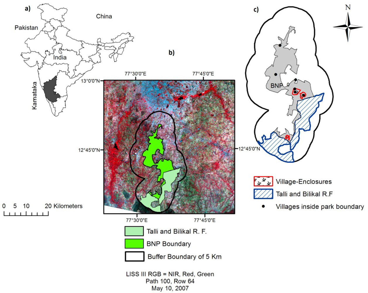
Bannerghatta National Park (BNP) is in the southern part of Karnataka State, 22 km south of the city of Bangalore (Figure 1). BNP is one of the most recent national parks of Karnataka State. It was started in 1971 and declared as a national park in 1974, and it comprises 12 reserve forests [80]. The study area encompasses BNP which is 109 km2 and a buffer of 5 km around the park. Dry deciduous forest and scrub forests are the main vegetation cover inside the BNP with patches of eucalyptus plantation and moist deciduous forest in a few places.
There are seven village communities within BNP, which form three major enclosures inside the park. The fourth enclosure forms a farming estate Ukkada. The buffer area has several hundred village communities, village market areas and small towns. Outside the northern part of the park boundary lays a suburban landscape that is mainly an expansion of Bangalore’s urban area, with a dense road network and residential plots. The western and eastern sections outside the BNP boundary are composed of agricultural village communities. There is a predominance of eucalyptus in the eastern part of the park and coconut palm and mango in the western part of the park. A five km spatial buffer area around BNP acts as the unprotected area of the study. We created a GIS buffer region taking a five km radius extending outside the outer park boundary to compare the land cover change between the buffer and park area which has been a common practice in park effectiveness studies [21]. Moreover we took a five km limit for our GIS buffer because most of the forest cover outside BNP lies within five km of the park boundary range.
2.2. Data Sources
The main data used in the study are four satellite images (Table 1). Landsat MSS 1973 (path 154, row 51), Landsat TM 1992 and 1999 (path 144, row 51), and the 2007 image is IRS LISS III (path 100, row 64). All the image dates are cloud free, dry season images. The BNP boundary is created from topographic maps at 1: 50,000 scales, which were collected from the Survey of India.
2.3. Research Methods
2.3.1 Land-Use and Land-Cover Change Detection Analysis
Land use and land-cover patterns for 1973, 1992, 1999 and 2007 were mapped by using Landsat MSS, TM and IRS LISS III data. The images were corrected for sensor and atmospheric calibration errors using Center for the Study of Institutions, Population, and Environmental Change (CIPEC) methods [81] to minimize the effects caused by using non-anniversary dates with varying sun angle and atmospheric condition [82]. All the data were georectified and resampled to a ground resolution of 30 × 30 m (to match the base information of the Landsat data we thus resampled our finer spatial resolution imagery to this scale) and projected to WGS 84 UTM with a RMSE of less than 0.5 pixels. Nearest neighborhood algorithm was used to resample the images so that the original brightness values of pixels were kept unchanged. The land-cover categories for this study include: (a) native forest (F), (b) tree plantation (P) and c) non-forest (NF) cover. The native forest class includes forest cover with a canopy cover of more than 25%, based on fieldwork (local people’s definition of forest in the region). However, under the Terminalia-Anogeissus Latifolia-Tectona series, this landscape fits in the dry deciduous forest category [83] and thus relatively open scrub areas, dense forest and open forest forms the forest class. This forest class as compared to tree plantation class has a predominance of native species typical for the region and thus will be called ‘native forest’ henceforth. The tree plantation class includes four main species, i.e., Cocos nucifera (palm trees), Eucalyptus cinerea (eucalyptus), Tectona grandis (teak) and Mangifera indica (mango). The non-forest class includes the agricultural land, fallow land, grassland, bare ground, built area and stone waste. The classifications were done using a hybrid approach combining both a supervised (maximum likelihood method) and unsupervised classification using Iterative Self-Organizing Data Analysis Techniques (ISODATA) clustering method. Further, rule based methods were used to refine and separate the tree plantation class from the native forest class using texture layers as the texture of tree plantation class has been found to be very different than that of the native forest class. The overall accuracy of the 2007 classification, assessed on the basis of the training sample points collected during field visits of 2007 and 2008 was 82.14%, with an overall Kappa of 0.7043. Although we acknowledge Kappa’s limited ability as a measure of accuracy, as found by prior study [84], it is a commonly used method in land use land cover analysis [85–87]. Limited field data for validation, and some points from 2008 when change had occurred since the imagery being obtained, limited the overall accuracy to a value of only 82.14%, but imagery was also evaluated by in country experts and field interviews and deemed acceptable for use in this study. If the classification was kept as forest and non-forest much higher accuracy levels were obtained (over 90%). However, the question of tree plantation versus native forest (the two most confused classes) was important to separate as the tree plantations, in terms of their use, are an agricultural crop in this region and so ecologically and socially are a very different type of land cover from native forest. Even though this did act to lower the accuracy of the classifications it was preferred over grouping these two land covers.
2.3.2 Markov Chain Analysis
The Markov chain model is a stochastic model where the model output is based on the probability of transition, Pij, between state i and j. In a landscape with multiple land covers or land uses, the transition probability Pij would be the probability that a land cover type (pixels) i in time t0 changes to land cover type j in time t1. As the transitions are probabilities, it follows that
The transition probabilities are derived from a sample of transitions occurring during some time interval [46]. These probabilities could be shown through the following transition matrix P.
where,
- Vi × Pij = Proportion of land cover of second date,
- Pij = Matrix of probability of land cover transition,
- Vi = Proportion of land cover of first date (Vector),
- i = type of land cover in first date,
- j = type of land cover in second date,
- P11 = the probability that a land cover 1 at first date will change into land cover 1 by second date,
- P12 = the probability that a land cover 1 at first date will change into land cover 2 by second date and so on,
- m = the number of land cover types in the study area.
This transition matrix of Markov chain analysis can be used to predict the future land cover or land use at time t2. The model, however, is not spatially-explicit and does not provide explanation of change processes and overlooks the spatial distribution of land-cover in predicting land-covers [88].
2.3.3. Cellular Automata (CA)
Cellular automata (CA) are spatially dynamic models frequently used for land-use and land-cover change studies. In a CA model, the transition of a cell from one land-cover to another depends on the state of the neighborhood cells [89]. This is based on the idea that a cell will have a higher probability to change to land-cover class ‘A’ than to a land-cover class ‘B’ if the cell is in closer proximity to land-cover class ‘A’. Thus the CA model not only uses the information of the previous state of a land-cover as done by a Markov model but also uses the state of neighborhood cells for its transition rules. CA models have been used widely for land use and land cover (LULC) change analysis especially for forest cover change analysis [89,90]. As such, a CA model can add spatial character to a Markov model and make it a dynamic spatial model.
2.3.4. CA Markov Model
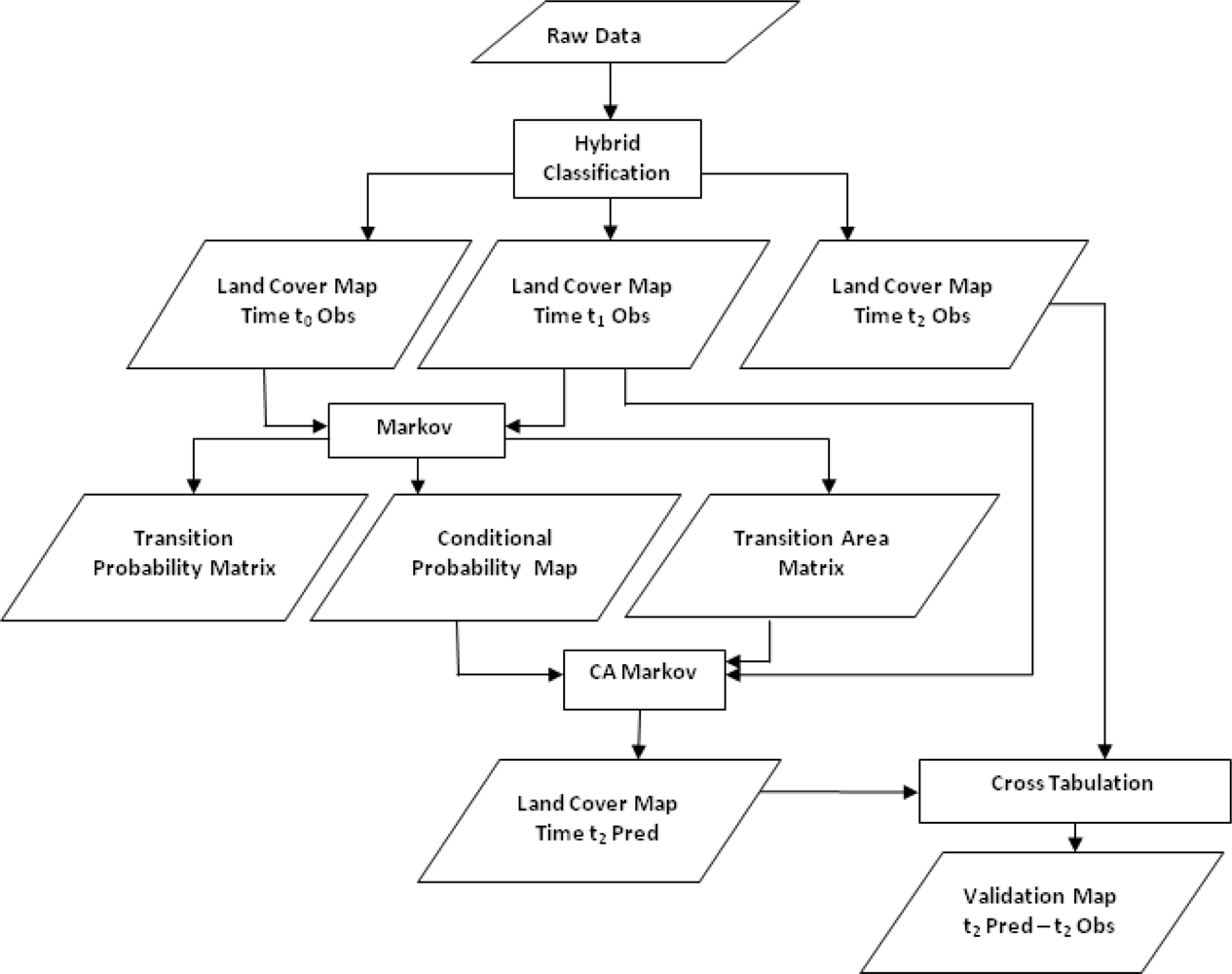
A combined Markov and CA (CA Markov) is used in the present study to predict the land-cover for 1999 and 2007. Four separate models are run. All the models are run in two steps using the Markov and CA Markov module of IDRISI 16. In the first step a Markov model is run using the land-cover maps of 1973–1992, 1992–1999 and 1973–1999 to predict for 1999 and 2007 (Table 2). The outputs of this step are a transition area matrix, a transition probability matrix and a series of transition probability maps (probability of each pixel to a particular land-cover). The transition areas matrix is a text file that records the number of pixels that are expected to change from each land cover type to each other land cover type over the specified number of time units. The transition probability matrix is a text file that records the probability that each land cover category will change to every other category. Transition probability maps are generated for three land-cover classes, i.e., tree plantation, native forest and non-forest. The conditional probability maps report the probability that each land cover type would be found at each pixel after the specified number of time units [78]. As such, these probability maps are calculated as projections for time t2 from the later of the two input land cover images (t1) as shown in Table 2.
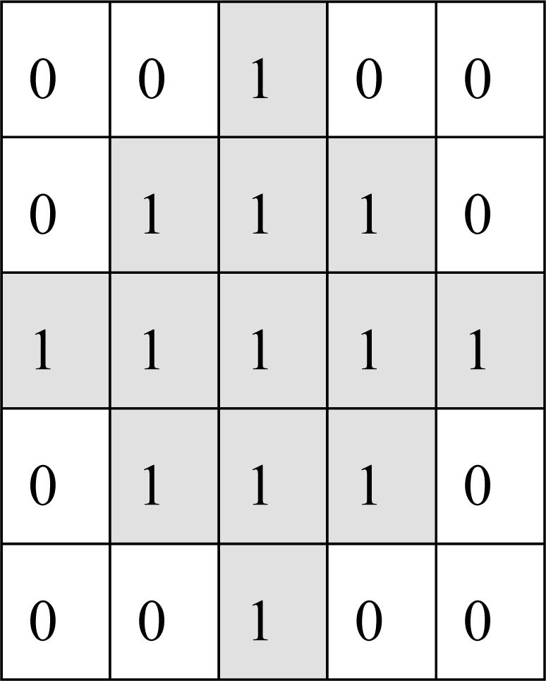
In the second step CA Markov module is used to run the CA analysis using the land cover classification maps of 1992 and 1999 and outputs from the Markov module, i.e., transition area matrix, transition probability maps (Figure 2) and contiguity. The combined cellular automata and Markov chain method of the CA Markov module adds an element of spatial contiguity as well as knowledge of the likely spatial distribution of transitions to Markov chain analysis. In an iterative process the CA Markov module uses the transition probability maps for each land cover to establish the inherent suitability of each pixel for each land cover type but contiguity filter down-weights the suitability of pixels far from existing areas of that class (as of that iteration), thus giving preference to contiguous suitable areas. Contiguity filters of 5 × 5 (Figure 3) were applied to define neighborhoods of each cell [78].
Four different models were run to predict land cover for 2007 and 1999 using 1973, 1992 and 1999 as input maps (Table 2). In doing so, the CA Markov model makes the assumption that the driving factors affecting change in all time periods are same. This assumption is however, not met as the National Forest Policy which banned the felling of trees from national parks was instituted in 1988, which would be applicable in the time period 1992–2007 and 1992–1999 and not in 1973–1992. Although the National Forest Policy was instituted in 1988, here we would consider 1973 to 1992 image dates as pre policy intervention time period assuming that there is a lag effect of implementation of the policy and it would take a number of years to be “seen” in the landscape. Since this study tries to create the land cover in the absence of national level policy intervention, this assumption is important for the present study.
The ‘before–after’ scenario was constructed by comparing the before policy intervention (pre 1992) with the after policy intervention (post 1992) landscape for predicted and observed landscapes. For comparison between observed and predicted landscapes, both individual land covers and land cover trajectories were considered. For change analysis, a post-classification cross tabulation change detection method was used. Moreover, all the comparisons between observed and predicted landscape were divided into three categories of BNP and its surroundings (overall landscape), BNP (inside park) and Buffer (outside park). These comparisons provided us with methods to analyze our objectives of comparing ‘before–after’ and ‘inside–outside’ scenarios.
The next step in model building is validation of a model that is necessary when a predictive model is built, to test how well the model is doing. Validation provides the means to test a model against data that were not used to construct the model [91]. If a model of LULC change is simulated by using time t0 and t1 and then it predicts the change from t1 to t2, in order to evaluate such model performance, the predicted map of time t2 is usually compared with reference map of t2 which is also the observed map of t2 [92]. For our present study, the third (1999obs) and fourth (2007obs) time period should be used as reference maps for validating the corresponding dates predicted maps of 1999pred4 and 2007pred1, 2007pred2 and 2007pred3 since these data were not used to build the respective models [59]. If the predicted 1999pred4 map is similar to reference 1999obs map, we could have said that the model performed well. However, in our case we do not expect good model performance, as this would indicate no policy intervention impact on the landscape. Rather, for this study a weak model prediction of our future dates is expected with an over prediction of forest clearing. If the policy intervention succeeded, then post 1988 we expect a decrease in deforestation and the start of forest recovery. Nevertheless, it is not possible to validate our predicted landscape through direct methods, as the predicted scenarios are hypothetical scenarios representing a landscape that didn’t exist. One indirect way to validate the models would be to compare between the three predicted models of 2007 with observed land cover maps. Within the three models of 2007, we would expect model 2 (Table 3) to perform better in predicting 2007 landscape as it uses a post policy intervention land cover maps (1999) as input and thus would incorporate the present trends of reforestation in our predictive model. Validation was done simply by cross tabulating the predicted and observed land covers of respective years (Figure 2). Using the CA Markov models in this unique manner will therefore allow us to evaluate this policy impact [52].
3. Results
3.1. Land-Use and Land-Cover Projection—Before–After/Inside–Outside
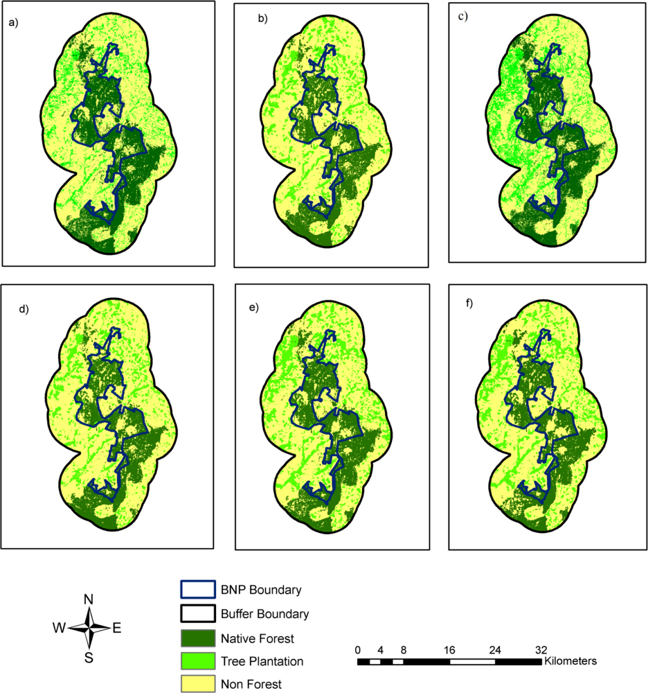
The satellite image analysis of four dates (1973, 1992, 1999, and 2007) show few dominant changes in the actual observed landscape. The overall landscape shows a predominance of non-forest cover for all the dates (58%, 62%, 58%, 51%), which initially increased between 1973 and 1992 but declined post 1992. This decline in non-forest cover in the overall landscape post 1992 could be attributed to the increase in tree plantation outside the park boundary. Inside BNP, native forest cover is the dominant land cover for all the dates. Native forest cover inside BNP declined from 78% to 73% between 1973 and 1992, and then it increased to 74% in 1999 and 77% in 2007. Most of the tree plantation is located outside BNP and it shows an increasing trend (10%, 11%, 15% and 23%). Overall, actual observed landscape shows a trend of declining deforestation and slow recovery of native forest cover inside BNP (a patchy reforestation trend) and a slower decline in native forest cover outside BNP post 1992 (Figures 4 and 5).
A similar inconsistency is noticed between the predicted and observed non forest cover in the overall landscape where non forest cover is 3–8% higher in the predicted landscape than the observed landscape; observed landscape shows a trend of declining non forest cover post 1992 after initial increase between 1973 and 1992 (Figure 5(c)). Inside the park, an opposing trend of predicted and observed non-forest cover could be noticed. The non-forest area is predicted to increase inside the park post 1992 while in reality it declined (Figure 5(f)). It is higher by 5–11% in the predicted landscape than in the observed landscape. Overall, the model fails to predict the observed reforestation trend inside BNP. In the buffer area the models over predict the non-forest area (Figure 5(i)). The disagreement between the predicted and observed landscape is the least in the tree plantation class.
3.2. Change Trajectories Projection
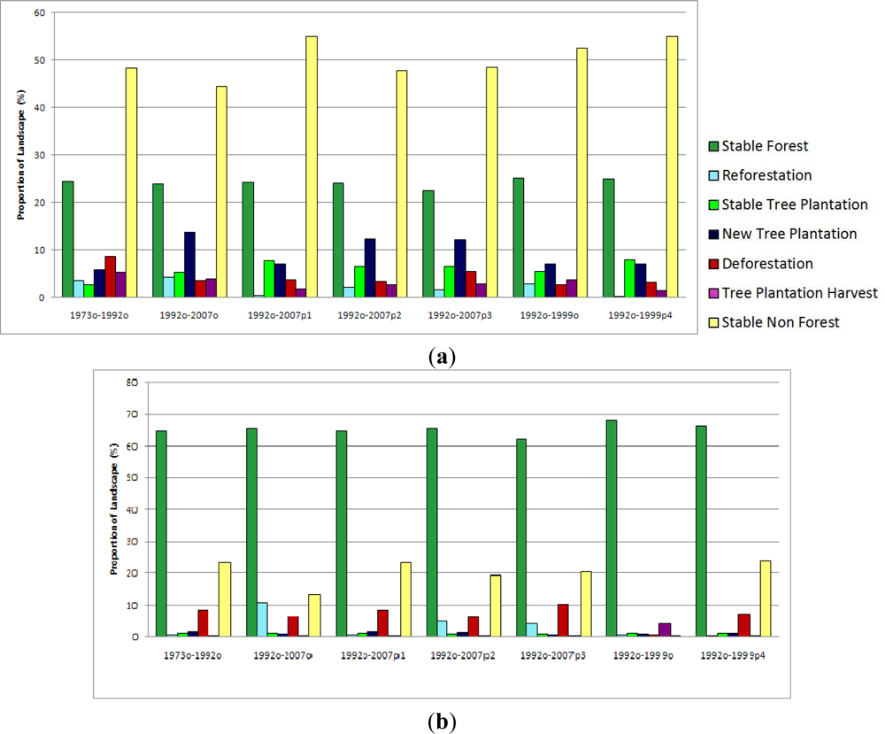
The change trajectories between the observed and predicted land cover classes were compared on a pixel-by-pixel basis to examine the spatial pattern of land cover trajectories (Figures 6 and 7). The two date change trajectory with three land-cover classes gives nine possible land cover trajectories. The land covers that remained unchanged in both the time steps are classed as stable native forest, stable non forest and stable tree plantation. The forest loss would be termed as deforestation in the absence of data availability to give a distinction between deforestation and degradation. Deforestation is defined as any land cover that was native forest in time 1 but changed to non-forest in time 2. Reforestation is categorized as any land cover which was a non forest cover in time 1 but changed to a native forest in time 2. Any land cover that was tree plantation in time 1 and changed to non forest in time 2 is categorized as tree plantation harvest. Land covers, which were non forests in time 1 and changed to tree plantation in time 2, are defined as new tree plantation. The ‘tree plantation to native forest’ and ‘native forest to tree plantation’ trajectories are not shown as they cover <1% of landscape.
The predicted and observed land cover transitions show dissimilarities in three main categories, i.e., deforestation, reforestation and stable non-forest (Figures 6 and 7). The models over predict deforestation by 5–6% post 1992 inside BNP but in the buffer area the predicted deforestation of all the time pairs are in agreement with their respective observed time pairs (Figure 6(b,c)). In the observed landscape, the deforested area actually declined from the first time period (1973–1992) to the second time period inside BNP (post 1992) whereas the predicted landscape shows no decline (Figure 6(b)). A similar trend to deforestation could be observed in the stable non-forest trajectory inside the park, which is over predicted by 8–10% in post 1992 time pairs (Figure 6(b)). The models also over predict the stable non-forest cover in the buffer area post 1992 (Figure 6(c)). Lastly, the models under predicts reforestation inside the park by 5–10% and outside the park by 2–4% in post 1992 time pairs. Inside the park, the actual quantity of reforestation increased from 1973–1992 to 1992–2007 but the models couldn’t predict this increase in reforestation (Figure 6(b,c).
In terms of spatial difference between the observed and predicted land cover transitions, the two-date change trajectory map (Figure 7) shows a higher deforestation inside BNP in the predicted maps as compared to the observed deforestation which has occurred mostly outside either on the edges of the park or near the village enclosures inside the park. The predicted deforestation outside the park is located either in the Talli and the Bilikal Reserve Forest or on the northwestern part outside BNP.
3.3. Model Validation
Figure 8 shows a cross tabulation of observed and predicted land covers of 1999 and 2007. These maps were created to see how well our model performed as compared to our observed landscape. All the models had a general disagreement on the predicted and observed quantity and spatial location of land covers as well as land cover transitions.
However, the results show differences in trend within the models. Model 2 (Table 2) has the best agreement with the observed and predicted of all the models. Model 2 actually uses 1992–1999 (a post policy intervention land cover map) to predict for 2007. The stationarity of driving factor assumption creates a 2007pred2 landscape, which has policy impact. Models that use pre policy intervention land cover maps (model 1 and 4) have weaker predictions, which we expected them to do. Our models (1 and 4) inaccurate predictions are important to us as this validates our idea that the national forest policy of 1988 has a positive effect on the forest cover as observed in our actual landscape but not shown in our models.
4. Discussion
The Cellular Automata Markov (CA Markov) model of land-cover change processes allows us to address questions such as how the land-cover of the BNP and its surrounding would be without any protection or policy intervention, and how the predicted land-cover will differ from the observed land-cover. Although India has followed the exclusionary model of protected area management since the British period, it has also made various revisions, the most recent one came through the National Forest Policy of 1988, which completely banned any harvest of trees from National Parks and protected sanctuaries of India and that included felling of trees for commercial and industrial purposes [31,93]. The CA Markov model was built to evaluate the impact of this national level forest policy change of 1988 in BNP, which was declared as a National Park in 1974.
In the absence of a policy change or protected area status, the forest cover inside BNP and its buffer area would be expected to be equally affected by same socio-economic drivers and proximate causes. With protection and a policy change, the forest cover inside BNP should be better maintained than the forest cover outside BNP. Even though BNP was declared a National Park as early as 1974 and hence given a formal protection, decline in native forest cover and increase in non-forest cover inside the park was observed up until 1992 (Figures 4 and 5). This decline in native forest cover could be driven by various socio-economic activities of village communities both inside and outside the park. Another driving factor could be the felling of trees inside the park for commercial and industrial purposes as in India state forests were managed under ‘working circles’ with a 30-year extraction cycle [93]. Since the socio-economic drivers and proximate causes affecting the park (village communities) are present even today, it could be the National Forest Policy of 1988 and the revisions made (ban on felling of trees) which resulted in the recovery of native forest cover and decline in non forest cover inside the park after 1992. Clearly without the change in the national forest policy of 1988, the trend of decline in native forest cover and increase in non-forest area inside the park since 1973 would have continued until today. The use of the CA Markov model which is commonly criticized for its incapability of incorporating human decision making [74], and thus made the assumption that the driving factors affecting the park would be same in different time steps (pre and post 1992), created a post 1992 landscape of no policy intervention and accordingly predicted a continued decline in native forest cover inside the park even though in reality it increased post 1992. Even if we consider the fact that the quantity and the spatial distribution of native forest and non-forest cover changes in the actual landscape, in the absence of any policy intervention, would not be same as that predicted by our CA Markov model, we can still say that the overall trend of changes would be similar to our predicted landscape. It is possible that in the actual landscape, in the absence of the policy intervention of 1988, a continued commercial and industrial harvest of the forest would result in forest clearing in areas different than shown in our predicted models. Further, the quantity of forest clearing in the actual landscape could have been different than what our models predicted in our actual landscape, in the absence of a policy intervention. Consequently, we should use the quantity and spatial distribution of the forest cover change in our predicted model with caution and use the overall pattern and trend of forest cover change to come to any conclusions.
The policy intervention in this case could be said to have a positive impact in protecting the forest cover of BNP as could be seen from the decline in deforestation and increase in reforestation inside the park in our observed landscape post 1992. Our predicted landscape showed a higher deforestation than what actually occurred inside BNP between 1992–2007 and 1992–1999. The fact that all the models overpredicted deforestation inside the park (Figure 6(b–d,f)) and had a better agreement between the predicted and observed deforestation outside the park in terms of quantity (Figure 6(b,c)) could be an indicator that the driving factors affecting deforestation inside the park may have been different (as assumed here due to the National Forest Policy of 1988). Similarly, our models were bad at predicting reforestation inside the park post 1992 (predicted a lot lower reforestation than actually occurred). In addition, the validation maps (Figure 8) shows that the ‘native forest–non forest’ class (native forest in observed/actual land cover but were predicted to be non forest by the model) were mostly located inside the park and in the Talli and Bilikal Reserve Forest which is under formal protection. Accordingly, we can conclude that the driving factors affecting the park and the buffer were different in the pre and post 1992 landscape as BNP already had a formal protection since 1974. However, this protection was unable to curb the deforestation inside the park. We can say that the Indian government’s policy intervention of 1988 could be the change in the driving factor that resulted in recovery of forest cover inside this park. This could further corroborate the argument that mere creation of national parks will not achieve conservation goals and would only result in more ‘paper parks’ unless accompanied by effective national level policies [94,95] and improved management policies [96]. A similar study of creating a ‘no policy intervention forest cover scenario’ of Pench National Park, India, using a CA Markov model also found discrepancies in the predicted and the observed land cover scenarios and also thus a positive impact of the National forest policy of 1988 on the forest cover [97].
An argument however could be made that there was a decrease in non-forest cover outside BNP post 1992 as well even though there was no formal protection provided to the buffer area and the 1988 revised policy should have no effect on the buffer area. However, this decline in non-forest cover could be because of a reforestation trend outside BNP. Even though there is a reforestation trend in the overall landscape, distinction could be made between the reforestation trend inside and outside the park. Reforestation in the buffer area is tree plantation driven while inside park the forest cover recovery is mostly because of native forest cover increase. This tree plantation driven reforestation could explain the decline in non forest cover outside the park and may be attributed to various social forestry and agro-forestry programs undertaken by state and international agencies to achieve various goals, i.e., fuelwood and fodder for local village communities, wood for industrial and commercial purposes and various ecosystem services [31,97].
Cellular models like CA Markov (probabilistic) models have been criticized for their unreliability in predicting dynamic processes such as LULC affected by human decisions [68] because of their assumptions of stationarity of driving forces in different time steps and so not directly accounting for the driving factors of land cover change [13,59,74]. For this particular study this assumption has been advantageous in validating the presence of different driving factors affecting the forest cover pre and post 1992 [52]. Further, the argument that protection goes to less threatened areas and a PA would maintain forest cover irrespective of any policy intervention [43,98] would be redundant in the present study. This is due to the fact that BNP experienced forest cover decline from 1973 to 1992 and is situated just few miles outside the rapidly growing city of Bangalore, in a densely populated area with seven village communities inside the national park. Such factors are true for many of the PAs of India [99] and make the results of such studies as this, even more relevant. Further a small geographical area with little difference in elevation between the buffer and the park and dense road network makes the national park as accessible and vulnerable to various drivers of deforestation as the buffer would be. Hence, we could say that this shift in India’s forest management policies from a productive forest management to a protected forest management practice with the introduction of the National Forest Policy of 1988 which clearly stated that national parks must contribute to the conservation of soil and environment rather than be exploited for commercial-industrial purposes [31], has had a positive impact on the forest cover of BNP. These results of forest recovery are on a par with the national trend of reforestation and increase in forest cover [5,100,101] and the general consensus in India that PAs are successful in maintaining forest cover [25,52].
While there is an abundance of literature on quantitative assessments of deforestation in and around PAs, more so for dwindling tropical forests [100,102,103], there is a growing literature on tropical reforestation and regrowth [13,14,104–106] which necessitates evaluation of PAs for both deforestation and reforestation trends. Additionally, traditional methods of evaluating PAs have varied (comparison of inside versus outside PA, protected versus non protected forest, past trends versus future trends), but most of these studies still focus on assessing deforestation rates. Nevertheless, evaluation of effectiveness of PAs in tropical forest areas experiencing simultaneous deforestation and reforestation has been successfully done using a CA-Markov modeling approach [12,14,15,52,54]. Our findings of a positive impact of policy intervention on forest cover of BNP and assessment of simultaneous deforestation and reforestation trends using CA Markov methods certainly expands on the literature on present forest transition studies.
CA Markov models are widely used for predicting dynamic spatial phenomenon. The model has been widely used for determination of rangeland dynamics [79], species composition [77], forest succession [107], and a wide range of LULC studies [89,108]. Even though CA models face challenges to incorporate human decision making, they have been nevertheless found them useful for modeling ecological aspects of LULC [13–15,68]. While CA Markov models have been more commonly used to evaluate the impact of protection on a forested landscape by projecting forest cover changes in the future [109,110], we used this model to generate a hypothetical scenario of our present observable landscape without the effect of a policy intervention. We found this modeling approach useful and transferable to other areas where policy evaluation using traditional methods are not possible.
5. Conclusions
This research demonstrates the potential use of satellite remote sensing and Cellular Automata (CA) Markov methods for understanding the effectiveness of policy intervention in conserving forest cover. In this paper we evaluated the Indian National Forest Policy of 1988 and the revisions made to it by building a landscape of no policy intervention using a CA Markov model. A CA Markov model is limited by its capacity to incorporate human decision making and thus assumes a stability of driving factors affecting the park over time. We used this limitation to our advantage in a unique way by creating a modeled landscape that didn’t have the impact of 1988 national forest policy changes. The model generated four different land cover scenarios of Bannerghatta National Park (BNP) and its surroundings for the period 1999 and 2007. Two main methods of comparison: ‘before-after’ and ‘inside-outside’ approaches were taken to evaluate the effectiveness of protected area management and the implications of the national forest policy change on the forest cover of BNP. While most predictive modeling studies aim for their models to do well, we expected weaker model predictions to indicate no impact of the Indian National Forest Policy of 1988 on our landscape. Our findings show a general discrepancy between our predicted and observed landscapes. Deforestation inside the park was predicted to be 5–6% higher than what actually took place in the landscape post 1992. Similarly, predicted reforestation inside park was lower by 5–10% than the actual reforestation in 1999 and 2007 landscapes. The modeled landscape also showed 8–10% higher stable non-forest cover inside BNP than the actual stable non-forest cover. This discrepancy in predicted and observed landscape suggests that had there been no revision in the national level forest policies, BNP would have remained a ‘paper park’ and would have suffered higher levels of deforestation and the recovery of forest cover inside the park would not have been possible.
Although remotely sensed data and the CA Markov model helped to evaluate the effectiveness of Protected Area (PA) management in BNP and its surroundings, the probabilistic nature of the model didn’t allow for in-depth discussion of the various driving factors affecting the deforestation or the reforestation in the region. Spatio-statistical model building, where the land cover changes are fitted with the predictor variables (various socio-economic driving factors and proximate causes) would be imperative in the future to predict forest cover changes in BNP and its surroundings. Such model building would give a much clearer image of the effectiveness of PA management and national level forest policy changes on the land cover change of a region and will help to create more successful management strategies. Although further model building is crucial for understanding the driving factors acting within the landscape, this kind of reverse modeling wherein we are constructing a land cover scenario that is nonexistent (a no policy intervention landscape) is crucial in explaining the impact of a policy intervention. Furthermore, our study implies that the CA Markov modeling approach could be used for evaluating various national level conservation policies by constructing a ‘no policy’ intervention landscape. This novel approach is perfectly suited to such conservation studies and can be used as a preliminary step for more advanced LULCC analysis and model creation.
Acknowledgments
To University of Florida, USA and Ashoka Trust for Research on Ecology and Environment (ATREE), India for providing data and research equipments for the present study. We are also thankful to Dr. Harini Nagendra for providing the LISS III satellite images for 2007 and to the reviewers and editors for their valuable comments and contributions to the manuscript.
References and Notes
- National Research Council (NRC). Trends and Transitions. In Our Common Journey: A Transition toward Sustainability; National Academy Press: Washington, DC, USA, 1999; pp. 59–132. [Google Scholar]
- Geist, H.J.; Lambin, E.F. Proximate causes and underlying driving forces of tropical deforestation. BioScience 2002, 52, 143–150. [Google Scholar]
- Brambilla, M.; Casale, F.; Bergero, V.; Bogliani, G.; Crovetto, G.M.; Falco, R.; Roati, M.; Negri, I. Glorious past, uncertain present, bad future? Assessing effects of land-use changes on habitat suitability for a threatened farmland bird species. Biol. Conserv 2010, 143, 2770–2778. [Google Scholar]
- Angelsen, A.; Kaimowitz, D. Rethinking the causes of deforestation: lessons from economic models. World Bank Res. Obs 1999, 14, 73–98. [Google Scholar]
- Food and Agriculture Organization (FAO). Global Forest Resources Assessment 2010; Food and Agriculture Organization of the United Nations: Rome, Italy, 2010. Available online: http://www.fao.org/forestry/fra/fra2010/en/ (accessed on 12 September 2012).
- Rodrigues, A.S.L.; Andelman, S.J.; Bakarr, M.I.; Boitani, L.; Brooks, T.M.; Cowling, R.M.; Fishpool, L.D.C.; da Fonseca, G.A.B.; Gaston, K.J.; Hoffmann, M.; et al. Effectiveness of the global protected area network in representing species diversity. Nature 2004, 428, 640–643. [Google Scholar]
- Chape, S.; Harrison, J.; Spalding, M.; Lysenko, I. Measuring the extent and effectiveness of protected areas as an indicator for meeting global biodiversity targets. Phil. T. Roy. Soc. B 2005, 360, 443–455. [Google Scholar]
- Loucks, C.; Ricketts, H.T.; Naidoo, R.; Lamoreux, J.; Hoekstra, J. Explaining the global pattern of protected area coverage: Relative importance of vertebrate biodiversity, human activities and agricultural suitability. J. Biogeogr 2008, 35, 1337–1348. [Google Scholar]
- United Nations Environment Programme-World Conservation Monitoring Centre. State of the World’s Protected Areas 2007: An Annual Review of Global Conservation Progress; UNEP-WCMC: Cambridge, UK, 2008. [Google Scholar]
- Jenkins, C.N.; Joppa, L. Expansion of the global terrestrial protected area system. Biol. Conserv 2009, 142, 2166–2174. [Google Scholar]
- Lele, N.; Nagendra, H.; Southworth, J. Accessibility, demography and protection: drivers of forest stability and change at multiple scales in the Cauvery Basin, India. Remote Sens 2010, 2, 306–332. [Google Scholar]
- Tattoni, C.; Ciolli, M.; Ferretti, F.; Cantiani, M.G. Monitoring spatial, temporal pattern of Paneveggio forest (Northern Italy) from 1859 to 2006. iForest 2010, 3, 72–80. [Google Scholar]
- Tattoni, C.; Ciolli, M.; Ferretti, F. The fate of priority areas for conservation in protected areas: A fine-scale Markov chain approach. Environ. Manage 2011, 47, 263–278. [Google Scholar]
- Bracchetti, L. Land-cover changes in a remote area of central Apennines (Italy) and management directions. Landsc. Urban Plan 2012, 104, 157–170. [Google Scholar]
- Cabral, P.; Zamyatin, A. Markov processes in modeling land use and land cover changes in Sintra-Cascais, Portugal. Dyna 2009, 158, 191–198. [Google Scholar]
- Pfaff, A.S.P. What drives deforestation in the Brazilian Amazon?: Evidence from satellite and socioeconomic data. J. Environ. Econ. Manage 1999, 37, 26–43. [Google Scholar]
- Zimmerer, K.S.; Galt, R.E.; Buck, M.V. Globalization and multi-spatial trends in the coverage of protected-area conservation (1980 to 2000). Ambio 2004, 33, 520–529. [Google Scholar]
- Nagendra, H. Do parks work? Impact of protected areas on land cover clearing. Ambio 2008, 37, 330–337. [Google Scholar]
- Brandon, K.; Redford, K.; Sanderson, S. Parks in Peril: People, Politics and Protected Areas; Island Press: Washington, DC, USA, 1998; pp. 1–23. [Google Scholar]
- Bates, D.; Rudel, T.K. The political ecology of conserving tropical rain forests: A cross-national analysis. Soc. Natur. Resour 2000, 12, 619–634. [Google Scholar]
- Nagendra, H.; Southworth, J.; Tucker, C.M.; Karmacharya, M.; Karna, B.; Carlson, L. Monitoring parks through remote sensing: Studies in Nepal and Honduras. Environ. Manage 2004, 33, 1–13. [Google Scholar]
- Agrawal, A.; Ostrom, E. Collective action, property rights, and decentralization in resource use in India and Nepal. Polit. Soc 2001, 29, 485–514. [Google Scholar]
- Briggs, J. The biogeographic and tectonic history of India. J. Biogeogr 2003, 30, 381–388. [Google Scholar]
- Mittermeier, R.A.; Mittermeier, C.G. Megadiversity: Earth’s Biologically Wealthiest Nations, 1st ed; Cemex-Conservation International: Monterrey, Mexico, 2005; pp. 1–501. [Google Scholar]
- Karanth, K.K.; Defries, R. Conservation and management in human-dominated landscapes: Case studies from India. Biol. Conserv 2010, 143, 2865–2869. [Google Scholar]
- Rangarajan, M. India’s Wildlife History; Permanent Black and Ran Thambhore Foundation: New Delhi, India, 2001; pp. 1–135. [Google Scholar]
- Guha, R. Dietrich Brandis and Indian Forestry: A Vision Revisited and Reaffirmed. In Village Voices, Forest Choices: Joint Forest Management in India; Poffenberger, M., McGean, B., Eds.; Oxford University Press: New Delhi, India, 1996; pp. 86–100. [Google Scholar]
- Bandopadhaya, S.; Soumya, S.B.; Shah, P.J. Briefing Paper on Forest Policy: Community Stewardship and Management; Center for Civil Society: New Delhi, India, 2005; pp. 3–6. [Google Scholar]
- Guha, R. Forestry in British and post-British India: A historical analysis in two parts. Econ. Polit. Wkly 1983, 27, 1883. [Google Scholar]
- Saxena, N.C. Policy and Joint Forest Management Series 1: Forest Policy in India; WWF India and International Institute for Environment and Development (IIED): London, UK; p. 1999.
- Arora, D. From state regulation to people’s participation: case of forest management in India. Econ. Polit. Wkly 1994, 29, 691–98. [Google Scholar]
- Karanth, K.K.; Kramer, R.; Qian, S.; Christensen, N.L. Conservation attitudes, perspectives and challenges in India. Biol. Conserv 2008, 141, 2357–2367. [Google Scholar]
- Nagendra, H.; Pareeth, S.; Paul, S.; Dutt, S. Landscapes of protection: Forest change and fragmentation in northern West Bengal, India. Environ. Manage 2009, 44, 853–864. [Google Scholar]
- Balmford, A.; Bennun, L.; Brink, B.T.; Cooper, D.; Côte, I.M.; Crane, P.; Dobson, A.; Dudley, N.; Dutton, I.; Green, R.E.; et al. Ecology: The convention on biological diversity’s 2010 target. Science 2005, 307, 212–213. [Google Scholar]
- Carr, D.L. A tale of two roads: Land tenure, poverty, and politics on the Guatemalan frontier. Geoforum 2006, 37, 94–103. [Google Scholar]
- Oliveira, P.J.C.; Asner, G.P.; Knapp, D.E.; Almeyda, A.; Galvan-Gildemeister, R.; Keene, S.; Raybin, R.F.; Smith, R.C. Land-use allocation protects the peruvian amazon. Science 2007, 317, 1233–1236. [Google Scholar]
- Andam, K.S.; Ferraro, P.J.; Pfaff, A.; Sanchez-Azofeifa, G.A.; Robalino, J.A. Measuring the effectiveness of protected area networks in reducing deforestation. PNAS 2008, 105, 16089–16094. [Google Scholar]
- Pffaf, A.; Robalino, J.A.; Sanchez-Azofeifa, G.A.; Andam, K.S.; Ferraro, P.J. Park location affects forest protection: land characteristics cause differences in park impacts across Costa Rica. B.E. J. Econom. Anal. Policy 2009, 9, 1–24. [Google Scholar]
- Bruner, A.G.; Gullison, R.E.; Rice, R.E.; da Fonseca, G.A.B. Effectiveness of parks in protecting tropical biodiversity. Science 2001, 291, 125–128. [Google Scholar]
- Sanchez-Azofeifa, G.A.; Daily, G.C.; Pfaff, A.S.P.; Busch, C. Integrity and isolation of Costa Rica’s national parks and biological reserves: Examining the dynamics of land-cover change. Biol. Conserv 2003, 109, 123–135. [Google Scholar]
- Naughton-Treves, L.; Holland, M.B.; Brandon, K. The role of protected areas in conserving biodiversity and sustaining local livelihoods. Annu. Rev. Environ. Resour 2005, 30, 219–252. [Google Scholar]
- Nepstad, D.; Schwartzman, S.; Bamberger, B.; Santilli, M.; D, R.A.Y.; Schlesinger, P.; Lefebvre, P.; Alencar, A.; Prinz, E.; Fiske, G.; Rolla, A. Inhibition of Amazon deforestation and fire by parks and indigenous lands. Conserv. Biol 2006, 20, 65–73. [Google Scholar]
- Joppa, L.N.; Loarie, S.R.; Pimm, S.L. On the protection of “protected areas”. PNAS 2008, 105, 6673–6678. [Google Scholar]
- Joppa, L.; Pfaff, A. Reassessing the forest impacts of protection. Ann. N.Y. Acad. Sci 2010, 1185, 135–149. [Google Scholar]
- Gadgil, M.; Prasad, S.N.; Ali, R. Forest management and forest policy in India: A critical review. Soc. Action (N.Y.) 1983, 33, 127–155. [Google Scholar]
- Hartter, J.; Southworth, J. Dwindling resources and fragmentation of landscapes around parks: Wetlands and forest patches around Kibale National Park, Uganda. Landsc. Ecol 2009, 24, 643–656. [Google Scholar]
- Hudak, A.T.; Wessman, C.A. Textural analysis of historical aerial photography to characterise woody plant encroachment in South African savanna. Remote Sens. Environ 1998, 66, 317–330. [Google Scholar]
- Lambin, E.F. Modelling and monitoring land-cover change processes in tropical regions. Prog. Phys. Geog 1997, 21, 375–393. [Google Scholar]
- Mertens, B.; Lambin, E.F. Land cover change trajectories in Southern Cameroon. Ann. Assoc. Am. Geogr 2000, 90, 467–494. [Google Scholar]
- Southworth, J.; Nagendra, H.; Munroe, D.K. Are parks working? Exploring human–environment tradeoffs in protected area conservation. Appl. Geogr 2006, 26, 87–95. [Google Scholar]
- Cheong, So-Min.; Brown, D.; Kok, K.; López-Carr, D. Mixed Methods in Land Change Research: Towards Integration. Trans.Inst. Br. Geogr 2012, 37, 8–12. [Google Scholar]
- Mondal, P.; Southworth, J. Evaluation of conservation interventions using a cellular Automata-Markov model. For. Ecol. Manage 2010, 260, 1716–1725. [Google Scholar]
- Liu, M.; Hu, Y.; Chang, Y.; He, X.; Zhang, W. Land use and land cover change analysis and prediction in the upper reaches of the Minjiang River, China. Environ. Manage 2009, 43, 899–907. [Google Scholar]
- Houet, T.; Hubert-Moy, L. Modelling and projecting land-use and land-cover changes with a cellular automaton in considering landscape trajectories: an improvement for simulation of plausible future states. EARSeL eProc 2006, 5, 6–76. [Google Scholar]
- Weinstein, D.; Shugart, H. Ecological Modeling of Landscape Dynamics. In Disturbance and Ecosystems; Mooney, H.A., Gordon, M., Eds.; Springer-Verlag: New York, NY, USA, 1983; pp. 29–45. [Google Scholar]
- Baker, L.W. A review of models of landscape change. Landsc. Ecol 1989, 2, 111–133. [Google Scholar]
- Sklar, F.H.; Costanza, R. The Development of Dynamic Spatial Models for Landscape Ecology: A Review. In Quantitative Methods in Landscape Ecology; Turner, M.G., Gardner, R.H., Eds.; Springer-Verlag: New York, NY, USA, 1991; pp. 239–288. [Google Scholar]
- Brown, D.G.; Walker, R.; Manson, S.; Seto, K.C. Modeling Land Use and Land Cover Change. In Land Change Science: Observing, Monitoring, and Understanding Trajectories of Change on the Earth’s Surface; Gutman, G., Janetos, A., Justice, C., Moran, E., Mustard, J., Rindfuss, R., Skole, D., Turner, B.L., II., Cochrane, M.A., Eds.; Kluwer Academic Publishers: Dordrecht, The Netherlands, 2004; pp. 395–409. [Google Scholar]
- Pontius, R.G.J.; Malanson, J. Comparsion of the structure and accuracy of two land change models. Int. J. Geogr. Inf. Sci 2005, 19, 243–265. [Google Scholar]
- Mertens, B.; Lambin, E.F. Spatial modeling of deforestation in southern Cameroon: Spatial disaggregation of diverse deforestation processes. Appl. Geogr 1997, 17, 143–162. [Google Scholar]
- Hastie, T.; Tibshirani, R. Generalized additive models. Stat. Sci 1986, 1, 297–318. [Google Scholar]
- Brown, D.G.; Goovaerts, P.; Burnicki, A.; Li, M.Y. Stochastic simulation of land-cover change using geostatistics and generalized additive models. Photogramm. Eng. Remote Sensing 2002, 68, 1051–1061. [Google Scholar]
- Tewolde, M.G.; Cabral, P. Urban sprawl analysis and modeling in Asmara, Eritrea. Remote Sens 2011, 3, 2148–2165. [Google Scholar]
- Fitz, H.C.; DeBellevue, E.B.; Costanza, R.; Boumans, R.; Maxwell, T.; Wainger, L.; Sklar, F.H. Development of a general ecosystem model for a range of scales and ecosystems. Ecol. Model 1996, 88, 263–295. [Google Scholar]
- Wu, Y.; Sklar, F.H.; Gopu, K.; Rutchey, K. Fire simulations in the Everglades landscape using parallel programming. Ecol. Model 1996, 93, 113–124. [Google Scholar]
- Voinov, A.; Costanza, R.; Wainger, L.; Boumans, R.; Villa, F.; Maxwell, T.; Voinov, H. Patuxent landscape model: Integrated ecological economic modeling of a watershed. Environ. Modell. Softw 1999, 14, 473–491. [Google Scholar]
- Clarke, K.C.; Gaydos, L.J. Loose-coupling a cellular automation model and GIS: Long-term urban growth prediction for San Francisco and Washington/Baltimore. Int. J. Geogr. Inf. Sci 1998, 12, 699–714. [Google Scholar]
- Parker, C.D.; Manson, M.S.; Janssen, A.M.; Hoffmann, J.M.; Deadman, P. Multi-Agent Systems for the simulation of land-use and land-cover change: A review. Ann. Assoc. Am. Geogr 2003, 93, 314–337. [Google Scholar]
- Manson, S.M. Agent-Based Dynamic Spatial Simulation of Land-Use/Cover Change in the Yucatán Peninsula, Mexico. Proceedings of the Fourth International Conference on Integrating GIS and Environmental Modeling (GIS/EM4), Banff, Canada, 2– 8 September 2000.
- Urban, D.L.; Wallin, D.O. Introduction to Markov Models. In Learning Landscape Ecology: A Practical Guide to Concepts and Techniques; Gergel, S.E., Turner, M.G., Eds.; Springer-Verlag: New York, NY, USA, 2002; pp. 35–48. [Google Scholar]
- Muller, R.M.; Middleton, J. A Markov model of land-use change dynamics in the Niagara region, Ontario, Canada. Landsc. Ecol 1994, 9, 151–157. [Google Scholar]
- Qihao, W. Land use change analysis in the Zhujiang Delta of China using satellite remote sensing, GIS and stochastic modeling. J. Environ. Manage 2002, 64, 273–284. [Google Scholar]
- Usher, M.B. Statistical Models of Succession. In Plant Succession: Theory and Prediction; Gelnn-Lewin, D.C., Peet, R.K., Veblen, T.T., Eds.; Chapman and Hall: London, UK, 1992; pp. 215–248. [Google Scholar]
- Briassoulis, H. Analysis of Land Use Change: Theoretical and Modelling Approaches. In The Web Book of Regional Science; Loveridge, S., Ed.; Regional Research Institute, West Virginia University: Morgantown, WV, USA, 2000. [Google Scholar]
- Barringer, T.H.; Robinson, V.B. Stochastic Models of Cover Class Dynamics. Proceedings of the 15th International Symposium on Remote Sensing of the Environment, Ann Arbor, MI, USA, 1 January 1981; pp. 125–144.
- Alig, R.J. Modeling Acreage Changes in Forest Ownerships and Cover Types in the Southeast, 3rd ed; US Department of Argriculture, Forest Service, Rocky Mountain Forest and Range Experiment Station: Fort Collins, CO, USA, 1985; pp. 1–14. [Google Scholar]
- Silvertown, J.; Holtier, S.; Johnson, J.; Dale, P. Cellular Automaton models of interspecific competition for space-the effect of pattern on process. J. Ecol. 1992, 80, 527–533. [Google Scholar]
- Clark Labs. IDRISI Geographic Information Systems and Remote Sensing Software; Clark Labs: Worcester, MA, USA, 2006. [Google Scholar]
- Li, H.; Reynolds, J.F. Modeling Effects of Spatial Pattern, Drought, and Grazing on Rates of Rangel and Degradation: A Combined Markov and Cellular Automaton Approach. In Scale in Remote Sensing and GIS; Quattrochi, D.A., Goodchild, M.F., Eds.; Lewis Publishers: Boca Raton, FL, USA, 1997; pp. 211–230. [Google Scholar]
- Radha Devi, A. Karnataka Forest Department Master Plan for Consolidation of Bannerghatta National Park Boundaries and Elephant Corridors; Government of Karnataka: Kalkere, Bangalore, 2003; p. 2. [Google Scholar]
- Green, G.M.; Schweik, C.M.; Randolf, J.C. Retrieving Land-Cover Change Information from Landsat Satellite Images by Minimizing Other Sources of Reflectance Variability. In Seeing the Forest and the Trees: Human-Environment Interactions in Forest Ecosystems; Moran, E.F., Ostrom, E., Eds.; MIT Press: Cambridge, MA, USA, 2005; pp. 131–160. [Google Scholar]
- Jensen, J.R. Introductory Digital Image Processing: A Remote Sensing Perspective; Pearson Prentice Hall: Upper Saddle River, NJ, USA, 2005. [Google Scholar]
- Champion, H.G.; Seth, S.K. A Revised Survey of Forest Types of India; Government of India: New Delhi, India, 1968. [Google Scholar]
- Pontius, R.G. Quantification error versus location error in comparison of categorical maps. Photogramm. Eng. Remote Sensing 2000, 66, 1011–1016. [Google Scholar]
- Foody, G.M. Status of land cover classification accuracy assessment. Remote Sens. Environ 2002, 80, 185–201. [Google Scholar]
- Petit, C.; Scudder, T.; Lambin, E. Quantifying processes of land-cover change by remote sensing: resettlement and rapid land-cover changes in south-eastern Zambia. Int. J. Remote Sens 2001, 22, 3435–3456. [Google Scholar]
- Southworth, J.; Munroe, D.K.; Nagendra, H. Land cover change and landscape fragmentation: Comparing the utility of continuous and discrete analyses for a western Honduras region. Agric. Ecosyst. Environ 2004, 101, 185–205. [Google Scholar]
- Lambin, E.F. Modeling Deforestation Processes: A Review; European Commission: Luxemburg, 1994; pp. 1–113. [Google Scholar]
- Verburg, P.H.; de Nijs, T.C.M.; Ritsema van Eck, J.; Visser, H.; de Jong, K.; A. Method to analyse neighbourhood characteristics of land use patterns. Comput. Environ. Urban Syst 2004, 28, 667–690. [Google Scholar]
- Messina, J.P.; Walsh, S.J. 2.5D Morphogenesis: Modeling landuse and landcover dynamics in the Ecuadorian Amazon. Plant Ecol 2001, 156, 75–88. [Google Scholar]
- Haefner, J.W. Modeling Biological Systems: Principles and Applications; Chapman and Hall: New York, NY, USA, 1996; pp. 144–177. [Google Scholar]
- Pontius, R.G.; Huffaker, D.; Denman, K. Useful techniques of validation for spatially explicit land-change models. Ecol. Model 2004, 179, 445–461. [Google Scholar]
- Ministry of Environment and Forests (MOEF). National Forest Policy 1988; Government of India: New Delhi, India, 1988. [Google Scholar]
- McNeely, J.A. Expanding Partnerships in Conservation; Island Press: Washington DC, USA, 1995; pp. 1–302. [Google Scholar]
- Chape, S.; Harrison, J.; Spalding, M.; Lysenko, I. Measuring the extent and effectiveness of protected areas as an indicator for meeting global biodiversity targets. Phil. T. Roy. Soc. B 2005, 360, 443–455. [Google Scholar]
- Hocking, M.; Stolton, S.; Dudley, N. Evaluating Effectiveness: A Framework for Assessing Management of Protected Areas; IUCN: Gland, Switzerland, and Cambridge, UK, 2000; pp. 1–105. [Google Scholar]
- Nagendra, H. Drivers of regrowth in South Asia’s human impacted forests. Curr. Sci 2009, 97, 1586–1592. [Google Scholar]
- Pressey, R.L.; Whish, G.L.; Barrett, T.W.; Watts, M.E. Effectiveness of protected areas in north-eastern New South Wales: recent trends in six measures. Biol. Conserv 2002, 106, 57–69. [Google Scholar]
- Nagendra, H.; Pareeth, S.; Ghate, R. People within parks—forest villages, land-cover change and landscape fragmentation in the Tadoba Andhari Tiger Reserve, India. Appl. Geogr 2006, 26, 96–112. [Google Scholar]
- Rudel, T.K.; Coomes, O.T.; Moran, E.; Achard, F.; Angelsen, A.; Xu, J.; Lambin, E. Forest transitions: Towards a global understanding of land use change. Global Environ. Change A 2005, 15, 23–31. [Google Scholar]
- Grainger, A. The Bigger Picture-Tropical Forest Change in Context, Concept and Practice. In Reforesting Landscapes: Linking Pattern and Process, Landscape Series 10; Nagendra, H., Southworth, J., Eds.; Springer: Dordrecht, The Netherlands, 2009; pp. 15–44. [Google Scholar]
- DeFries, R.S.; Hansen, A.; Newton, A.C.; Hansen, M.C. Increasing isolation of protected areas in tropical forests over the past twenty years. Ecol. Appl 2005, 15, 19–26. [Google Scholar]
- Southworth, J.; Nagendra, H. Reforestation: Challenges and Themes in Reforestation Research. In Reforesting Landscapes: Linking Pattern and Process, Landscape Series 10; Nagendra, H., Southworth, J., Eds.; Springer: Dordrecht, The Netherlands, 2009; pp. 1–14. [Google Scholar]
- Munroe, D.K.; Southworth, J.; Tucker, C.M. Modeling spatially and temporally complex land cover change: The case of Western Honduras. Prof. Geogr 2004, 56, 544–559. [Google Scholar]
- Nagendra, H.; Pareeth, S.; Sharma, B.; Schweik, C.M.; Adhikari, K.R. Forest fragmentation and regrowth in an institutional mosaic of community, government and private ownership in Nepal. Landsc. Ecol 2008, 23, 41–54. [Google Scholar]
- Sitzia, T.; Semenzato, P.; Trentanovi, G. Natural reforestation is changing spatial patterns of rural mountain and hill landscapes: A global overview. For. Ecol. Manage 2010, 259, 1354–1362. [Google Scholar]
- Alonso, D.; Sole, R.V. The DivGame simulator: A stochastic cellular automata model of rainforest dynamics. Ecol. Model 2000, 133, 131–141. [Google Scholar]
- Srinivasan, S. Linking land use and transportation in a rapidly urbanizing context: A study in Delhi, India. Transportation 2005, 32, 87–104. [Google Scholar]
- García-Frapolli, E.; Ayala-Orozco, B.; Bonilla-Moheno, M.; Espadas-Manrique, C.; Ramos-Fernandez, G. Biodiversity conservation, traditional agriculture and ecotourism: Land cover/land use change projections for a natural protected area in the northeastern Yucatan Peninsula, Mexico. Landsc. Urban Plan 2007, 83, 137–153. [Google Scholar]
- Peterson, L.K.; Bergen, K.M.; Brown, D.G.; Vashchuk, L.; Blam, Y. Forested land-cover patterns and trends over changing forest management eras in the Siberian Baikal region. For. Ecol. Manage 2009, 257, 911–922. [Google Scholar]
Figure 1.
Map showing the study area of BNP and 5 km buffer around the park boundary. (a) Location of the study area in India. (b) Location of BNP in satellite image from LISS III. (c) BNP and a buffer of 5 km showing the villages inside the park and Talli reserve forest (R. F) in the south-eastern part and Bilikal R.F. on the southern part of the park.

Figure 2.
Method of land cover classification and CA Markov model. Steps leading to the prediction of land-cover classes.
Figure 2.
Method of land cover classification and CA Markov model. Steps leading to the prediction of land-cover classes.

Figure 3.
5 × 5 mean contiguity filter applied in CA Markov module.

Figure 4.
Land covers for the study area with Park boundary and a buffer of 5 km from the park boundary. (a) 1999obs (b) 1999pred4 (c) 2007obs (d) 2007pred1 (e) 2007pred2 (f) 2007pred3 (See Table 4 for area). Observed land-covers for a given year is denoted by ‘obs’ and predicted land-covers for a given year is denoted by ‘pred’.

Figure 5.
Observed and predicted land covers of from 1973 to 2007 for the overall landscape (total area = 629.82 km2), BNP (total area = 105.48 km2), and the buffer area (total area = 524.34 km2), showing changes in Native forest: (a–c), Tree Plantation: (d–f) and Non-Forest: (g–i). O = Observed land cover, P = Predicted land cover.


Figure 6.
Two-date change trajectories observed vs. predicted land cover transition for (a) BNP and its surroundings, (b) BNP and (c) Buffer Map showing the study area with Park boundary and a buffer of 5 km from the park boundary.
Figure 6.
Two-date change trajectories observed vs. predicted land cover transition for (a) BNP and its surroundings, (b) BNP and (c) Buffer Map showing the study area with Park boundary and a buffer of 5 km from the park boundary.


Figure 7.
Two-date change trajectory maps giving a comparison of observed vs. predicted land cover transitions for (a) 1992obs–2007obs, (b) 1992obs–2007pred1, (c) 1992obs–2007pred2, (d) 1992obs–2007pred3, (e) 1992obs–1999obs, and (f) 1992obs–1999pred4.
Figure 7.
Two-date change trajectory maps giving a comparison of observed vs. predicted land cover transitions for (a) 1992obs–2007obs, (b) 1992obs–2007pred1, (c) 1992obs–2007pred2, (d) 1992obs–2007pred3, (e) 1992obs–1999obs, and (f) 1992obs–1999pred4.

Figure 8.
Validation maps of observed land cover vs. predicted land cover for dates (a) 2007obs–2007pred1, (b) 2007obs–2007pred2, (c) 2007obs–2007pred3 and (d) 1999obs–1999pred4. Observed land-covers for a given year is denoted by ‘obs’ and predicted land-covers for a given year is denoted by ‘pred’.


| Sensors | Month/Day | Year | Spatial Resolution (m) | Path/Row |
|---|---|---|---|---|
| Landsat MSS | 02/27 | 1973 | 60 | 154/51 |
| Landsat TM | 01/14 | 1992 | 28.5 | 144/51 |
| Landsat TM | 02/02 | 1999 | 30 | 144/51 |
| IRS LISS III | 05/10 | 2007 | 23.5 | 100/64 |
Table 2.
Four Cellular automata (CA) Markov models predicting 1999 and 2007 land-covers. Observed land-covers for a given year is denoted by ‘obs’ and predicted land-covers for a given year is denoted by ‘pred’.
| Step 1 of Markov Chain Analysis
| ||||
|---|---|---|---|---|
| Time T0 | Time T1 | Land Cover Characteristics | Time T2 | |
| Model 1 | 1973obs | 1992obs | No Policy Intervention | 2007pred1 |
| Model 2 | 1992obs | 1999obs | Policy Intervention | 2007pred2 |
| Model 3 | 1973obs | 1999obs | Combined policy Intervention and non policy intervention | 2007pred3 |
| Model 4 | 1973obs | 1992obs | No Policy Intervention | 1999pred4 |
Table 3.
Probability of change for four models based on Markov chain analysis. F = Native Forest, P = Tree Plantation and NF = Non-Forest.
| Probability of Change to Land Cover: | ||||||||||||
|---|---|---|---|---|---|---|---|---|---|---|---|---|
| Change from Given | Model 1 | Model 2 | Model 3 | Model 4 | ||||||||
| Land Cover: | F | P | NF | F | P | NF | F | P | NF | F | P | NF |
| F | 0.650 | 0.027 | 0.321 | 0.741 | 0.037 | 0.220 | 0.749 | 0.000 | 0.250 | 0.716 | 0.013 | 0.269 |
| P | 0.024 | 0.321 | 0.654 | 0.038 | 0.425 | 0.534 | 0.002 | 0.462 | 0.535 | 0.007 | 0.392 | 0.600 |
| NF | 0.097 | 0.178 | 0.724 | 0.084 | 0.223 | 0.692 | 0.0541 | 0.220 | 0.725 | 0.076 | 0.176 | 0.747 |
Table 4.
Observed and predicted land-covers of 2007 and 1999 in BNP and it surroundings. (a) Observed and predicted land-covers BNP and its Surroundings (Buffer). (b) Observed and predicted land-covers BNP (c) Observed and predicted land-covers of the Buffer area.
| Land-cover | Observed-99 | Observed-07 | Model 1 Predicted-07 | Model 2 Predicted-07 | Model 3 Predicted-07 | Model 4 Predicted-99 | ||||||
|---|---|---|---|---|---|---|---|---|---|---|---|---|
| (a) | Area (km2) | Total Area (%) | Area (km2) | Total Area (%) | Area (km2) | Total Area (%) | Area (km2) | Total Area (%) | Area (km2) | Total Area (%) | Area (km2) | Total Area (%) |
| Native Forest | 177.15 | 28.13 | 178.19 | 28.29 | 155.56 | 24.70 | 165.79 | 26.32 | 153.04 | 24.30 | 157.75 | 25.05 |
| Tree Plantation | 81.9 | 13.00 | 124.22 | 19.72 | 93.84 | 14.90 | 124.36 | 19.75 | 119.78 | 19.02 | 95.20 | 15.12 |
| Non Forest | 370.76 | 58.86 | 327.40 | 51.98 | 380.42 | 60.40 | 339.67 | 53.93 | 356.99 | 56.68 | 376.86 | 59.84 |
| (b) | ||||||||||||
| Native Forest | 78.03 | 73.98 | 81.10 | 76.90 | 68.95 | 65.37 | 74.49 | 70.63 | 70.60 | 66.94 | 70.09 | 66.45 |
| Tree Plantation | 2.61 | 2.47 | 3.58 | 3.39 | 3.19 | 3.03 | 4.39 | 4.16 | 2.31 | 2.19 | 2.45 | 2.33 |
| Non Forest | 24.82 | 23.82 | 20.79 | 19.71 | 33.33 | 31.60 | 26.59 | 25.21 | 32.56 | 30.87 | 32.93 | 31.23 |
| (c) | ||||||||||||
| Native Forest | 99.12 | 18.90 | 97.09 | 18.52 | 86.61 | 16.52 | 91.30 | 17.41 | 82.44 | 15.72 | 87.67 | 16.72 |
| Tree Plantation | 79.28 | 15.12 | 120.64 | 23.01 | 90.65 | 17.29 | 119.97 | 22.88 | 117.47 | 22.40 | 92.75 | 17.69 |
| Non Forest | 345.93 | 65.97 | 306.61 | 58.48 | 347.09 | 66.19 | 313.07 | 59.71 | 324.43 | 61.87 | 343.93 | 65.59 |
Share and Cite
MDPI and ACS Style
Adhikari, S.; Southworth, J. Simulating Forest Cover Changes of Bannerghatta National Park Based on a CA-Markov Model: A Remote Sensing Approach. Remote Sens. 2012, 4, 3215-3243. https://0-doi-org.brum.beds.ac.uk/10.3390/rs4103215
AMA Style
Adhikari S, Southworth J. Simulating Forest Cover Changes of Bannerghatta National Park Based on a CA-Markov Model: A Remote Sensing Approach. Remote Sensing. 2012; 4(10):3215-3243. https://0-doi-org.brum.beds.ac.uk/10.3390/rs4103215
Chicago/Turabian StyleAdhikari, Sanchayeeta, and Jane Southworth. 2012. "Simulating Forest Cover Changes of Bannerghatta National Park Based on a CA-Markov Model: A Remote Sensing Approach" Remote Sensing 4, no. 10: 3215-3243. https://0-doi-org.brum.beds.ac.uk/10.3390/rs4103215