Structural Uncertainty in Model-Simulated Trends of Global Gross Primary Production

 ,
,
Abstract
: Projected changes in the frequency and severity of droughts as a result of increase in greenhouse gases have a significant impact on the role of vegetation in regulating the global carbon cycle. Drought effect on vegetation Gross Primary Production (GPP) is usually modeled as a function of Vapor Pressure Deficit (VPD) and/or soil moisture. Climate projections suggest a strong likelihood of increasing trend in VPD, while regional changes in precipitation are less certain. This difference in projections between VPD and precipitation can cause considerable discrepancies in the predictions of vegetation behavior depending on how ecosystem models represent the drought effect. In this study, we scrutinized the model responses to drought using the 30-year record of Global Inventory Modeling and Mapping Studies (GIMMS) 3g Normalized Difference Vegetation Index (NDVI) dataset. A diagnostic ecosystem model, Terrestrial Observation and Prediction System (TOPS), was used to estimate global GPP from 1982 to 2009 under nine different experimental simulations. The control run of global GPP increased until 2000, but stayed constant after 2000. Among the simulations with single climate constraint (temperature, VPD, rainfall and solar radiation), only the VPD-driven simulation showed a decrease in 2000s, while the other scenarios simulated an increase in GPP. The diverging responses in 2000s can be attributed to the difference in the representation of the impact of water stress on vegetation in models, i.e., using VPD and/or precipitation. Spatial map of trend in simulated GPP using GIMMS 3g data is consistent with the GPP driven by soil moisture than the GPP driven by VPD, confirming the need for a soil moisture constraint in modeling global GPP.1. Introduction
Estimation of global vegetation Gross Primary Production (GPP) and Net Primary Production (NPP) and their interannual variations are critical for understanding the feedbacks between the biosphere and the atmosphere. Ecosystem carbon models, inversion models, and inventories have been used for assessing global land primary production, generating total annual global estimates of GPP and NPP converging around 120 [1] and 60 [2] Pg·C·yr−1, respectively. Meanwhile, Net Biome Productivity (NBP), the net carbon accumulation by ecosystems [3], was estimated just 2% of GPP for the 1990s [4]. Therefore, estimation of interannual variations of GPP and NPP are also important as well as their total magnitudes for understanding NBP response to CO2 emissions and changes in climate. To elucidate the mechanisms that cause the interannual variation in GPP, we need to rely on bottom up modeling approaches [5]. However, in contrast to total magnitude of GPP, there is no consensus on interannual variation in global GPP or NPP even for the last few decades with satellite observations (for example, [6,7]).
One reason for the models failing to reach agreement on the interannual variations of GPP is the oversimplification of the simulated responses of vegetation to climate variability. By tuning the model parameters to match their output to the data from validation sites, even simple models can provide a reasonable estimate of total GPP [8,9]. Indeed, as more validation data are becoming available, the annual magnitudes of global GPP and NPP estimations from different models have been converging [1,2]. However, it is another issue whether those simple models tuned to acceptable annual GPP range can produce realistic interannual variations in estimated carbon fluxes. In addition, not enough long-term data are available to validate the model results globally on inter-annual time scales.
The recent availability of a 30-year satellite record of Global Inventory Modeling and Mapping Studies (GIMMS) 3g data, focus of this special issue, from NOAA/AVHRR provides an unprecedented opportunity to examine the interpretation of long-term GPP simulations by simple models. In this study, we focus on the effect of drought stress on the interannual variation in GPP, and assess the structural uncertainty in model-simulated trends of global GPP. Reductions in GPP caused by drought stress can be modeled through increases in Vapor Pressure Deficit (VPD) and/or reductions in precipitation via soil moisture. Because time series of VPD and precipitation are generally highly correlated, some models use only VPD sub-models or only soil moisture sub-models to simulate the impact of drought stress on GPP [10]. Short-term comparisons have shown that VPD-only models can produce variations in GPP that are similar to the ones obtained from models with both VPD and soil moisture sub-models [11]. These similarities are not surprising when precipitation and VPD trends are coherent, but this is not necessarily always the case. For example, it has been reported that while global warming-induced increases in VPD were observed [6], global total precipitation did not show a significant trend for the last three decades [12,13]. In this case, we would expect the VPD-only models to produce incorrect time series of GPP estimates. Furthermore, according to the Coupled Model Intercomparison Project Phase 5 (CMIP5), reduction in relative humidity with global warming was expected to continue over the 21st century [14], while globally averaged precipitation was projected to increase with high uncertainty around regional estimates [15]. Therefore, it is crucial to clarify how model structure of drought stress affects the interannual variations in GPP. To address this question, we used the Terrestrial Observation and Prediction System model (TOPS) [16] to produce global GPP estimates from 1982 to 2009 using GIMMS 3g data, and analyze how VPD and soil moisture influence the interannual variation in global GPP.
2. Data and Methods
2.1. The Terrestrial Observation and Prediction System Model (TOPS)
TOPS is a diagnostic ecosystem process model that simulates the fluxes of energy, carbon, and water through vegetation in response to climate and weather variability [16]. TOPS employs a Light Use Efficiency (LUE) model to calculate GPP [17], as follows:
Soil moisture is simulated using a one-layer bucket model with predefined wilting point and field capacity. Precipitation and evapotranspiration dynamics largely control soil moisture. Evapotranspiration is simulated with a two-layer model that consists of soil evaporation and canopy evapotranspiration. The canopy evapotranspiration was simulated using the Penman-Monteith equation with a Jarvis-type stomatal conductance submodel [18]. Water cycle components in TOPS, very similar to those in BIOME-BGC [19], have been validated over the past 25 years, for example stream flow [16], snow cover [20], and water stress [21].
Often less than average rainfall (hydrological drought) results in higher VPD inducing both physiological as well as meteorological drought conditions. Increased VPD triggers the closure of stomata resulting in a decrease in GPP. The stomatal responses to drought and their impact on canopy process are well observed in flux tower observations [22,23].
Because TOPS was developed from Biome-BGC, the GPP calculation in TOPS is similar to that of the MODIS 17 algorithm [24]. The main difference between the TOPS and MODIS 17 algorithms is that TOPS has a soil moisture routine and a soil moisture control on GPP, while the MODIS 17 algorithm is a VPD-only model. One of the reasons why MODIS 17 algorithm does not have soil moisture control is that MODIS 17 algorithm is developed for near real-time monitoring on a global scale. There are no satellite observations of soil moisture, and adding soil moisture sub-model is computationally expensive for an operational algorithm.
2.2. LAI and FPAR
TOPS requires estimates of Leaf Area Index (LAI) and fPAR to define the amount of vegetation and its photosynthetic capacity. For this study, LAI and fPAR were derived from the GIMMS 3g dataset using a neural network algorithm [25] and MODIS land cover [26].
2.3. Climate Data
TOPS ingests daily climate data for temperature, precipitation, VPD, and shortwave radiation and these inputs are obtained from the CRU-NCEP dataset version 4 [27]. The CRU-NCEP dataset provides climate variables for the period 1901–2010 and was made from the CRU TS3.1 dataset [28] and the NCEP-NCAR Reanalysis data [29] (hereafter referred to as CRU and Reanalysis, respectively). The CRU is 0.5-degree monthly climate data based on ground data, while the Reanalysis is ca. 2.5-degree 6-hourly modeled datasets. To compensate the downside of each dataset, the Reanalysis was interpolated to 0.5 degree and 6-hourly variations of the interpolated Reanalysis for each month were added to CRU monthly data to make the CRU-NCEP dataset. In this study, we used CRU-NCEP data for maximum temperature, minimum temperature, precipitation, specific humidity, and shortwave radiation for the period 1982 to 2009. Because the monthly time-series of the CRU-NCEP dataset is provided by the CRU dataset, the uncertainty of the CRU-NCEP dataset was inherited from the CRU dataset. The uncertainty of the CRU datasets tends to be larger in the earlier portion of the datasets and over developing countries. Because VPD data are not available from the CRU-NCEP data, VPD data were calculated from maximum temperature, minimum temperature, and specific humidity [30] within TOPS.
2.4. TOPS Simulations
TOPS was run from 1982 to 2009 at 0.5-degree resolution globally. We analyzed the vegetation response to each of the individual climate components and their combined effect using the approach adopted by Ichii et al.[31]. For each simulation, we use the CRU-NCEP time series of only one climate variable at a time, while holding the other climate components to their 1982 to 2009 climatologies. In addition, to analyze the effects of the down regulation functions Ψvpd and Ψsm in Equation (2), we perform TOPS simulations by keeping one of them equal to 1 (i.e., no control), while allowing the other one to vary. These simulations are summarized in Table 1. Hereafter, we refer to each simulation with the naming convention reported in Table 1. To initialize soil moisture, we spin-up TOPS with a 10-year spin-up run using the first 10 years (1982–1991) of climate data, and average of soil moisture difference for all the pixels was 0.72 mm between spin-up 1991 run and S_control 1991 run.
3. Results
3.1. How Did Each Climate Component Control Simulated Trends in Global GPP?
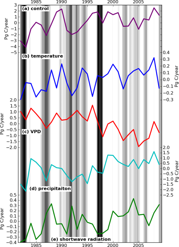
The effect of each climate component on the interannual variations of global GPP is shown in Figure 1. Under S_control, GPP kept increasing until around 2000 and then declined modestly until 2007. This trend is consistent with the results of shorter-term studies using the MODIS 17 algorithm [6,32]. For each climate variable analysis, only S_vpd showed a consistent decreasing trend, while the other simulations all produced increasing trends in global GPP (Figure 1). These results suggest that land models solely relying on VPD may overestimate the reduction in GPP caused by water stress in 2000s.
The cross-correlation coefficient matrix among the GPP time series produced by the different simulations is shown in Table 2. The GPP derived from the four climate variable simulations (S_temp, S_vpd, S_precip, and S_srad) did not correlate well with each other. The highest correlation was found between S_temp and S_precip, but the Pearson coefficient is still low (r = 0.43). Thus, the high correlation between S_clim and S_precip can be simply explained with precipitation having the strongest influence on climate-driven GPP.
In spite of the low correlation coefficients among the four climate variable simulations, Figure 1 shows a clear correspondence in the short term, i.e., shorter than a decade. S_temp and S_vpd are anti-correlated, with increases in the GPP driven by temperature and decreases in the GPP driven by VPD. The symmetric patterns are caused by VPD variation being largely driven by temperature. Elevated temperatures promote higher GPP at high latitudes, while high VPD lowers GPP by inducing drought stress.
The comparison between S_vpd and S_precip in Figure 1 showed a different correlation pattern between short and long-term. Over the short-term, as in the case of ENSO, both S_vpd and S_precip decreased. Meanwhile, over long-term, the S_vpd showed the opposite trend of S_precip. The trend of increasing temperatures caused S_vpd to have an overall decreasing trend, while S_precip increased over the same period. The controlling effects of temperature on VPD also resulted in S_vpd having no correlation with MEI (r = 0.04), while S_precip was well correlated with MEI (r = −0.79) (Table 2).
The same analysis presented in Table 2 was performed using the residual carbon flux, which was calculated from fossil fuel and cement emissions, land-use change emissions, atmospheric growth, and ocean carbon flux [36]. Assuming that the residual carbon is equivalent to the land sink, the analysis can directly assess the climate influence on carbon sequestration by land vegetation. The correlation coefficient of S_precip was improved from 0.01 to 0.31, but the correlation was still insignificant. The coefficients of the other simulations (S_clim, S_temp, S_vpd, and S_srad) were not improved.
3.2. Can Simulated Global GPP Explain Interannual Variations in Atmospheric CO2 Growth Rate?
Among the four climate component simulations, S_vpd had the highest correlation with the growth rate of CO2 (r = −0.69) (Table 2). As a first thought this high correlation could lead to validating the hypothesis that VPD controls global GPP and the CO2 growth rate. However, this hypothesis must be rejected on the grounds that the CO2 growth rate should strongly correlate with the Net Ecosystem Production (NEP). On the other hand, it has to be noted that S_vpd is strongly correlated with the GISS tropical (24°N–24°S) land temperature (r = −0.85), and the GISS tropical land temperature is also highly correlated with the CO2 growth rate (r = 0.74). It is therefore reasonable to assume that S_vpd shows a spurious and not a causal relationship with the CO2 growth rate through temperature, which controls both S_vpd and respiration.
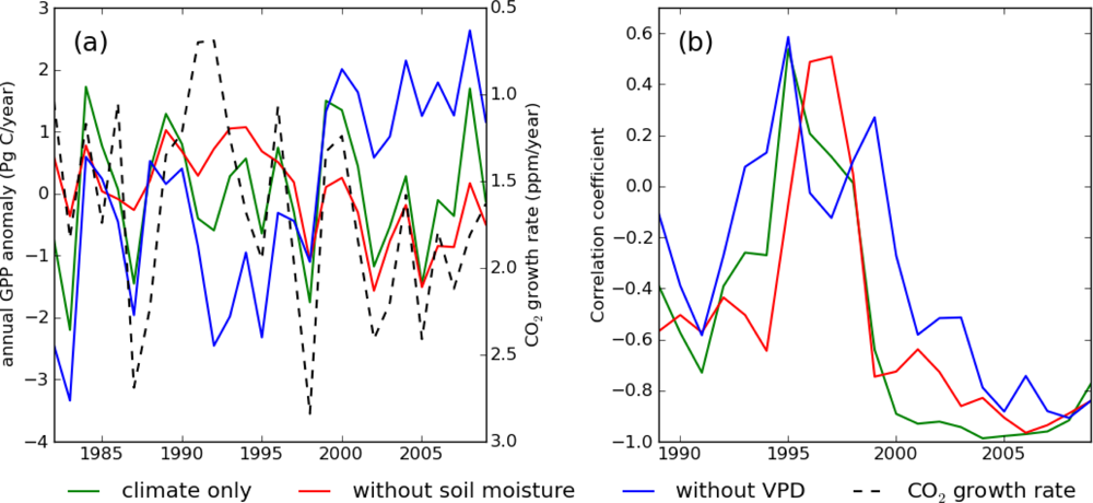
In Figure 2 we compared the time-series of S_clim, S_wo_sm, and S_wo_vpd with the CO2 growth rate. S_wo_sm and S_wo_vpd showed opposite long-term trends, more pronounced from the year 2000 onwards (Figure 2(a)), similarly to what was observed for S_vpd and S_precip in Figure 1. Overall, in the short term the interannual variations in GPP of the three simulations are anti-correlated with the CO2 growth rate. Similar to the relationship between S_precip and S_vpd, S_wo_sm showed higher correlation with the CO2 growth rate (Figure 2(b)). The long-term correlation coefficients of S_wo_sm and S_wo_vpd with the CO2 growth rate were −0.67 and 0.12, respectively. However, in the Pinatubo eruption era (1991–1994), all the three simulations deviated from the CO2 growth rate. This confirms that one cannot explain the CO2 growth rate variability through GPP variability and that changes in respiration are required to simulate the observed CO2 growth rate. Therefore, though we still cannot exclude the possibility that TOPS failed to model VPD drought-effect on GPP, high correlation between GPP and CO2 growth rate was most likely spurious. Increase in diffusive radiation ratio in Pinatubo eruption era can mitigate the reduction in global GPP, but the effect was not strong enough to make global GPP increase [37].
3.3. Which Control (VPD or Soil Moisture) Can Explain Long-Term Trend in GIMMS NDVI?
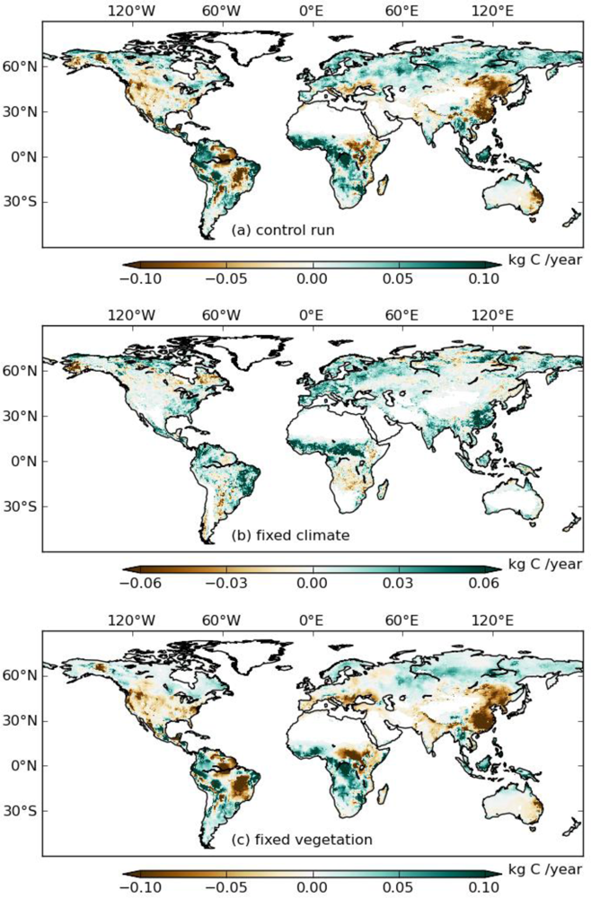
To evaluate whether the TOPS simulations are consistent with satellite observations, we calculated the differences of mean annual GPP between 2000–2009 and 1982–1999 for three simulations (S_control, S_veg, and S_clim) (Figure 3). Because S_veg was derived from GIMMS 3g under a fixed climate, we can assume S_veg to correspond to the anomaly of satellite-observed GPP. S_control and S_clim were very consistent with each other, while S_veg showed spatial patterns of higher GPP in China, Brazil, India, and USA, indicating that TOPS underestimated GPP in these regions during the 2000s.
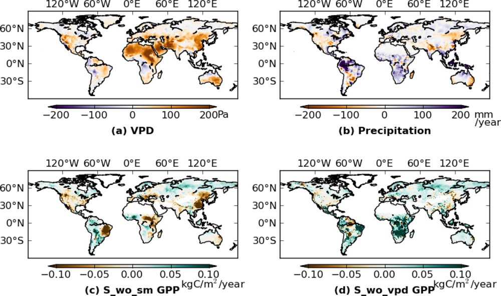
Next, we calculated the difference of mean annual GPP between 2000–2009 and 1982–1999 for S_wo_sm and S_wo_vpd (Figure 4(c,d)). Inconsistencies between S_wo_sm and S_wo_vpd occurred in Brazil, Africa, and Europe, with S_wo_sm showing more negative anomalies than S_wo_vpd in most of the regions. In these regions, precipitation increased in 2000s (Figure 4(b)), while VPD also increased (Figure 4(a)). Estimates from S_wo_vpd, compared to S_wo_sm, are more consistent with S_veg (Figure 3(b)) especially in West Brazil and Europe. Overall the effects of drought stress were more marked in the S_wo_sm simulations than in S_wo_vpd.
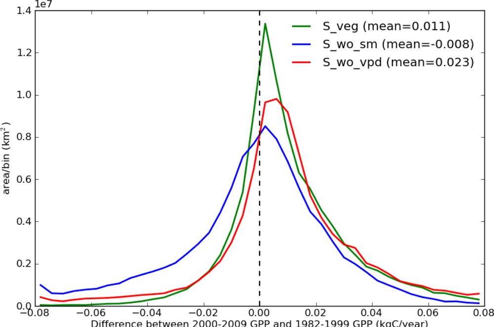
Figure 5 shows the histograms of the differences between 2000–2009 GPP and 1982–1999 GPP for the 3 simulations (S_veg, S_wo_sm, and S_wo_vpd), which were derived from Figures 3(b) and 4. Both S_veg and S_wo_vpd were positively skewed (skewness are 0.597 and 1.865, respectively), while S_wo_sm was negatively skewed (skewness is −1.460). The mean of S_veg (0.011 kg·C·yr−1) was between the means of S_wo_sm (−0.008 kg·C·yr−1) and S_wo_vpd (0.023 kg·C·yr−1). As a result, distribution of S_veg is between S_wo_vpd and S_wo_sm, but closer to S_wo_vpd than S_wo_sm. These results suggest that the TOPS model overestimated the drought stress due to an overestimated VPD effect in the 2000s, and that both precipitation and VPD down regulation functions are required to simulate the long-term GPP trend.
4. Discussion
According to van der Molen et al.[38], there are two direct dependencies of GPP on drought: structural changes in the vegetation, and physiological responses of the vegetation. In this study we only consider the latter ones. Depending on the physiological responses of stomata to soil moisture, plant species can be roughly divided into two types, i.e., isohydric and anisohydric species [39]. The isohydric species close their stomata when soil moisture decreases or VPD increases, while the anisohydric species are insensitive to soil moisture but close their stomata only responding to high VPD. Therefore, modeling drought response using VPD or soil moisture is similar to assuming that vegetation is composed by either isohydric or anisohydric species. The TOPS model structure assumes an isohydric behavior of vegetation, whereas models in which drought is simulated through VPD controls, such as the MODIS 17 algorithm, assume an anisohydric behavior of vegetation. Although plants cannot be clearly divided into isohydric or anisohydric by species [40], forest trees are predominantly of isohydric nature [41–43]. Thus, ecosystem models should have both VPD and soil moisture sub-models to properly represent the drought effect on GPP.
Although both VPD and precipitation are required for modeling physiological processes an exception can be made for short-term analyses when VPD and precipitation tend to be closely related. Our simulation in Figure 1 showed similar trend with MODIS17 analysis in 2000s [6]. Caution should be exerted, however, in extending the interpretation of short-term effects of drought effects on GPP to long-term trends. Our 30-year simulation clearly showed different trends between soil moisture-driven and VPD-driven simulations. Dynamic global vegetation models (DGVMs) also showed model-dependent sensitivities to increased VPD in correspondence to increased temperature in the Amazon during the 21st century [44].
Though this study focused on the global scale variability and trends in GPP, we need more studies dealing with the differential controls on a regional scale. For example, Mu et al.[11] reported the decoupling between precipitation and VPD caused a failure in GPP simulation by MODIS 17 algorithm in monsoon-controlled China. It is also known that variations in VPD sometimes fail to capture severe droughts at a watershed scale [45]. Therefore, assessing long-term trend in GPP in regional scale is more difficult by VPD-only model.
In addition to climate variability, other factors, not accounted here, such as CO2 fertilization, nitrogen deposition [46], and diffuse radiation [37], affect the interannual variation in GPP. These effects are difficult to quantify and complicate the bottom-line GPP trend through combined effects [47]. In this study, by focusing on the difference of after-2000 and before-2000, we ignored these effects on the interannual variation in GPP. CO2 concentration and nitrogen deposition have a smaller interannual variability compared to the climate variables [5,48], and the effect of diffuse radiation is marginal over the three decades studied here [37].
The differences in GPP after 2,000 simulated by different models were also found in time series of estimated evapotranspiration [49]. Jung et al.[49] showed that most of the ecosystem models displayed an increasing trend in modeled evapotranspiration from 1982 to 1998, but after that trends diverged among models. Jung et al.[49] concluded that the decreasing trend in evapotranspiration found in some models after 1998 was due to the limited soil moisture supply. However, similarly to the divergent GPP trends simulated for the 2000s, the diversion after 1998 can be explained by the relative sensitivity of the model structure to VPD compared to other climate components. The observed global warming trend over the past few decades causes the VPD to increase. It is therefore crucial to assess how different land models handle drought stress so as not to equate an increasing trend in VPD with a decline in GPP or ET.
This study focused on long-term trend around three decades, so that this study does not provide any conclusive judgment on the topic of short-term drought-induced NPP decline after 2000 [6,50,51]. Furthermore, discussing NPP trend is harder than GPP because of the need to include autotrophic respiration which is complex in itself [7]. Our results suggest that proper assessment of water limitation is one of the key issues to be clarified before assessing trends in global GPP or NPP.
5. Conclusions
In this study we performed a series of experiments using the TOPS model and Global Inventory Modeling and Mapping Studies (GIMMS) 3g data to evaluate the impacts of drought on the interannual variation of Gross Primary Production (GPP) simulated either in terms of VPD or soil moisture effects. Although Vapor Pressure Deficit (VPD) alone can simulate the effects of drought stress on GPP for short periods, we find that both VPD and soil moisture are required to simulate the long-term trend in global GPP. Terrestrial Observation and Prediction System (TOPS) simulations with a VPD control only underestimate GPP during the period 2000–2009 because of over-sensitivity to VPD drought effects. We also find that the strong correlation of the interannual variations of VPD with the CO2 growth rate observed in recent studies can be spurious because it is induced by a warming temperature trend. We recommend that assessments similar to the ones carried out for this study be performed for all ecosystem models aiming at analyzing the long-term trend in GPP or evapotranspiration. These sensitivity analyses are needed to correctly project the effects of climate change on the global carbon cycle.
Acknowledgments
We wish to thank Compton J. Tucker, Jorge E. Pinzon, and Molly E. Brown for providing GIMMS 3g datasets. This study was funded by NASA’s Earth Sciences Program. This research was performed using NASA Earth Exchange. NEX combines state-of-the-art supercomputing, Earth system modeling, remote sensing data from NASA and other agencies, and a scientific social networking platform to deliver a complete work environment in which users can explore and analyze large Earth science data sets, run modeling codes, collaborate on new or existing projects, and share results within and/or among communities.
References and Notes
- Beer, C.; Reichstein, M.; Tomelleri, E.; Ciais, P.; Jung, M.; Carvalhais, N.; Rödenbeck, C.; Arain, M.A.; Baldocchi, D.; Bonan, G.B.; et al. Terrestrial gross carbon dioxide uptake: Global distribution and covariation with climate. Science 2010, 329, 834–838. [Google Scholar]
- Ito, A. A historical meta-analysis of global terrestrial net primary productivity: Are estimates converging? Glob. Change Biol 2011, 17, 3161–3175. [Google Scholar]
- Randerson, J.T.; Chapin, F.S.; Harden, J.W.; Neff, J.C.; Harmon, M.E. Net ecosystem production: A comprehensive measure of net carbon accumulation by ecosystems. Ecol. Appl 2002, 12, 937–947. [Google Scholar]
- Denman, K.L.; Brasseur, G.; Chidthaisong, A.; Ciais, P.; Cox, P.M.; Dickinson, R.E.; Hauglustaine, D.; Heinze, C.; Holland, E.; Jacob, D.; et al. Couplings Between Changes in the Climate System and Biogeochemistry. In Climate Change 2007: The Physical Science Basis. Contribution of Working Group I to the Fourth Assessment Report of the Intergovernmental Panel on Climate Change; Solomon, S., Qin, D., Manning, M., Chen, Z., Marquis, M., Averyt, K.B., Tignor, M., Miller, H.L., Eds.; Cambridge University Press: Cambridge, UK/New York, NY, USA, 2007. [Google Scholar]
- Le Quéré, C.; Raupach, M.R.; Canadell, J.G.; Marland, G.; Bopp, L.; Ciais, P.; Conway, T.J.; Doney, S.C.; Feely, R.A.; Foster, P.; et al. Trends in the sources and sinks of carbon dioxide. Nat. Geosci 2009, 2, 831–836. [Google Scholar]
- Zhao, M.; Running, S.W. Drought-induced reduction in global terrestrial net primary production from 2000 through 2009. Science 2010, 329, 940–943. [Google Scholar]
- Potter, C.; Klooster, S.; Genovese, V. Net primary production of terrestrial ecosystems from 2000 to 2009. Clim. Change 2012, 113, 1–13. [Google Scholar]
- Ruimy, A.; Kergoat, L.; Bondeau, A. Participants of the Potsdam NPP Model Intercomparison. Comparing global models of terrestrial net primary productivity (NPP): Analysis of differences in light absorption and light-use efficiency. Glob. Change Biol 1999, 5, 56–64. [Google Scholar]
- Wang, W.; Dungan, J.; Hashimoto, H.; Michaelis, A.R.; Milesi, C.; Ichii, K.; Nemani, R.R. Diagnosing and assessing uncertainties of terrestrial ecosystem models in a multimodel ensemble experiment: 2. Carbon balance. Glob. Change Biol 2011, 17, 1367–1378. [Google Scholar]
- Churkina, G.; Running, S.W.; Schloss, A.L. The participants of the Potsdam intercomparison comparing global models of terrestrial net primary productivity (NPP): The importance of water availability. Glob. Change Biol 1999, 5, 46–55. [Google Scholar]
- Mu, Q.; Zhao, M.; Heinsch, F.A.; Liu, M.; Tian, H.; Running, S.W. Evaluating water stress controls on primary production in biogeochemical and remote sensing based models. J. Geophys. Res 2007, 112, G01012. [Google Scholar]
- Smith, T.M.; Yin, X.; Gruber, A. Variations in annual global precipitation (1979–2004), based on the Global Precipitation Climatology Project 2.5° analysis. Geophys. Res. Lett 2006, 33, L06705. [Google Scholar]
- Zhou, Y.P.; Xu, K.-M.; Sud, Y.C.; Betts, A.K. Recent trends of the tropical hydrological cycle inferred from Global Precipitation Climatology Project and International Satellite Cloud Climatology Project data. J. Geophys. Res 2011, 116, D09101. [Google Scholar]
- Fischer, E.M.; Knutti, R. Robust projections of combined humidity and temperature extremes. Nat. Clim. Chang 2012, 3, 126–130. [Google Scholar]
- Meehl, G.A.; Stocker, T.F.; Collins, W.D.; Friedlingstein, P.; Gaye, A.T.; Gregory, J.M.; Kitoh, A.; Knutti, R.; Murphy, J.M.; Noda, A.; et al. Global Climate Projections. In Climate Change 2007: The Physical Science Basis. Contribution of Working Group I to the Fourth Assessment Report of the Intergovernmental Panel on Climate Change; Solomon, S., Qin, D., Manning, M., Chen, Z., Marquis, M., Averyt, K.B., Tignor, M., Miller, H.L., Eds.; Cambridge University Press: Cambridge, UK/New York, NY, USA, 2007. [Google Scholar]
- Nemani, R.; Hashimoto, H.; Votava, P.; Melton, F.; Wang, W.; Michaelis, A.; Mutch, L.; Milesi, C.; Hiatt, S.; White, M. Monitoring and forecasting ecosystem dynamics using the Terrestrial Observation and Prediction System (TOPS). Remote Sens. Environ 2009, 113, 1497–1509. [Google Scholar]
- Monteith, J. Solar radiation and productivity in tropical ecosystems. J. Appl. Ecol 1972, 9, 747–766. [Google Scholar]
- Jarvis, P.G. The interpretation of the variations in leaf water potential and stomatal conductance found in canopies in the field. Phil. Trans. R. Soc. Lond. B Bio. Sci 1976, 273, 593–610. [Google Scholar]
- Running, S.W.; Hunt, E.R., Jr. Generalization of a Forest Ecosystem Process Model for Other Biomes, Biome-BGC, and an Application for Global-Scale Models. In Scaling Physiological Processes: Leaf to Globe; Ehleringer, J.R., Field, C.B., Eds.; Academic Press: San Diego, CA, USA, 1993; pp. 141–158. [Google Scholar]
- Ichii, K.; White, M.A.; Votava, P.; Michaelis, A.; Nemani, R.R. Evaluation of snow models in terrestrial biosphere models using ground observation and satellite data: Impact on terrestrial ecosystem processes. Hydrol. Process 2008, 22, 347–355. [Google Scholar]
- Nemani, R.; White, M.; Pierce, L.; Votava, P.; Coughlan, J.; Running, S. Biospheric monitoring and ecological forecasting. Earth Obs. Mag. 2003, 3/4, 6–8. [Google Scholar]
- Oren, R.; Sperry, J.S.; Katul, G.G.; Pataki, D.E.; Ewers, B.E.; Phillips, N.; Schäfer, K.V.R. Survey and synthesis of intra- and interspecific variation in stomatal sensitivity to vapour pressure deficit. Plant Cell Environ 1999, 22, 1515–1526. [Google Scholar]
- Reichstein, M. Inverse modeling of seasonal drought effects on canopy CO2/H2O exchange in three Mediterranean ecosystems. J. Geophys. Res 2003, 108, 4726. [Google Scholar]
- Zhao, M.; Heinsch, F.A.; Nemani, R.R.; Running, S.W. Improvements of the MODIS terrestrial gross and net primary production global data set. Remote Sens. Environ 2005, 95, 164–176. [Google Scholar]
- Zhu, Z.C.; Bi, J.; Pan, Y.; Ganguly, S.; Anav, A.; Xu, L.; Samanta, A.; Piao, S.; Nemani, R.R.; Myneni, R.B. Global data sets of vegetation LAI3g and FPAR3g derived from GIMMS NDVI3g for the period 1981 to 2011. Remote Sens 2013, 5, 927–948. [Google Scholar]
- Friedl, M.A.; Sulla-Menashe, D.; Tan, B.; Schneider, A.; Ramankutty, N.; Sibley, A.; Huang, X. MODIS collection 5 global land cover: Algorithm refinements and characterization of new datasets. Remote Sens. Environ 2010, 114, 168–182. [Google Scholar]
- CRUNCEP Data Set. Available online: http://dods.extra.cea.fr/data/p529viov/cruncep/readme.htm (accessed on 13 June 2012).
- University of East Anglia Climatic Research Unit (CRU), CRU Time Series (TS) High Resolution Gridded Datasets. Climatic Research Unit (CRU) Time-Series Datasets of Variations in Climate with Variations in Other Phenomena. Available online: http://badc.nerc.ac.uk/view/badc.nerc.ac.uk__ATOM__dataent_1256223773328276 (accessed on 13 June 2012).
- Kalnay, E.; Kanamitsu, M.; Kistler, R.; Collins, W.; Deaven, D.; Gandin, L.; Iredell, M.; Saha, S.; White, G.; Woollen, J.; et al. The NCEP/NCAR 40-year reanalysis project. Bull. Am. Meteorol. Soc 1996, 77, 437–471. [Google Scholar]
- Abbott, P.F.; Tabony, R.C. The estimation of humidity parameters. The Meteorol. Mag 1985, 114, 49–56. [Google Scholar]
- Ichii, K.; Hashimoto, H.; Nemani, R.; White, M. Modeling the interannual variability and trends in gross and net primary productivity of tropical forests from 1982 to 1999. Glob. Planet. Change 2005, 48, 274–286. [Google Scholar]
- Nemani, R.R.; Keeling, C.D.; Hashimoto, H.; Jolly, W.M.; Piper, S.C.; Tucker, C.J.; Myneni, R.B.; Running, S.W. Climate-driven increases in global terrestrial net primary production from 1982 to 1999. Science 2003, 300, 1560–1563. [Google Scholar]
- Conway, T.; Tans, P. Trends in Atmospheric Carbon Dioxide. Available online: www.esrl.noaa.gov/gmd/ccgg/trends/ (accessed on 13 June 2012).
- Wolter, K.; Timlin, M.S. El Niño/Southern Oscillation behaviour since 1871 as diagnosed in an extended multivariate ENSO index (MEI.ext). Int. J. Climatol 2011, 31, 1074–1087. [Google Scholar]
- Hansen, J.; Ruedy, R.; Sato, M.; Imhoff, M.; Lawrence, W.; Easterling, D.; Peterson, T.; Karl, T. A closer look at United States and global surface temperature change. J. Geophys. Res 2001, 106, 23947–23963. [Google Scholar]
- Le Quéré, C.; Andres, R.J.; Boden, T.; Conway, T.; Houghton, R. A.; House, J. I.; Marland, G.; Peters, G. P.; van der Werf, G.; Ahlström, A.; et al. The global carbon budget 1959–2011. Earth Syst. Sci. Data Discuss 2012, 5, 1107–1157. [Google Scholar]
- Mercado, L.M.; Bellouin, N.; Sitch, S.; Boucher, O.; Huntingford, C.; Wild, M.; Cox, P.M. Impact of changes in diffuse radiation on the global land carbon sink. Nature 2009, 458, 1014–1017. [Google Scholar]
- Van der Molen, M.K.; Dolman, A.J.; Ciais, P.; Eglin, T.; Gobron, N.; Law, B.E.; Meir, P.; Peters, W.; Phillips, O.L.; Reichstein, M.; et al. Drought and ecosystem carbon cycling. Agr. Forest Meteorol 2011, 151, 765–773. [Google Scholar]
- Tardieu, F.; Simonneau, T. Variability among species of stomatal control under fluctuating soil water status and evaporative demand: Modelling isohydric and anisohydric behaviours. J. Exp. Bot 1998, 49, 419–432. [Google Scholar]
- Franks, P.J.; Drake, P.L.; Froend, R.H. Anisohydric but isohydrodynamic: Seasonally constant plant water potential gradient explained by a stomatal control mechanism incorporating variable plant hydraulic conductance. Plant Cell Environ 2007, 30, 19–30. [Google Scholar]
- Bucci, S.J.; Goldstein, G.; Meinzer, F.C.; Franco, A.C.; Campanello, P.; Scholz, F.G. Mechanisms contributing to seasonal homeostasis of minimum leaf water potential and predawn disequilibrium between soil and plant water potential in Neotropical savanna trees. Trees 2005, 19, 296–304. [Google Scholar]
- Fisher, R.A.; Williams, M.; Do Vale, R.L.; Da Costa, A.L.; Meir, P. Evidence from Amazonian forests is consistent with isohydric control of leaf water potential. Plant Cell Environ 2006, 29, 151–165. [Google Scholar]
- Bond, B.J.; Meinzer, F.C.; Brooks, J.R. Chapter 2. How Trees Influence the Hydrological Cycle in Forest Ecosystems. In Hydroecology and Ecohydrology: Past, Present and Future; Wood, P.J., Hannah, D.M., Sadler, J.P., Eds.; John Wiley & Sons Ltd: West Sussex, UK, 2008; pp. 7–35. [Google Scholar]
- Galbraith, D.; Levy, P.E.; Sitch, S.; Huntingford, C.; Cox, P.; Williams, M.; Meir, P. Multiple mechanisms of Amazonian forest biomass losses in three dynamic global vegetation models under climate change. New Phytol 2010, 187, 647–65. [Google Scholar]
- Hwang, T.; Kang, S.; Kim, J.; Kim, Y.; Lee, D.; Band, L. Evaluating drought effect on MODIS Gross Primary Production (GPP) with an eco-hydrological model in the mountainous forest, East Asia. Glob. Change Biol 2008, 14, 1037–1056. [Google Scholar]
- Reich, P.B.; Hobbie, S.E.; Lee, T.; Ellsworth, D.S.; West, J.B.; Tilman, D.; Knops, J.M.H.; Naeem, S.; Trost, J. Nitrogen limitation constrains sustainability of ecosystem response to CO2. Nature 2006, 440, 922–925. [Google Scholar]
- McMurtrie, R.E.; Norby, R.J.; Medlyn, B.E.; Dewar, R.C.; Pepper, D.A.; Reich, P.B.; Barton, C.V.M. Why is plant-growth response to elevated CO 2 amplified when water is limiting, but reduced when nitrogen is limiting? A growth-optimisation hypothesis. Funct. Plant Biol 2008, 35, 521. [Google Scholar]
- Reay, D.S.; Dentener, F.; Smith, P.; Grace, J.; Feely, R.A. Global nitrogen deposition and carbon sinks. Nat. Geosci 2008, 1, 430–437. [Google Scholar]
- Jung, M.; Reichstein, M.; Ciais, P.; Seneviratne, S.I.; Sheffield, J.; Goulden, M.L.; Bonan, G.; Cescatti, A.; Chen, J.; De Jeu, R.; et al. Recent decline in the global land evapotranspiration trend due to limited moisture supply. Nature 2010, 467, 951–954. [Google Scholar]
- Samanta, A.; Costa, M.H.; Nunes, E.L.; Vieira, S.A.; Xu, L.; Myneni, R.B. Comment on “Drought-induced reduction in global terrestrial net primary production from 2000 through 2009”. Science 2011, 333, 1093, author reply 1093. [Google Scholar]
- Medlyn, B.E. Comment on “Drought-induced reduction in global terrestrial net primary production from 2000 through 2009”. Science 2011, 333, 1093, author reply 1093. [Google Scholar]


| LAI/FPAR | Temperature | VPD | Precipitation | Radiation | Model | |
|---|---|---|---|---|---|---|
| S_control | x | x | x | x | x | |
| S_veg | x | |||||
| S_clim | x | x | x | x | ||
| S_temp | x | |||||
| S_vpd | x | |||||
| S_precip | x | |||||
| S_srad | x | |||||
| S_wo_vpd | x | x | x | x | ΨVPD = 1 | |
| S_wo_sm | x | x | x | x | ΨSM = 1 |
| S_clim | S_temp | S_vpd | S_precip | S_srad | CO2 | MEI | GISS | |
|---|---|---|---|---|---|---|---|---|
| S_clim | -- | 0.25 | 0.48 | 0.70 | 0.15 | −0.49 | −0.73 | −0.25 |
| S_temp | 0.25 | -- | −0.39 | 0.43 | 0.37 | 0.29 | −0.35 | 0.55 |
| S_vpd | 0.48 | −0.39 | -- | −0.21 | −0.35 | −0.69 | −0.04 | −0.87 |
| S_precip | 0.70 | 0.43 | −0.21 | -- | 0.37 | 0.01 | −0.79 | 0.37 |
| S_srad | 0.15 | 0.37 | −0.35 | 0.37 | -- | 0.18 | −0.19 | 0.41 |
Share and Cite
Hashimoto, H.; Wang, W.; Milesi, C.; Xiong, J.; Ganguly, S.; Zhu, Z.; Nemani, R.R. Structural Uncertainty in Model-Simulated Trends of Global Gross Primary Production. Remote Sens. 2013, 5, 1258-1273. https://0-doi-org.brum.beds.ac.uk/10.3390/rs5031258
Hashimoto H, Wang W, Milesi C, Xiong J, Ganguly S, Zhu Z, Nemani RR. Structural Uncertainty in Model-Simulated Trends of Global Gross Primary Production. Remote Sensing. 2013; 5(3):1258-1273. https://0-doi-org.brum.beds.ac.uk/10.3390/rs5031258
Chicago/Turabian StyleHashimoto, Hirofumi, Weile Wang, Cristina Milesi, Jun Xiong, Sangram Ganguly, Zaichun Zhu, and Ramakrishna R. Nemani. 2013. "Structural Uncertainty in Model-Simulated Trends of Global Gross Primary Production" Remote Sensing 5, no. 3: 1258-1273. https://0-doi-org.brum.beds.ac.uk/10.3390/rs5031258