Characterization of Canopy Layering in Forested Ecosystems Using Full Waveform Lidar

Abstract

Canopy structure, the vertical distribution of canopy material, is an important element of forest ecosystem dynamics and habitat preference. Although vertical stratification, or “canopy layering,” is a basic characterization of canopy structure for research and forest management, it is difficult to quantify at landscape scales. In this paper we describe canopy structure and develop methodologies to map forest vertical stratification in a mixed temperate forest using full-waveform lidar. Two definitions—one categorical and one continuous—are used to map canopy layering over Hubbard Brook Experimental Forest, New Hampshire with lidar data collected in 2009 by NASA’s Laser Vegetation Imaging Sensor (LVIS). The two resulting canopy layering datasets describe variation of canopy layering throughout the forest and show that layering varies with terrain elevation and canopy height. This information should provide increased understanding of vertical structure variability and aid habitat characterization and other forest management activities.

1. Introduction

The function and diversity of forest ecosystems are dependent on the physical structure of the vegetation [1,2]. Canopy structure, the distribution of plant material within the canopy, can vary as a function of stand age and environmental factors [3] and affects species diversity, plant growth, and other aspects of the forest ecosystem [1–4]. Ecologists have long noted that vertical structure can account for patterns of animal diversity and richness [1,5], and have suggested a mechanism of niche partitioning along the vertical axis (e.g., [6]). Structure and arrangement of canopy layers is also an important component of species habitat suitability, and maps of vertical structure will aid in forest management strategies [2]. Here, we examine the vertical distribution of material within the canopy and develop methodologies that quantify canopy layering in order to examine how it varies horizontally.

Traditional stratification studies have historically been based on field data, relying on sparse sampling within the forest study area. Hand-drawn canopy profiles are often used to depict vertical stratification [7–9], and numerical algorithms have also been used to evaluate layering within field-measured canopy [3,10,11]. Both of these analyses are limited to the scale of a sample plot and are subjective in their interpretation. Field-based measurements of vertical forest structure are time-consuming and cannot be practically obtained over large areas, which limit the usefulness of the data when applied to larger areas [12]. Moreover, there is no consensus about the best measurement strategy, and a vast range of metrics have been proposed by foresters and researchers for depicting and analyzing the distribution of forest canopy along the vertical axis, especially for canopy layering or vertical stratification [9,11,13,14]. For example, the varying definitions of canopy layering include inconsistent vertical vegetation distribution [15], differing levels of individual tree height [16–18], aggregation of tree species [16], and vertical foliage distribution [13]. Thus, our ability to both fully understand and compare canopy layering between different forested ecosystems has been limited.

Light detecting and ranging (lidar) remote sensing is an ideal technology to detect layering within the vertical canopy structure. This active form of remote sensing provides information on the 3-D structure of forest canopies by transmitting laser pulses that are then reflected by canopy elements, showing not only height but also the structure within the canopy from the top to the forest floor [19–21]. Both discrete-return and waveform lidar have been used in many different ecosystems to retrieve elements of forest structure, including canopy height, biomass, and various parameters related to the vertical distribution of leaves and branches (e.g., canopy closure, LAI, canopy height profile, and vertical foliar diversity) [19,20,22–24].

Numerous lidar-derived products, such as canopy height, canopy cover, canopy complexity, and foliar height diversity, have been shown to accurately depict canopy elements essential for habitat suitability and forest management at the landscape scale [22,24–26]. Lidar-derived canopy cover is comparable to field-based estimates [12,22,27,28] and has been used as a forest descriptor for research in forest structure and species habitat [20,24,29,30]. Similarly, the lidar-derived apparent foliage area profile has been used in numerous forest structure studies, providing useful information on forest structure that is comparable to physical measurements [31,32].

While some remote sensing studies (usually using discrete return small footprint lidar) have specifically considered vertical stratification, they have not produced a consistent remote-sensing methodology for determining layering within the canopy [18,33–36]. The number of returns within subjectively determined canopy layers has served as inputs for habitat models [34,36]. Clawges et al.[34] suggest that the amount of vegetation within specific layers impacts the habitat suitability for certain avian species. Similarly, Swatantran et al.[24] suggested stratification in Hubbard Brook Experimental Forest based on bird habitat preferences for canopy cover at different height levels. However, these results have not been translated into ecologically meaningful terms, such as number of canopy layers or a consistent metric for vertical stratification. Movement towards reconciliation of these new, remotely sensed metrics with more familiar ground measurements provides researchers and forest managers a link by which they can apply landscape scale measurements of vertical structure variability to problems of habitat and forest management that have been severely constrained by lack of data.

Thus, to more fully understand the role of vertical canopy structure in forest dynamics and species habitat, methodologies must be developed that bridge the gap between lidar remote sensing technology and ecological research and conservation application. Basing lidar metrics on variables understood in forestry and ecological research should result in more meaningful information and methodologies that can be applied across ecosystems [36]. Once this is accomplished, an exploration of factors affecting the spatial variability of vertical canopy structure may lead to important generalizations and insights applicable across ecosystems.

The goal of our research is to characterize the vertical canopy structure in the mixed deciduous forest of Hubbard Brook Experimental Forest (HBEF) and examine the vertical distribution of canopy material using full waveform lidar. In particular, we seek to explore methods for mapping the spatial distribution of vertical canopy layering. First we describe our study area and the lidar data acquisitions over it. Next, we characterize the vertical structure of foliage throughout HBEF. We then outline two methods for depicting vertical structure: the first is based on categorization of structure into nine types, and the second uses the continuous foliage profile to find significant concentrations of vertical canopy material. We then apply both methods to produce spatial maps of layering across the HBEF watershed and explore whether spatial patterns in structure are related to gradients in two factors hypothesized to affect layering, canopy height and terrain elevation, both of which vary greatly within the study area (Figure 1). Lastly, we discuss in detail potential sources of variation in our maps and the type of information provided by each layering dataset.

2. Material and Methods

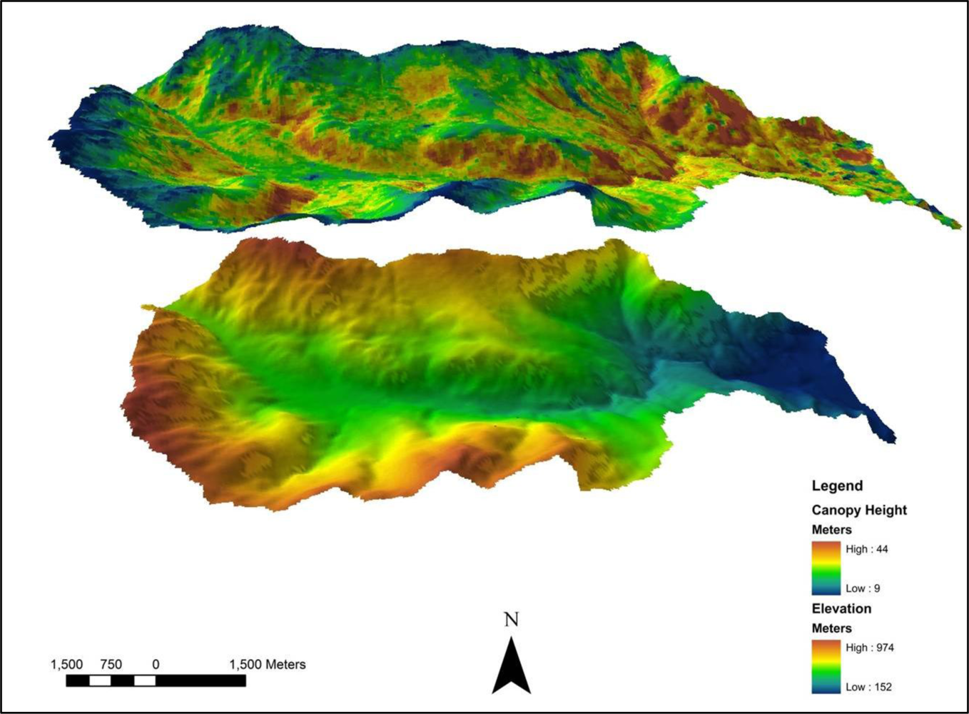
2.1. Study Area

The study area covers 3,185 ha of the White Mountain National Forest, including Hubbard Brook Experimental Forest, and is located in central New Hampshire, USA. The forest resides in an east-west oriented watershed (Figure 2). Elevation within HBEF ranges from 220 m to 1,015 m above sea level. The canopy is predominately red spruce (Picea rubens), balsam fir (Abies balsamica), and birch (Betula sp.) at higher elevations and sugar maple (Acer saccharum) and beech (Fagus grandiflora) at lower elevations [37].

2.2. Lidar Data

Waveform lidar was acquired over HBEF in the summer of 2009 from the Laser Vegetation Imaging Sensor (LVIS). LVIS is a medium-footprint, full-waveform lidar developed at NASA’s Goddard Space Flight Center [38]. LVIS records the entire outgoing and return signal to provide waveforms that can be used to map sub-canopy topography, canopy height and vertical foliage profiles. The amplitude of the geolocated waveform at a given height is proportional to the amount of canopy material at that height making it suitable for canopy stratification studies [22]. LVIS was flown at an altitude that achieved a nominal 25-m diameter footprint on the ground. The footprints overlap slightly in the across- and along-track flight direction to achieve approximately contiguous coverage over the entire imaging swath (about 2 km wide for these flights). A detailed description of LVIS waveform processing is available in Hofton et al.[39] and Dubayah et al.[40].

High slopes within the study area can sometimes affect the ability of LVIS algorithms to accurately determine ground returns (see [40]). While such errors are generally small, they can be as much as a few meters for isolated shots, the effect of which provides an inaccurate estimate of elevation for that observation, and therefore canopy height. Discrete return lidar (DRL) data also were available for HBEF, and upon comparing DRL with LVIS, we found that the DRL ground elevation measurements were more accurate. Therefore, we used the DRL data to correct LVIS ground-finding errors (following [24]). However, had there not been a noticeable issue with the LVIS ground returns for this particular set of LVIS data, the DRL measurements would not have been necessary, and the ground and canopy height measurements would have been directly derived from the LVIS data as shown for other LVIS datasets (e.g., [22,41]. DRL measurements were acquired over the area in 2009 with a return density of about 5 shots per square meter. Canopy height was calculated by subtracting average elevation of DRL within an LVIS footprint from the LVIS detected canopy top, which is the lidar return at the top of the waveform greater than the noise threshold [24] (Figure 2).

2.3. Characterization of Vertical Canopy Structure

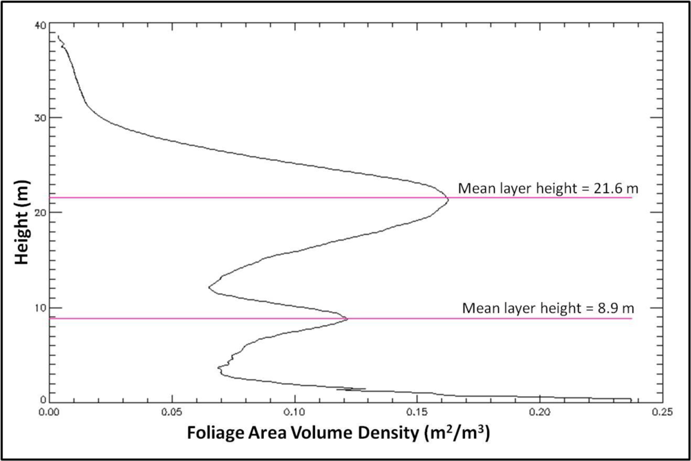
2.3.1. Foliage Area Profile

Lidar-derived apparent foliage profiles portray the vertical distribution of foliage area volume density (m²/m³) [42]. These were calculated from the LVIS waveforms based on methods used in Ni-Meister et al.[42] for LVIS lidar data flown over HBEF in 2009. Although it has been noted that in some areas (mainly coniferous forests) the apparent foliage profile can underestimate the foliage area density due to the clumping of needle leaf foliage [42]; previous studies have determined that it can still provide useful information on forest structure that is comparable to physical measurements [31,32]. The apparent foliage area was aggregated into 3-m height bins (from the ground to the top of the canopy) and then averaged over a 30 × 30-m grid for the entire forest. Due to mixing between the ground and canopy return [39] only the height intervals above 3 m were used because of potential amplification of foliage area near the ground. These profiles were then analyzed for HBEF as a whole, as well as a function of three elevation ranges. Sherry [8] examined the foliage area of HBEF between 500 and 600 m and we use this as a starting point for our stratification into low, middle, and high elevations. Our elevation levels coincide with the terrain features of the Forest, with areas of low elevation (<500 m) occurring around the major rivers and streams in the watershed, middle elevation (500 m to 700 m) occurring in the between the wetland areas and the forest edge, and areas of high elevation (>700 m) occurring around the edge of the watershed, furthest away from the riverine valleys.

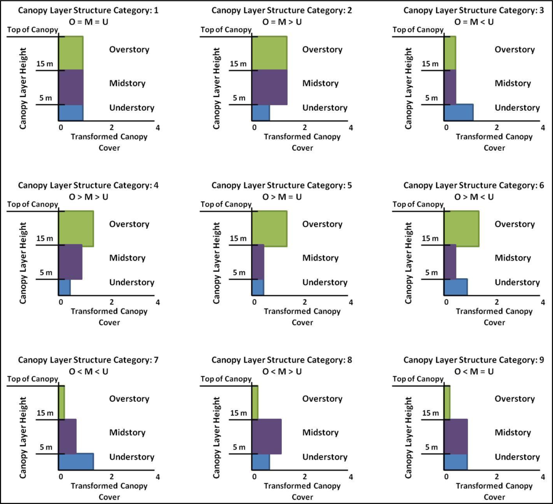
2.3.2. Canopy Layer Structure

Canopy cover in any location is defined as the amount of sky (in percent) not obscured by vegetation at nadir. Cumulative canopy cover is the summed canopy cover from the top of the canopy (zero) to the ground (total canopy cover). Lidar derived canopy cover has shown to be comparable to field based estimates [12,22,43]. The high accuracy of lidar derived canopy cover has led it to be used as a forest descriptor for research in forest structure and species habitat [24,43]. For any particular vertical segment of the canopy, the return waveform energy in that cross-section is divided by the waveform’s total return energy, which, after accounting for differences between ground and canopy reflectance, allows for the calculation of cumulative canopy cover. Cumulative canopy profiles were calculated following methods outlined in Ni-Miester et al.[42].We further applied the MacArthur-Horn transformation (− In (1 − cover(h)), where h refers to height) to account for the extinction of light as it travels through the canopy [44–47]. The cumulative profile was used to calculate transformed canopy cover (hereafter “canopy cover” for any given height interval within the canopy [24]).

We derived canopy cover for three basic canopy layers: understory, midstory, and overstory [48,49]. Similar to MacArthur and MacArthur [1] the height thresholds defining each of these layers were based on findings of avian species habitat preference in HBEF [24]. The understory layer is 0 to 5 m, which encompasses shrubs and small saplings [49,50]. The midstory, encompassing larger saplings and intermediate trees [51], is 5 to 15 m. The overstory, or upper layer of the canopy (15 m to the top of the canopy), contains more mature seed-bearing trees [48].

The waveforms were aggregated into a 30 × 30 m grid and the average transformed canopy cover for each of the 3 layers was calculated for the grid cells. These values were used to determine a canopy layer structure category (defined next) for each grid cell, providing a map of canopy layer structure within HBEF. The canopy layer structure is described by nine canopy configuration categories that are based on the canopy cover relative to the three canopy layers: understory (U), midstory (M), and overstory (O). The canopy cover is compared between the layers, with the overstory compared to the midstory and the midstory compared to the understory. The layers are considered different (either greater or lesser than each other) if there is a difference in the waveform-derived canopy cover greater than 10%. This comparison results in nine configuration categories that can be mapped (Figure 3). For example, category 4 (O > M > U) depicts an area where the percent cover in the overstory is greater than the midstory and the midstory cover is greater than that of the understory (in each case by at least 10%). The motivation for such a classification scheme is two-fold. First, it tends to mimic how a field ecologist might describe the canopy from the ground in terms of broad classes. Secondly, it takes a continuous variable (canopy cover), and transforms it into a measure of canopy organization that can be easily mapped and visualized.

2.3.3. Foliage Profile Layering

An alternate means of examining the vertical structure of the canopy is to evaluate the continuous profile of the canopy, instead of looking at sections of cumulative measurements (as in canopy layer structure). Peaks and troughs in the apparent foliage profile represent areas of increased and decreased reflection from canopy elements. Assuming that on average the reflectance of the canopy elements do not change much, the peaks of the foliage profile may be inferred to represent major concentrations of vegetation indicative of canopy layers [13,52]. To minimize the influence of noise, we first applied a Gaussian smoothing algorithm to the foliage profile, and then found its mode or area with the densest vegetation [13]. The other peaks of the smoothed foliage profile were detected using a moving window of five LVIS waveform height bins, which defined a peak at an inflection point in the smoothed foliage profile where afterward the foliage area decreased for five LVIS bins. The peaks were then compared to the mode of the foliage profile to determine if they are large enough to be an area of dense vegetation relative to the mode. We chose a relative difference of 30% as a threshold for determining that a layer occurred at the height, i.e., the peak had to be at least 30% as large as the profile mode. The amount of Gaussian smoothing, moving window size and peak definition parameters were determined by visual analysis.

The output of this algorithm provided the number of peaks for each waveform and the heights at which these peaks occur, which is the mean layer height (Figure 4). To minimize the potential for misidentification of canopy layers near the ground due to mixing between the ground and canopy return [39], only peaks occurring 3 m above the ground were selected. The number of apparent foliage area profile peaks was then mapped to depict the canopy layering across the landscape at a 30 m resolution in terms of the number of layers in a location and the height where the layers occur. To do this, a 30 m × 30 m grid was laid over the study area. The number of layers for each waveform was averaged for the number of waveforms in each grid cell. Then the averaged number of layers was rounded to the nearest whole number to obtain a measure of layering within each 30 m × 30 m grid cell. The layer heights were also examined to see where layers occurred within the canopy.

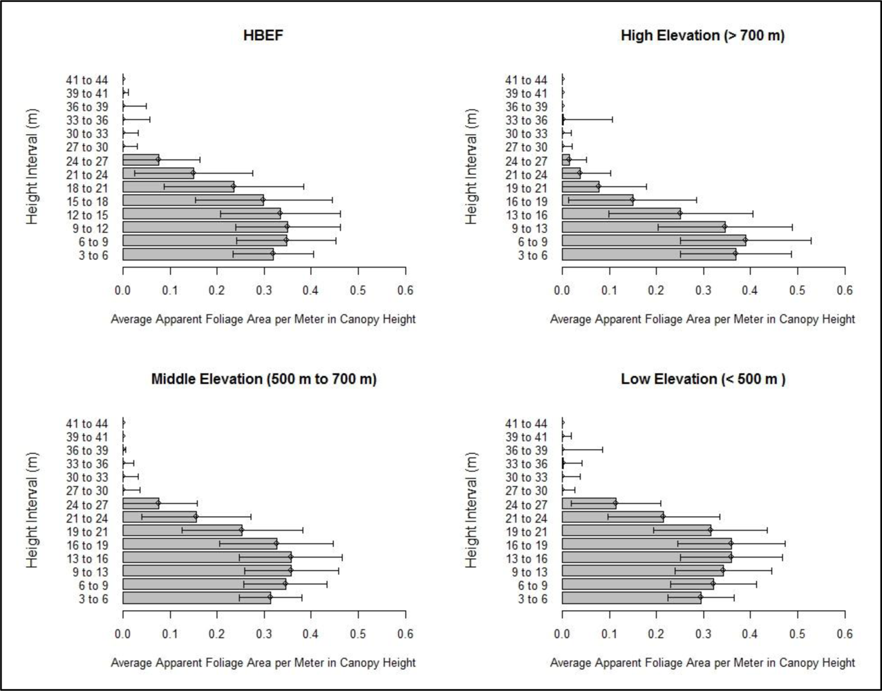
2.3.4. Height and Elevation Analyses

The results of both datasets (canopy layer structure and foliage profile layering) were mapped across HBEF. Boxplots and ANOVAS were used to evaluate how each canopy layering dataset varied with canopy height and elevation.

3. Results

3.1. Foliage Area Profile

The majority of the foliage occurred within the middle of the range of canopy heights, between 6 and 15 m (Figure 5) with an approximate peak between 9 and 12 m. This result shows that over the entire forest there is less foliage in the upper canopy. Similarly, foliage area tended to decrease towards the understory. When compared across elevation zones, the height of the peak foliage area changed. The histograms for middle and low elevations have a similar shape to that for HBEF as a whole (dominant midstory), but for high elevations the histogram is markedly different. The foliage area peaked between 6 and 9 m at high elevations but occurred higher in the canopy (between 13 and 19 m) at lower elevations (<500 m) (Figure 5). The low elevations also had the least amount of foliage at the lower part of the canopy (3 to 6 m) when compared to areas of middle and high elevation. At areas of mid elevation (500 to 700 m) the majority of the foliage area occurred between 9 and 16 m within the canopy.

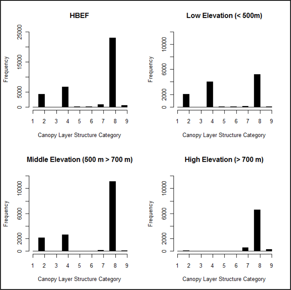
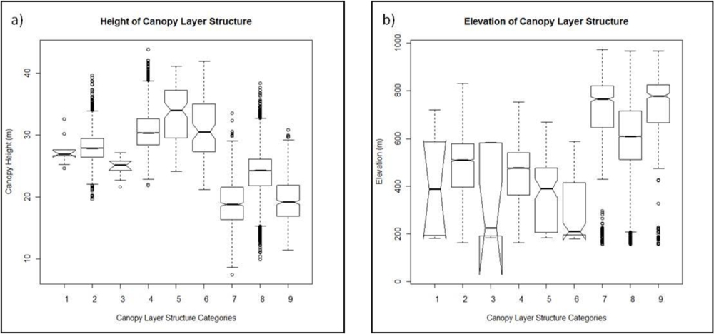
3.2. Canopy Layer Structure

All nine canopy layer structure categories were present in the Hubbard Brook Experimental Forest study area (Figure 6). Categories 2 (O = M > U) and 4 (O > M > U) (n = 4,275 and 6,680 pixels, 12% and 19% respectively) were found mainly in the forest interior, relatively close to rivers. Categories 7 and 9 (n = 875 and 472, 2.5% and 1.3%) tended to be closer to the edges of the study area. The majority of the forest fell into category 8 (O < M > U), which covers almost 2,061 ha of forest (n = 22,950 pixels, 64%) (Figure 7). These areas have a well-developed midstory and fairly open under- and overstories. The other major categories include categories 4 and 2. These results suggest that the majority of the canopy material within the forest is located in the midstory (5 to 15 m) and that in general HBEF has a fairly open understory.

The presence of specific canopy layer structure categories was related to overall canopy height and elevation based on the significant difference of median canopy height and elevation for the majority of the categories; that is, some categories were differentiated based on the median canopy height and/or median elevation of that category relative to other categories (Figure 8). These results were supported with subsequent ANOVA results (p < 0.05). However, there was a wide range both in canopy height and elevation within categories. The categories with higher average canopy heights were categories 4 (30.7 m), 5 (33.4 m) and 6 (30.9 m), all of which have dominant overstory. Categories 7, 8, and 9, which have an open overstory, occur at lower elevations, with the average elevation of 692.1 m, 598.4 m, and 713.9 m, respectively.

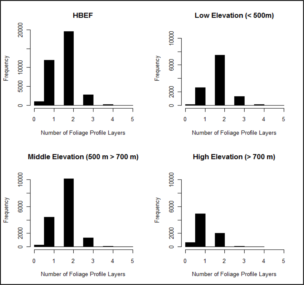
3.3. Foliage Profile Layering

The majority (55%) of the forest study area (1,762 ha) was comprised of two foliage profile layers (Figure 9), and about 34% (1,072 ha) of HBEF had one layer within the canopy. Areas with more than 3 layers accounted for less than 1% of the study area. Mapped results of the number of foliage profile layers showed that areas with 2 or more foliage profile layers tended to occur in the interior of the forest (Figure 10). Areas with one foliage profile layer were found from the edge of the forest to its interior but generally were not found in areas adjacent to rivers. Areas with 0 foliage profile layers (988 pixels in all) were generally located towards the outer edge of HBEF.

The number of foliage profile layers showed a clear, positive relationship with canopy height (Figure 11): as canopy height increases, the number of layers increases. Summary boxplots suggest a significant difference in median canopy height between most of the layer groups as well. Single-factor ANOVAs were also run between each number of foliage profile layers, confirming the significant difference (p < 0.05) in height between layers.

There was also a large range in elevation for all foliage profile layer groups (Figure 11), with the median elevation significantly different between most of the layer groups as seen in the boxplots. The conclusion that the number of layers significantly varies with elevation was confirmed with ANOVA results (p < 0.5). The areas with 0 and 1 layers, which have average elevations of 622.4 m and 711.4 m, occurred at higher elevations than those with 2 to 5 layers (ranging from 388.7 m to 523.3 m), respectively. There was a strong, negative relationship between numbers of layers and elevation. This is not surprising given the gradient in canopy height that exists at HBEF: trees are shorter as elevation increases.

When examined across all multilayer canopies (ranging from 2 to 5 layers), there was a wide range in the height of the top and bottom foliage profile layers (Figure 12). The median heights were 7 m (bottom layer) and 18 m (top layer). The height of the top layers varied with the number of layers present in the canopy and tended to increase with the number of layers identified. The lower and middle layers occurred closer together in height relative to the top layer (Figure 13).

4. Discussion

We explored how vertical canopy structure varies across HBEF using two metrics to map canopy layering derived from waveform lidar. Our results show significant spatial variability in canopy vertical structure, a result which supports previous findings of structural diversity within the forest [37]. Average foliage area profiles across elevational gradients showed differences in structure at the low, middle, and high elevation levels. Within the foliage profile, the peak in apparent foliage area decreased as elevation increased (from about 13 to 19 m at low elevations to 6 to 9 m at high elevations). Environmental gradients, such as elevation, have been repeatedly shown to have a correlation with plant growth [53–57]. These trends have also been examined within HBEF. Whittaker et al.[54] noted that there were decreasing trends in both tree height and leaf area ratio (m²/m³) with elevation in the forest. These effects could possibly be attributed to the availability of resources (such as water) or changes in climate (such as temperature) that vary along the elevational gradient, affecting tree growth [53,55–57]. In addition, disturbance may play a role. Higher elevations are more prone to the effects of wind throw, ice storms, etc., so that in addition to having slower growth rates, trees are younger at higher elevation because of repeated disturbance [58]. This finding of structural change along elevational gradients was also seen in the results from both layering data sets.

Sherry [8] used averaged foliage profiles to describe the vertical structure within a 10-ha plot in HBEF. His results showed the majority of canopy material existing around 20 m and opening dramatically from 15 m to the ground. Our results, on the other hand showed the majority of the canopy material existing lower in the canopy, between 6 and 15 m. Due to the contrast in results, we examined the change in vertical structure at differing horizontal scales, including a 9-ha area near the initial Sherry study area. We found that as the horizontal area increased, a large part of the detail in the vertical structure was lost from the foliage area profile.

Choosing a scale of analysis germane to the research goal is always important—perhaps even more so for canopy structure, as this structure is by its very nature scale-dependent. Because our data had a minimum resolution of about 25 m, we measured canopy structure as opposed to individual tree structure. The power in lidar observations is in providing structure at relatively fine resolutions while at the same time allowing for aggregations to arbitrary but ecologically significant areas. For example, while average structure for the watershed as a whole can be observed, what is more revealing is these average structures within areas where we hypothesize climatic, edaphic, and other factors may play a role in structure and its dynamics, e.g., within elevation zones, or within, say primary vs. secondary forests.

Our results showed that layering in both datasets is affected by forest growth and its impacting factors, most notably elevation. Our results corresponded with previous studies noting the effects of the elevational gradient on forest structure in HBEF [54]. For both datasets, the categories or number of layers associated with lower elevations were also the ones associated with taller canopy heights and vice versa. For the canopy layer structure dataset, these categories were categories 4, 5, and 6, which feature a more dominant overstory. This is possibly a result of tree growth and light competition, with individual canopies expanding as plants increase in height, allowing trees to receive more light for photosynthesis [59–61]. Canopy height is expected to decrease with elevation because of constraints on growth by temperature and through increased disturbance [62,63]. A taller canopy may allow more space for variations in the canopy structure to occur, resulting in more layers, especially since the top layer tends to occur higher in the canopy as the number of layers increases (Figure 13).

The foliage profile layering methodology provides a way of assessing the complexity of the canopy without relying on a priori height thresholds to determine the vertical distribution of canopy material. However, our analysis did not examine vertical structure of the canopy below 3 m. The 3-m threshold was used to avoid a potential source of error in the foliage profile algorithm caused by the mixing between the waveform ground return and the canopy return, which could inflate foliage area measurements near ground level [39]. It is thus possible that areas of dense foliage in the understory were missed in the profile layering analyses.

Given the nature of our three-layer organizational scheme for the canopy layer structure categories, we tested whether the spatially extensive occurrence of categories with a dominant midstory was an artifact of the canopy simply being less than 15 m in height. Recall that our midstory is defined as between 5 and 15 m. If the canopy is less than this height, it would lead to its frequent categorization of dominant midstory because there was no overstory. For the categories where the midstory is greater than the overstory (7, 8, and 9), only 1.45% of pixels (352 out of 24,297) had canopy heights below 15 m. Thus, the layering results are not an artifact of the classification scheme. However, in forests where canopy height is known to be short, considerations should be made when examining canopy layer structure results and care taken to choose more appropriate vertical definitions of under-, mid- and overstory heights. Indeed, the choice of layer boundary definitions is a critical aspect of the analysis, as illustrated next.

Our canopy layer structure methodology relied on literature-based height values to depict the distribution of vegetation within three distinct layers. We used height intervals that coincided with previous observations of avian species preference in HBEF. However, if the height intervals are changed, the distribution of the nine canopy layer structure categories across the landscape can change dramatically. For example, Figure 14 shows how the distribution of categories changes when the midstory height interval is changed from 5 m–15 m to 5 m–10 m. HBEF goes from a forest dominated by midstory vegetation (foliage from larger saplings and the lower portions of mature tree crowns) to a forest dominated by overstory.

That these results change is not a cause for concern, nor does it suggest a certain arbitrariness that may hinder rational insights and generalizations. Rather it highlights that, just as the choice of spatial scale is important, so too is the choice of a vertical definition. The point of using categories is to generalize structure and organization. In the absence of a priori information about logical height intervals, exploratory analyses must be used, conditioned by knowledge of the physical and biological landscape to guide what constitutes “midstory” vs. “overstory”. If extant observations conclude that a particular avian species prefers, say, an open midstory, the definition of “open midstory” is hopefully available. That it often is not, or varies by researcher, illustrates that the arbitrariness has been the rule in past analyses. We suggest that the methods presented here allow for quantitative assessments, even if definitions may vary. They are still reproducible (knowing the definition) and available at high spatial resolution across entire landscapes.

On the topic of generalization, note also that the full profile data may always be leveraged, to both validate categorizations and even help define then. For example, suppose one did not know how to choose the vertical category cut-offs (i.e., 5–15 m, etc.). One could look at the full foliage area profiles to address this issue. Figure 15 shows a few foliage area profiles from category 6, which has an open midstory from 5 to 15 m. In these examples, there is more foliage area above 15 m and below 5 m than within the midstory height interval, which supports our choice of layer height intervals. More formally, the class boundaries could be statistically determined based on aspects of the LVIS derived foliage profile. The danger in doing so, however, is the result might be divorced from ecological reality.

5. Conclusions

We have developed two methods to depict the variation of canopy layering across the forested landscape and thus provided a detailed description of the variation of vertical structure of Hubbard Brook Experimental Forest, NH via full-waveform lidar. This type of information can aid in the understanding of forest ecosystem dynamics, habitat suitability, and forest management. Our analyses have shown that within Hubbard Brook Experimental Forest the foliage is concentrated in the forest midstory as seen by the peak in the foliage profiles between 9 and 12 m when examined over the entire forest. Comparisons of lidar derived foliage profiles to previous descriptions of the forest (e.g., a forest dominated by a dense overstory and open midstory layer [8]) led to our determination that horizontal scale greatly influences profile results and detail is lost as profiles (lidar or field-based) are aggregated over larger areas. However, the conclusion that Hubbard Brook has a dominant midstory is supported using the 30 × 30 m canopy layer structure dataset, which categorized 64% (2,061 ha) of the forest as canopy layer structure category 8 (overstory < midstory > understory). Both the canopy layer structure and foliage profile layering datasets show how canopy layering varies along gradients of elevation and canopy height, as seen in previous studies. For example, the dominant overstory categories (categories 2 and 4) and areas containing 2 or more foliage profile layers occurring in the forest interior, in close proximity to rivers (and thus lower elevations), as expected based on the relationship between elevational gradients and tree height and leaf area ratio [54]. However, we will not know the applicability of these datasets and subsequent results until they are developed for other forests. Then the trends in both canopy layer structure and foliage profile layering across Hubbard Brook Experimental Forest can be examined to see if they are a universal component of forest dynamics or an artifact of the study area. Also, each layering dataset presents information on vertical foliage distribution in a different way, with canopy layer structure relying on pre-determined layer heights and foliage profile layering using continuous data to provide a quantitative description of the mid and upper canopy. The usefulness of this type of information on vertical structure needs to be further examined to determine which type of layering information (canopy layer structure or foliage profile layering) is beneficial for research and management projects, such as habitat modeling, forest succession and management.

References

- MacArthur, R.H.; MacArthur, J.W. On bird species diversity. Ecology 1961, 42, 594–598. [Google Scholar]
- Spies, T.A. Forest structure: A key to the ecosystem. Northwest Sci 1998, 72, 34–39. [Google Scholar]
- Latham, P.A.; Zuuring, H.R.; Coble, D.W. A method for quantifying vertical forest structure. Forest Ecol. Manage 1998, 104, 157–170. [Google Scholar]
- Shaw, D.C. Vertical Organization of Canopy Biota. In Forest Canopies; Loman, M.D., Rinker, H.B., Eds.; Elsevier Academic Press: Amsterdam, The Netherlands, 2004; pp. 73–102. [Google Scholar]
- DeVries, P.J.; Murray, D.; Lande, R. Species diversity in vertical, horizontal, and temporal dimensions of a fruit-feeding butterfly community in an Ecuadorian rainforest. Biol. J. Linn. Soc 1997, 62, 343–364. [Google Scholar]
- Kalko, E.K.V; Handley, C.O.J. Neotropical bats in the canopy: Diversity, community structure, and implications for conservation. Plant Ecol 2001, 153, 319–333. [Google Scholar]
- Paijmans, K. An analysis of four tropical rain forest sites in New Guinea. J. Ecol 1970, 58, 77–101. [Google Scholar]
- Sherry, T.W. Competitive interactions and adaptive strategies of American redstarts and least flycatchers in a Northern Hardwoods forest. The Auk 1979, 96, 265–283. [Google Scholar]
- Popma, J.; Bongers, F.; Del Castillo, J.M. Patterns in the vertical structure of the tropical lowland rain forest of los tuxtlas, Mexico. Vegetatio 1988, 74, 81–91. [Google Scholar]
- Aber, J.D.; Pastor, J.; Melillo, J.M. The university of notre dame changes in forest canopy structure along a site quality gradient in Southern Wisconsin. Am. Midl. Nat 1982, 108, 256–265. [Google Scholar]
- Baker, P.J.; Wilson, J.S. A quantitative technique for the identification of canopy stratification in tropical and temperate forests. Forest Ecol. Manage 2000, 127, 77–86. [Google Scholar]
- Weltz, M.A.; Ritchie, C.; Fox, H.D. Comparison of laser and field measurements of vegetation height and canopy cover watershed precision vegetation properties height and canopy. Water Resour. Res 1994, 30, 1311–1319. [Google Scholar]
- Parker, G.G.; Brown, M.J. Forest canopy stratification—Is it useful? Am. Nat 2000, 155, 473–484. [Google Scholar]
- McElhinny, C.; Gibbons, P.; Brack, C. Forest and woodland stand structural complexity: Its definition and measurement. Forest Ecol. Manage 2005, 218, 1–24. [Google Scholar]
- Moffett, M.W. What’s “Up”? A critical loolc at the basic terms of canopy biology. Biotropica 2000, 32, 569–596. [Google Scholar]
- Smith, A.P. Stratification of temperature and tropical forests. Am. Nat 1973, 107, 671–683. [Google Scholar]
- Hitimana, J.; Kiyiapi, J.L.; Njunge, J.T. Forest structure characteristics in disturbed and undisturbed sites of Mt. Elgon Moist Lower Montane Forest, western Kenya. Forest Ecol. Manage 2004, 194, 269–291. [Google Scholar]
- Maltamo, M.; Packalen, P.; Yu, X.; Eerikainen, K.; Hyyppa, J.; Pitkanen, J. Identifying and quantifying structural characteristics of heterogeneous boreal forests using laser scanner data. Forest Ecol. Manage 2005, 216, 41–50. [Google Scholar]
- Dubayah, R.O.; Drake, J.B. Lidar remote sensing for forestry applications. J. Forest 2000, 98, 44–46. [Google Scholar]
- Lefsky, M.A.; Cohen, W.B.; Parker, G.G.; Harding, D.J. Lidar remote sensing for ecosystem studies. BioScience 2002, 52, 19–30. [Google Scholar]
- Vierling, K.T.; Vierling, L.A.; Gould, W.A.; Martinuzzi, S.; Clawges, R.M. Lidar: Shedding new light on habitat characterization and modeling. Front. Ecol. Environ 2008, 6, 90–98. [Google Scholar]
- Hyde, P.; Dubayah, R.; Peterson, B.; Blair, J.B.; Hofton, M. Mapping forest structure for wildlife habitat analysis using waveform lidar: Validation of montane ecosystems. Remote Sens. Environ 2005, 96, 427–437. [Google Scholar]
- Goetz, S.; Steinberg, D.; Dubayah, R.; Blair, B. Laser remote sensing of canopy habitat heterogeneity as a predictor of bird species richness in an eastern temperate forest, USA. Remote Sens. Environ 2007, 108, 254–263. [Google Scholar]
- Swatantran, A.; Dubayah, R.; Goetz, S.; Hofton, M.; Betts, M.G.; Sun, M.; Simard, M.; Holmes, R. Mapping migratory bird prevalence using remote sensing data fusion. PLoS One, 2012. [Google Scholar] [CrossRef]
- Hill, R.A.; Hinsley, S.A.; Gaveau, D.L.A.; Bellamy, P.E. Predicting habitat quality for Great Tits (Parus major) with airborne laser scanning data. Int. J. Remote Sens 2004, 25, 4851–4855. [Google Scholar]
- Goetz, S.J.; Steinberg, D.; Betts, M.G.; Holmes, R.T.; Doran, P.J.; Dubayah, R.; Hofton, M. Lidar remote sensing variables predict breeding habitat of a Neotropical migrant bird. Ecology 2010, 91, 1569–1576. [Google Scholar]
- Means, J.E.; Acker, S.A.; Harding, D.J.; Cohen, W.B.; Blair, J.B.; Harmon, M.E.; Mckee, W.A. Use of large-footprint scanning airborne lidar to estimate forest stand characteristics in the Western Cascades of Oregon. Remote Sens. Environ 1999, 3308, 298–308. [Google Scholar]
- Sexton, J.O.; Bax, T.; Siqueira, P.; Swenson, J.J.; Hensley, S. Forest ecology and management a comparison of lidar, radar, and field measurements of canopy height in pine and hardwood forests of southeastern North America. Forest Ecol. Manage 2009, 257, 1136–1147. [Google Scholar]
- Smart, L.S.; Swenson, J.J.; Christensen, N.L.; Sexton, J.O. Three-dimensional characterization of pine forest type and red-cockaded woodpecker habitat by small-footprint, discrete-return lidar. Forest Ecol. Manage 2012, 281, 100–110. [Google Scholar]
- Trainor, A.M.; Walters, J.R.; Morris, W.F.; Weiss, J.; Sexton, J.O. Environmental and conspecific cues influencing Red-Cockaded Woodpecker (Picoides borealis) prospecting movements during dispersal behavior. Landscape Ecol 2013, 28, 755–767. [Google Scholar]
- Coops, N.C.; Hilker, T.; Wulder, M.A.; St-Onge, B.; Newnham, G.; Siggins, A.; Trofymow, J.A. Estimating canopy structure of Douglas-fir forest stands from discrete-return LiDAR. Trees 2007, 21, 295–310. [Google Scholar]
- Jupp, D.L.B.; Culvenor, D.S.; Lovell, J.L.; Newnham, G.J.; Strahler, A.H.; Woodcock, C.E. Estimating forest LAI profiles and structural parameters using a ground-based laser called “Echidna”. Tree Physiol 2008, 29, 171–181. [Google Scholar]
- Zimble, D.A.; Evans, D.L.; Carlson, G.C.; Parker, R.C.; Grado, S.C.; Gerard, P.D. Characterizing vertical forest structure using small-footprint airborne LiDAR. Remote Sens. Environ 2003, 87, 171–182. [Google Scholar]
- Clawges, R.; Vierling, K.; Vierling, L.; Rowell, E. The use of airborne lidar to assess avian species diversity, density, and occurrence in a pine/aspen forest. Remote Sens. Environ 2008, 112, 2064–2073. [Google Scholar]
- Falkowski, M.J.; Evans, J.S.; Martinuzzi, S.; Gessler, P.E.; Hudak, A.T. Characterizing forest succession with lidar data: An evaluation for the Inland Northwest, USA. Remote Sens. Environ 2009, 113, 946–956. [Google Scholar]
- Müller, J.; Stadler, J.; Brandl, R. Composition versus physiognomy of vegetation as predictors of bird assemblages: The role of lidar. Remote Sens. Environ 2010, 114, 490–495. [Google Scholar]
- Schwarz, P.A.; Fahey, T.J.; Martin, C.W.; Siccama, T.G.; Bailey, A. Structure and composition of three northern hardwood-conifer forests with differing disturbance histories. Forest Ecol. Manage 2001, 144, 201–212. [Google Scholar]
- Blair, J.B.; Rabine, D.L.; Hofton, M.A. The laser vegetation imaging sensor: A medium-altitude, digitisation-only, airborne laser altimeter for mapping vegetation and topography. ISPRS J. Photogramm 1999, 54, 115–122. [Google Scholar]
- Hofton, M.A.; Rocchio, L.E.; Blair, J.B.; Dubayah, R. Validation of vegetation canopy lidar sub-canopy topography measurements for a dense tropical forest. J. Geodynamics 2002, 34, 491–502. [Google Scholar]
- Dubayah, R.O.; Sheldon, S.L.; Clark, D.B.; Hofton, M.A.; Blair, J.B.; Hurtt, G.C.; Chazdon, R.L. Estimation of tropical forest height and biomass dynamics using lidar remote sensing at La Selva, Costa Rica. J. Geophys. Res 2010, 115, 1–17. [Google Scholar]
- Drake, J.B.; Dubayah, R.O.; Clark, D.B.; Knox, R.G.; Blair, J.B.; Hofton, M.A.; Chazdon, R.L.; Weishampel, J.F.; Prince, S.D. Estimation of tropical forest structural characteristics using large-footprint lidar. Remote Sens. Environ 2002, 79, 305–319. [Google Scholar]
- Ni-Meister, W.; Jupp, D.L.B.; Dubayah, R. Modeling lidar waveforms in heterogeneous and discrete canopies. IEEE Trans. Geosci. Remote Sens 2001, 39, 1943–1958. [Google Scholar]
- Means, J.E.; Acker, S.A.; Harding, D.J.; Blair, J.B.; Lefsky, M.A.; Cohen, W.B.; Harmon, M.E.; Mckee, W.A. Use of large-footprint scanning airborne lidar to estimate forest stand characteristics in the Western Cascades of Oregon. Remote Sens. Environ 1999, 67, 298–308. [Google Scholar]
- Macarthur, R.H.; Horn, H.S. Foliage profile by vertical measurements. Ecology 1969, 50, 802–804. [Google Scholar]
- Lefsky, M.A.; Harding, D.; Cohen, W.B.; Parker, G.; Shugart, H.H. Surface lidar remote sensing of basal area and biomass in deciduous forests of eastern Maryland, USA. Remote Sens. Environ 1999, 67, 83–98. [Google Scholar]
- Lefsky, M.A.; Cohen, W.B.; Acker, S.A.; Parker, G.G. Lidar remote sensing of the canopy structure and biophysical properties of douglas-fir western hemlock forests. Remote Sens. Environ 1999, 70, 339–361. [Google Scholar]
- Harding, D.J.; Lefsky, M.A.; Parker, G.G.; Blair, J.B. Laser altimeter canopy height profiles: Methods and validation for closed-canopy, broadleaf forests. Remote Sens. Environ 2001, 76, 283–297. [Google Scholar]
- Helms, J.A. (Ed.) The Dictionary of Forestry; Society of American Foresters: Bethesda, MD, USA, 1998.
- Carey, A.B.; Kershner, J.; Biswell, B.; de Toledo, L.D. Ecological scale and forest development: Squirrels, dietary fungi, and vascular plants in managed and unmanaged forests. Wildlife Monogr 1999, 142, 3–71. [Google Scholar]
- Globe Graminoid, Tree and Shrub Height Field Guide. Avaiable online: http://www.globe.gov/documents/355050/355097/lc_fg_treeheight.pdf (accessed on 21 September 2010).
- Missouri Department of Conservation Forestry Terms and Definitions. Available online: mdc4.mdc.mo.gov/Documents/13183.doc (accessed on 22 January 2013).
- Koike, A.F.; Tabata, H.; Malla, S.B.; Koike, F.; Arthur, M. Canopy structures and its effect on shoot growth and flowering in subalpine forests. Vegetatio 1990, 86, 101–113. [Google Scholar]
- Austin, M.P. Searching for a model for use in vegetation analysis. Vegetatio 1980, 42, 11–21. [Google Scholar]
- Whittaker, R.H.; Bormann, F.H.; Likens, G.E.; Siccama, T.G. The hubbard brook ecosystem study: Forest biomass and production. Ecol. Monogr 1974, 44, 233–254. [Google Scholar]
- Kaufmann, M.R.; Ryan, M.G. Physiographic, stand, and environmental effects on individual tree growth and growth efficiency in subalpine forests. Tree Physiol 1986, 2, 47–59. [Google Scholar]
- Ryan, M.G.; Yoder, B.J. Limits to tree height hydraulic and tree growth. BioScience 1997, 47, 235–242. [Google Scholar]
- Tardif, J.; Camarero, J.J.; Ribas, M.; Gutierrez, E. Spatiotemporal variability in tree growth in the central pyrenees: Climatic and site influences. Ecol. Monogr 2003, 73, 241–257. [Google Scholar]
- Huang, C.; Goward, S.N.; Schleeweis, K.; Thomas, N.; Masek, J.G.; Zhu, Z. Remote sensing of environment dynamics of national forests assessed using the Landsat record: Case studies in eastern United States. Remote Sens. Environ 2009, 113, 1430–1442. [Google Scholar]
- Ford, E.D. Competiton and stand structure in some even-aged plant monocultures. J. Ecol 1975, 63, 311–333. [Google Scholar]
- Perry, D.A. The Competition Process in Forest Stands. In Attributes of Trees as Crop Plants; Cannell, M.G., Jackson, J.E., Eds.; Institute of Terrestrial Ecology: Abbots Ripton, Hunts, UK, 1985; pp. 481–506. [Google Scholar]
- Maguire, D.A.; Brissette, J.C.; Gu, L. Crown structure and growth efficiency of red spruce in uneven-aged, mixed-species stands in Maine. Can. J. For. Res 1998, 28, 1233–1240. [Google Scholar]
- Hurtt, G.C.; Dubayah, R.; Drake, J.; Moorcroft, P.R.; Pacala, S.W.; Blair, J.B.; Fearon, M.G. Beyond potential vegetation: Combining lidar data and a height-structured model for carbon studies. Ecol. Appl 2004, 14, 873–883. [Google Scholar]
- Thomas, R.; Hurtt, G.C.; Dubayah, R.; Schilz, M.H. Using lidar data and a height-structured ecosystem model to estimate forest carbon stocks adn fluxes over mountainous terrain. Can. J. Remote Sens 2008, 34, 351–363. [Google Scholar]
Share and Cite
Whitehurst, A.S.; Swatantran, A.; Blair, J.B.; Hofton, M.A.; Dubayah, R. Characterization of Canopy Layering in Forested Ecosystems Using Full Waveform Lidar. Remote Sens. 2013, 5, 2014-2036. https://0-doi-org.brum.beds.ac.uk/10.3390/rs5042014
Whitehurst AS, Swatantran A, Blair JB, Hofton MA, Dubayah R. Characterization of Canopy Layering in Forested Ecosystems Using Full Waveform Lidar. Remote Sensing. 2013; 5(4):2014-2036. https://0-doi-org.brum.beds.ac.uk/10.3390/rs5042014
Chicago/Turabian StyleWhitehurst, Amanda S., Anu Swatantran, J. Bryan Blair, Michelle A. Hofton, and Ralph Dubayah. 2013. "Characterization of Canopy Layering in Forested Ecosystems Using Full Waveform Lidar" Remote Sensing 5, no. 4: 2014-2036. https://0-doi-org.brum.beds.ac.uk/10.3390/rs5042014