Article

Application of Landsat to Evaluate Effects of Irrigation Forbearance

by
Richard H. Cuenca
1,*,
Shannon P. Ciotti
2 and
Yutaka Hagimoto
3
1
Department of Biological and Ecological Engineering, Oregon State University, Corvallis, OR 97331, USA
2
Board of Directors, Klamath Basin Rangeland Trust, Klamath Falls, OR 97601, USA
3
Department of Biological and Ecological Engineering, Oregon State University, Corvallis, OR 97331, USA
*
Author to whom correspondence should be addressed.
Remote Sens. 2013, 5(8), 3776-3802; https://0-doi-org.brum.beds.ac.uk/10.3390/rs5083776
Submission received: 15 June 2013 / Revised: 26 July 2013 / Accepted: 30 July 2013 / Published: 2 August 2013
(This article belongs to the Special Issue Advances in Remote Sensing of Crop Water Use Estimation)

Abstract

:
Thirty-meter resolution Landsat data were used to evaluate the effects of irrigation management in the Wood River Valley, Upper Klamath Basin, Oregon. In an effort to reduce water use and leave more of the water resource in-stream, 4,674 ha of previously flood irrigated pasture was managed as dryland pasture. Ground-based measurements over one irrigated and one unirrigated pasture site were used to monitor the difference in evapotranspiration (ET) using the Bowen ratio-energy balance method. These data sets represent point measurements of the response to irrigation, but do not allow for the spatial integration of effects of irrigated versus unirrigated land treatment. Four Landsat scenes of the Wood River Valley during the 2004 growing season were evaluated using reconstructed METRIC algorithms. Comparisons of ET algorithm output with ground-based data for all components of the energy balance, including net radiation, soil heat flux, sensible heat flux and evapotranspiration, were made for the four scenes. The excellent net radiation estimates, along with reasonable estimates of the other components, are demonstrated along with the capability to integrate results to the basin scale.

1. Introduction and Background

1.1. Upper Klamath Lake Water Management

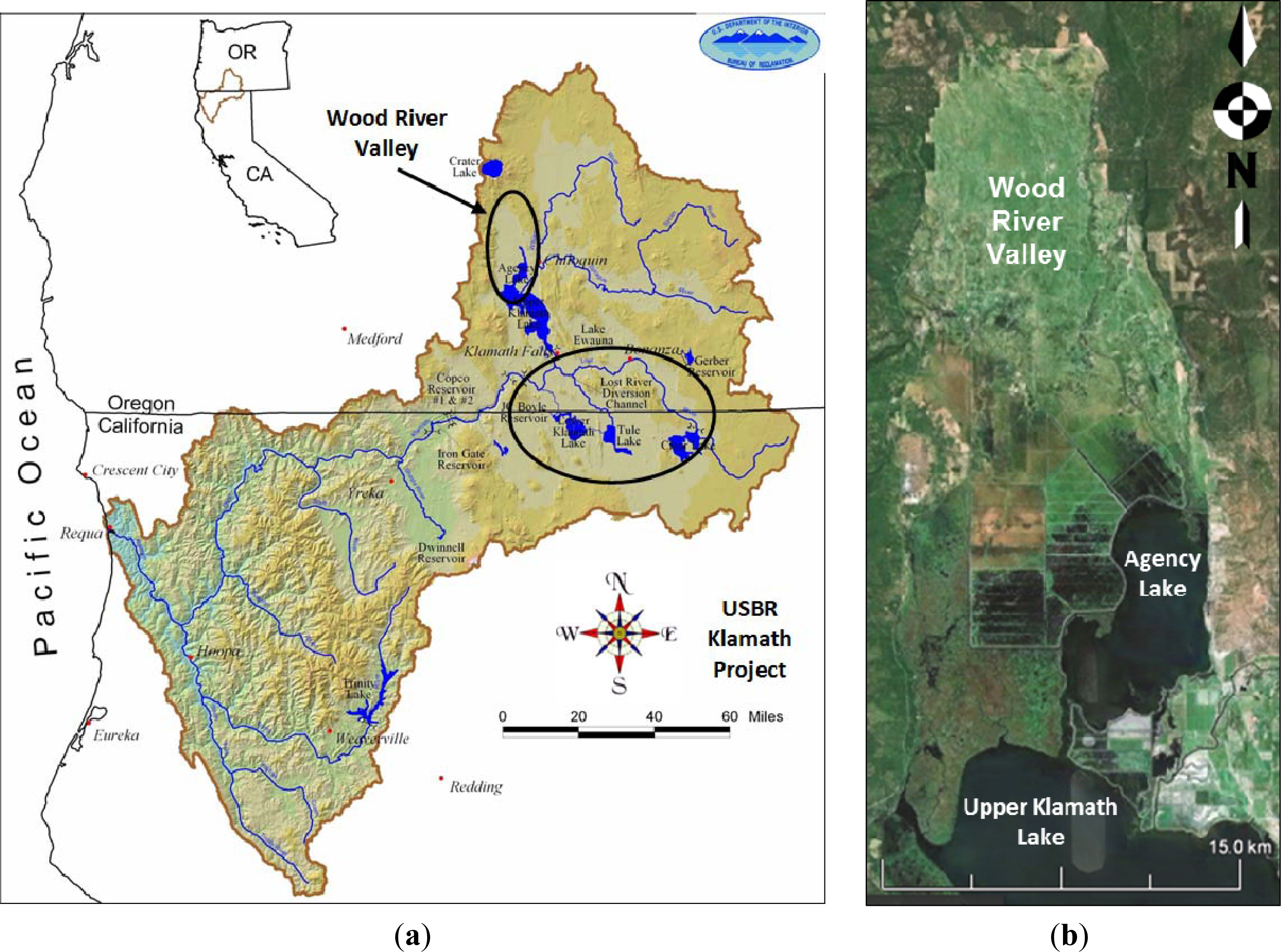
The headwaters of the Klamath Basin in Oregon and northern California are in an agricultural region with extensive irrigation for livestock and crop production. The primary hydrologic feature in the Upper Klamath Basin is 250 km2 Upper Klamath Lake, including connected Agency Lake which drains into the Upper Klamath Lake. The U.S. Bureau of Reclamation (USBR) manages lake levels to support two endangered species of Suckers, releases water to the mainstem Klamath River which supports endangered Coho salmon, and provides irrigation water to thousands of farms and ranches in the Klamath Project (see Figure 1).
The Klamath Project was the first irrigation project undertaken by USBR. It is located below Upper Klamath Lake along the Oregon–California border. Project construction began in 1906 and water was first made available for irrigation in May 1907. The Klamath Project supplies farmers on 91,000 ha (225,000 ac) with irrigation water. The main sources of Klamath Project water are Upper Klamath Lake, the Lost River Basin, and the Klamath River.
Relatively recent protected species listing and fish kills have brought increased pressures on water use in this basin. The Lost River and Shortnose Suckers were listed as endangered species in 1988. In 2001, irrigation water deliveries to the Klamath Project were halted in order to maintain sufficient water levels in Upper Klamath Lake to support the endangered Suckers. During the summer of 2002, drought conditions and low flows in the entire Klamath Basin contributed to high temperatures in the lower reaches of the Klamath River resulting in a massive die-off of salmonids, including endangered Coho, from disease. These pressures resulted in widespread efforts to restore habitat and reduce consumptive water use in the Upper Klamath Basin.
One such effort continues in the Wood River Valley. This valley lies directly north of Upper Klamath Lake, provides 25 percent of the water inflow to Upper Klamath Lake, and is almost exclusively flood-irrigated seasonal cattle pasture. (The valley is managed for grazing only and there are no cuttings made.) Livestock are brought to the valley in April, and are removed in September, October, and November. The Wood River Valley is outside of the USBR Klamath Project area, and generally has sufficient water resources to meet irrigation needs. However, in response to the Klamath Project water shortage in 2001, ranchers in the Wood River Valley formed the Klamath Basin Rangeland Trust (KBRT) to organize irrigation forbearance in the basin. Irrigation forbearance involves the voluntary withdrawal of irrigation water from certain pasture lands in order to leave the water in-stream, increasing inflows to Upper Klamath Lake. Farmers who agreed to be part of this program can only use their water for watering livestock and not for irrigating pasture. Due to the anticipated reduced carrying capacity of the land in terms of head of cattle, farmers in the program were compensated by various government agencies throughout the project, including USBR and the Natural Resource Conservation Service (NRCS).
The objective of this remote sensing study was to evaluate, within the limited confines of the Wood River Valley (see 
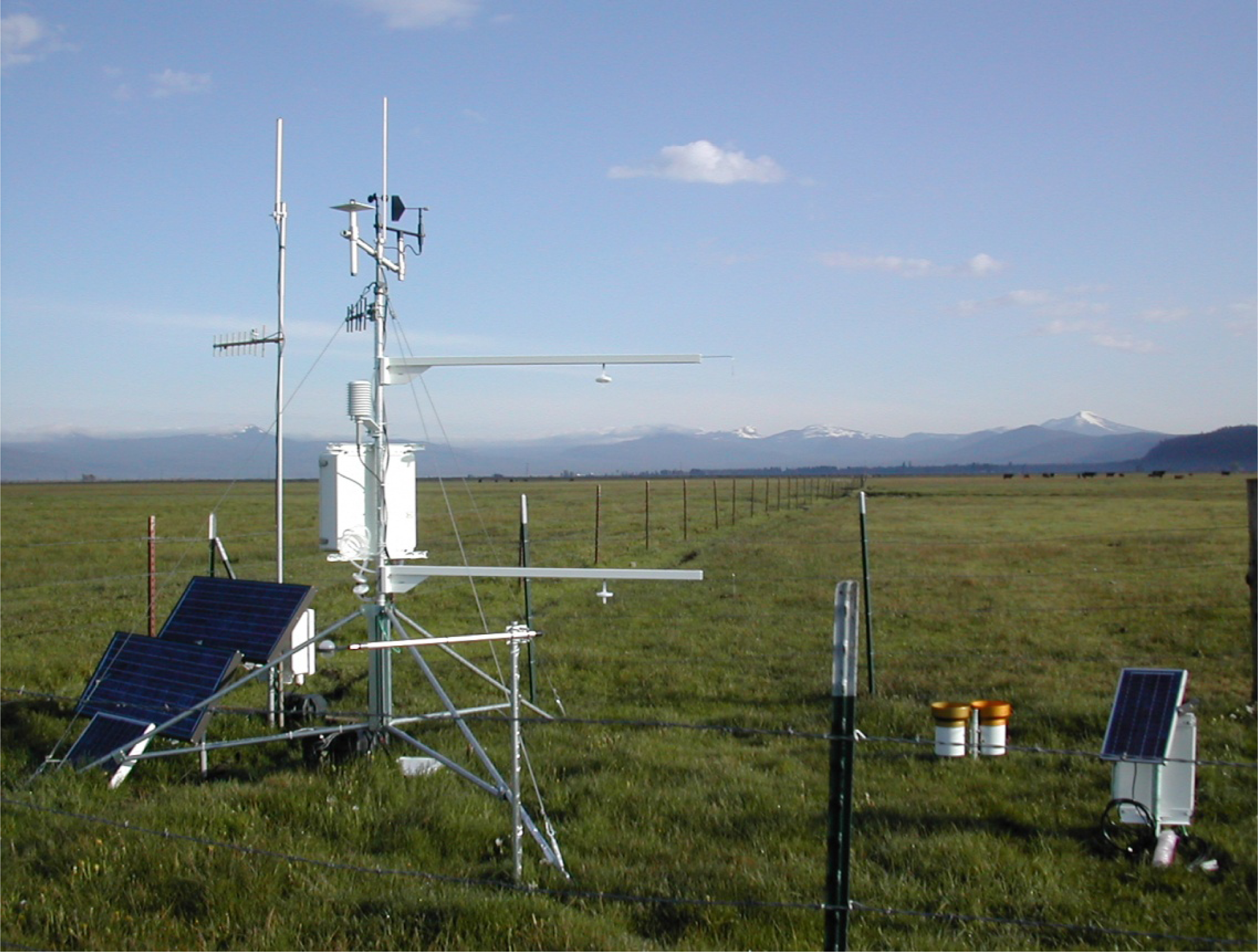
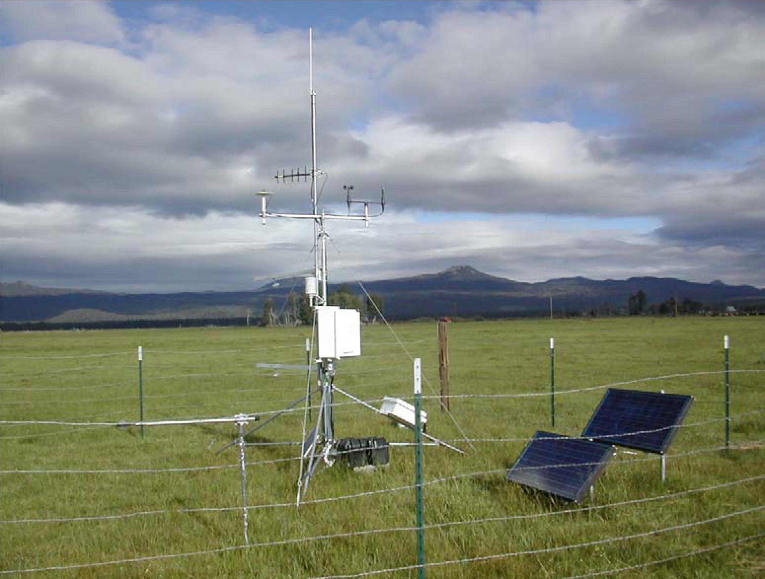
Figure 1), whether or not remote sensing could be used to quantify the water savings from irrigation forbearance in terms of reduced evapotranspiration on a basin-wide scale. This is a real test of the accuracy and resolution of the remote sensing method and platform in that irrigated and unirrigated fields lay virtually one next to the other in this valley. As will be described later, ground-based Bowen ratio stations were available to evaluate actual vegetative canopy water use over specific irrigated and unirrigated sites. However, remotely sensed data would be the only tool available to meet the challenge of evaluating the effects of irrigation forbearance on a valley-wide scale.

1.2. Landsat Earth Observing Satellites

The first satellite in the Landsat program was launched in 1972 and the program recently completed 40 years of continuous monitoring of Earth’s resources. The primary instrumentation on Landsat 1 was the Return Beam Vidicon (RBV) (red, green and infrared bands) at 80-m resolution but this system was identified as the cause of electrical transients which caused instability problems and was switched off. The very much experimental secondary system on Landsat 1 was the 79-m resolution multispectral scanner (MSS) which quickly became the most important sensor package. Variations of the MSS have remained an integral part of the Landsat sensor system. Numerous developments were made to the Landsat sensors both in terms of wavelengths and resolution over the decades. Landsat 3 was the first to have a thermal band as part of the MSS, however the channel failed shortly after launch. Landsat 4 and 5, launched in 1982 and 1984 respectively, continued with the MSS sensor package and added the Thematic Mapper (TM) which included a thermal infrared band. Instrument upgrades produced an improved ground resolution of 30-m and three new bands.
It is the thermal band at the relatively high resolution that enables calculation of components of the energy balance and therefore the evapotranspiration from irrigated fields. Table 1 indicates the MSS and Thematic Mapper (TM) bands incorporated into the Enhanced Thematic Mapper Plus (ETM+) of Landsat 7 used in this study. It should be noted that the Landsat Data Continuity Mission (LDCM) was recently launched (11 February 2013) and put two improved sensor packages, the Operational Land Imager (OLI) and Thermal Infrared Sensor (TIRS), into orbit (see Table 1). The LDCM designation was recently changed to Landsat 8 upon successful insertion into orbit and completion of tests of the sensor systems. This system will replace Landsat 5 which was decommissioned in Jan 2013 (27 years beyond its 3-year design life) and is expected to fill in data gaps caused by the loss of the Landsat 7 scan line corrector (SLC) since 2003.
All previous MSS, TM and ETM+ sensors were “whiskbroom” imaging radiometers that employed oscillating mirrors to scan detector fields of view cross-track to achieve the total instrument field of view. Both the OLI and TIRS use long, linear arrays of detectors aligned across the instrument focal planes to collect imagery in a “push broom” manner. The Landsat 8 push-broom array is expected to significantly improve the signal to noise ratio and reduce component wear. (There are new calibration challenges associated with the push-broom design as discussed in Ungar [1] and Irons [2]). Landsat 8 also has an additional band which will enhance the ability to quantify the effects of atmospheric water vapor on the scene. As indicated in Table 1, Landsat 8 has two thermal bands at 100-m resolution. The two bands will enable atmospheric correction of thermal data using a split-window algorithm (Caselles et al., [3]). Caselles et al. [3] have shown that use of two separate, relatively narrow thermal bands minimizes the error in retrieval of the land surface temperature.

1.3. Applications of Landsat Data

There have been numerous applications of Landsat data for the evaluation of water resource utilization, energy balance analysis and water balance analysis. Some have relied on shortwave vegetation indices (VI) approaches, for example the Red Vegetation Index (RVI) (defined as near infrared reflectance divided by red reflectance), Difference Vegetation Index (defined as near infrared reflectance minus red reflectance), and Normalized Difference Vegetation Index (NDVI) (defined as the near infrared minus the red reflectance divided by the sum of the near infrared plus red reflectance). Such vegetation indices indicate relative plant productivity, density and vigor, and have been successfully used to map crop coefficients over agricultural landscapes (Hunsacker et al. [4]). However, as indicated by Anderson et al. [5]), the relationship between the crop coefficient and the VI must be derived empirically for each crop/vegetation type using local ET measurements. Gonzalez-Dugo et al. [6] compare operational remote sensing methods, including applications of radiometric surface temperature contrasted with vegetation indices, for estimating crop ET. One of their conclusions is that methods based on the VI-basal crop coefficient approach require a coupled soil-water balance model to account for soil evaporation or reduction in transpiration due to stomatal closure under water stress conditions. Melton et al. [7] derive crop coefficients based on NDVI and would similarly need a method to account for stomatal closure under water stress conditions to estimate actual crop ET.
Kalma et al. [8] present a comprehensive review of evaporation estimating methods which use remotely sensed surface temperature data. These methods can basically be divided into the following categories: (a) radiation balance and surface energy balance; (b) regression models using the difference between surface and air temperature; (c) methods which use the time rate of change in surface temperature with atmospheric boundary layer (ABL) models; (d) regression models using surface temperature and meteorological data; and (e) methods which use surface temperature with land surface process models (LSM). It should be noted that categories (b) and (d) which are based on regression analysis tend to be site and crop specific. Categories (c) and (e) require additional sophisticated ABL and LSM models which have their own inherent degree of uncertainty. This article will focus on category (a) which requires development of procedures for determining the radiation and energy balances as described later.
A key concept in application of relatively high resolution Landsat data is the “sharpening” of thermal band data using the higher resolution optical band data. This methodology is based on the procedure developed by Kustas et al. [9], later utilized by Anderson et al. [10], as described in Agam et al. [11]. The assumption is that there is a unique relationship between NDVI and the radiometric surface temperature, Ts. Anderson et al. [5] clearly demonstrate the “sharpened” 30-m field-scale resolution which is attainable using the TIR sensor system on Landsat at 120-m resolution (Landsat 5) or 60-m resolution (Landsat 7) compared to the MODIS thermal band at 1,000-m resolution. (The MODIS thermal band data can also be “sharpened” using this procedure, but only to a minimum of 250-m at nadir.) Anderson et al. [5] show that water use by riparian vegetation can be resolved using Landsat data whereas the water course is not even visible at the resolution of MODIS scenes.

2. Method of Ground-Based Data Analysis

2.1. Theory and Instrumentation

Two Bowen ratio stations were deployed in the Wood River Valley to estimate the difference in transfer of moisture to the atmosphere from soil and vegetation (evapotranspiration) between an irrigated and unirrigated pasture site. The Bowen ratio system used the 023/CO2 Bowen Ratio System designed by Campbell Scientific, Inc. (CSI) that incorporates the LI-COR LI-6262 high-speed (10-Hz) infrared gas analyzer (IRGA) for water vapor gradient, fine-wire thermocouples for the air temperature gradient, REBS Q*7 net radiometer and two Hukseflux self-calibrating soil heat flux plates buried at 8-cm depth with two thermocouples at 2-cm and 6-cm depths to integrate heating effects to the soil surface. The energy balance was computed every 20-min. KL03 at the unirrigated site (Thomas Ranch) came on-line on 10 April 2004 (DOY 101) and the second station, KL04 at the irrigated site (Owens Ranch), was not fully operational until 23 April (DOY 114). Both sites were chosen for their excellent fetch conditions and uniform vegetation, i.e., on the order of 1000-m in the direction of predominant wind (see Figures 2 and 3). The Bowen ratio stations also include a precipitation gauge and meteorological and near-surface soil moisture data for application of the Penman-Monteith evapotranspiration estimating method. Additionally, both Bowen ratio sites had soil moisture profile measurements.
The Bowen ratio is defined as the ratio of sensible to latent heat flux,
β = H L E
where
  • β = Bowen ratio (dimensionless);
  • H = sensible heat flux (W/m2);
  • LE = latent heat flux (W/m2).
The governing surface energy balance equation given as,
R n = G + L E + H
where
  • Rn = net radiation (W/m2);
  • G = soil heat flux (W/m2).
Equation (2) can be rearranged in terms of the Bowen ratio as,
L E = R n G 1 + β
The evapotranspiration (ET) as an equivalent depth is equal to LE/λ where λ is the latent heat of vaporization. Assuming one-dimensional vertical transport of a scalar quantity above the surface, and the eddy diffusivity of water vapor equal to the eddy diffusivity of heat, the Bowen ratio can be calculated from measurements of temperature and vapor pressure gradients as,
β = γ Δ T Δ e
where
  • ΔT = air temperature gradient (°C);
  • Δe = vapor pressure gradient (kPa);
  • γ = psychrometric constant (kPa/°C).
The Ohmura [12] data quality control and data screening algorithms were implemented for analysis of data from the Bowen ratio stations. The basic concept is that the Bowen ratio method is based on certain theoretical considerations. There are some combinations of components of the energy balance coupled with sensor sensitivity that violate the assumptions of the Bowen ratio theory. One of these is the flux-gradient relationship which specifies that fluxes must always go “down gradient”, i.e., in the direction from higher to lower potential. Other combinations cause the Bowen ratio itself to be close to −1, at which time the denominator in Equation (3) goes to zero and the latent heat flux, LE, goes to infinity. The Ohmura data quality control procedure screens out the data which violate the flux-gradient relationship as well as cases when the Bowen ratio is close to −1. The data screening at each time step depends on the magnitude of the components of the energy balance and the sensitivity of the instrumentation, specifically the fine-wire thermocouples used for air temperature measurement and the IRGA used to measure water vapor gradients.

2.2. Example Results from the Bowen Ratio—Energy Balance System

The following results are presented to demonstrate the robustness of the energy balance data as measured by the Bowen ratio systems and to indicate that a difference in the measured latent heat flux represents a real difference in the vegetative evapotranspiration (ET). The cumulative latent heat flux (expressed as the equivalent depth of evapotranspiration, ET) was calculated to compare results from the two stations. Figure 4 indicates these results for a 20-day period (DOY 130 to 150) in May early in the growing season when field conditions everywhere in the basin produce a soil moisture content between saturation and field capacity. At this stage of the growing season there is no reason to expect a difference in evaporative fluxes between the two stations. (The two traces in the figure are slightly offset because the two stations came on-line on different dates.) An almost mirror-image response of the two sensor systems, located over 11 km apart, during the hours of each 24-h cycle can be observed. Although the fluxes are not quite identical over this period, there is less than 1 percent difference between the two sites. Such well-behaved responses in field experiments are rarely achieved and give us confidence that when there are differences between the two sites as the unirrigated site dries down, these differences will be real.
Figure 5a,b indicates the diurnal energy balance for DOY 288 (14 October) at KL03 and KL04, respectively. The first contrast between these two plots is the net radiation which is noticeably higher at KL04 than KL03. This is due to the fact that the unirrigated (KL03) field is much more yellow at this time of the season than the greener, irrigated (KL04) site, causing increased reflectance (i.e., albedo) for shortwave radiation at KL03. This decrease in net shortwave radiation leads to an overall decrease in net radiation at the unirrigated (KL03) site.
The partitioning of net radiation is very different at the two sites. The sensible heat flux (H) is much greater in magnitude than the latent heat flux (LE) at KL03. These conditions are reversed at KL04. The vegetation at the irrigated site is able to transpire at a much higher rate than that at the unirrigated site. The soil heat flux at KL03 is also much lower (∼45 W/m2 peak) than typical fluxes at KL04 (∼100 W/m2 peak), in spite of increased vegetation shading at the irrigated site. The soil heat flux at KL04 is higher due to the much higher thermal conductivity of wet soils as contrasted to dry soils.
Figure 6 indicates the comparison of the cumulative evapotranspiration for the two sites from the start of the season (DOY 122—01 May) until the end of the irrigation season (DOY 274—30 September). Both sites start with relatively high levels of soil moisture, as well as a high water table, due to significant over-winter precipitation including melting of a relatively deep (on the order of 1-m) snowpack. It can be observed that for the first almost 50 days there is very little difference in the cumulative evapotranspiration between the sites. As shown in Figure 4, during the 20-day period from DOY 130 to 150 there is virtually no difference in cumulative evapotranspiration between the two sites. After about DOY 180 (i.e., end of June) the two sites are on distinctively different paths, with the evaporative flux rate from KL04 (irrigated) significantly higher than that from KL03 (unirrigated). This divergence continues until the end of the irrigation season when there is a measured difference of 248 mm in evapotranspiration between the two sites. This is equivalent to an unbiased difference (dividing by the average cumulative ET of the two sites) of 40 percent between the two sites.

3. Method of Landsat Data Analysis

One of the key challenges of this project was how to interpret the point data of the Bowen ratio stations within the context of valley-wide crop water use. It was decided to apply Landsat image data analysis to quantify the distribution of actual evapotranspiration over the valley, as indicated in Section 1.2, the ability to quantify the effects of irrigation and plant water use down to a 30-m resolution is a very positive attribute of using Landsat thermal band data. Given the scale of the unirrigated fields in the Wood River Valley, i.e., those that came under the voluntary forbearance program, the only possibility to retrieve the contrast in ET between irrigated and unirrigated fields was to use relatively high resolution Landsat data.

3.1. Image Selection

The time period of interest was the 2004 irrigation season, from April through September. After review of available imagery for the Wood River Valley on the U.S. Geological Survey (USGS) Global Visualization web page ( 
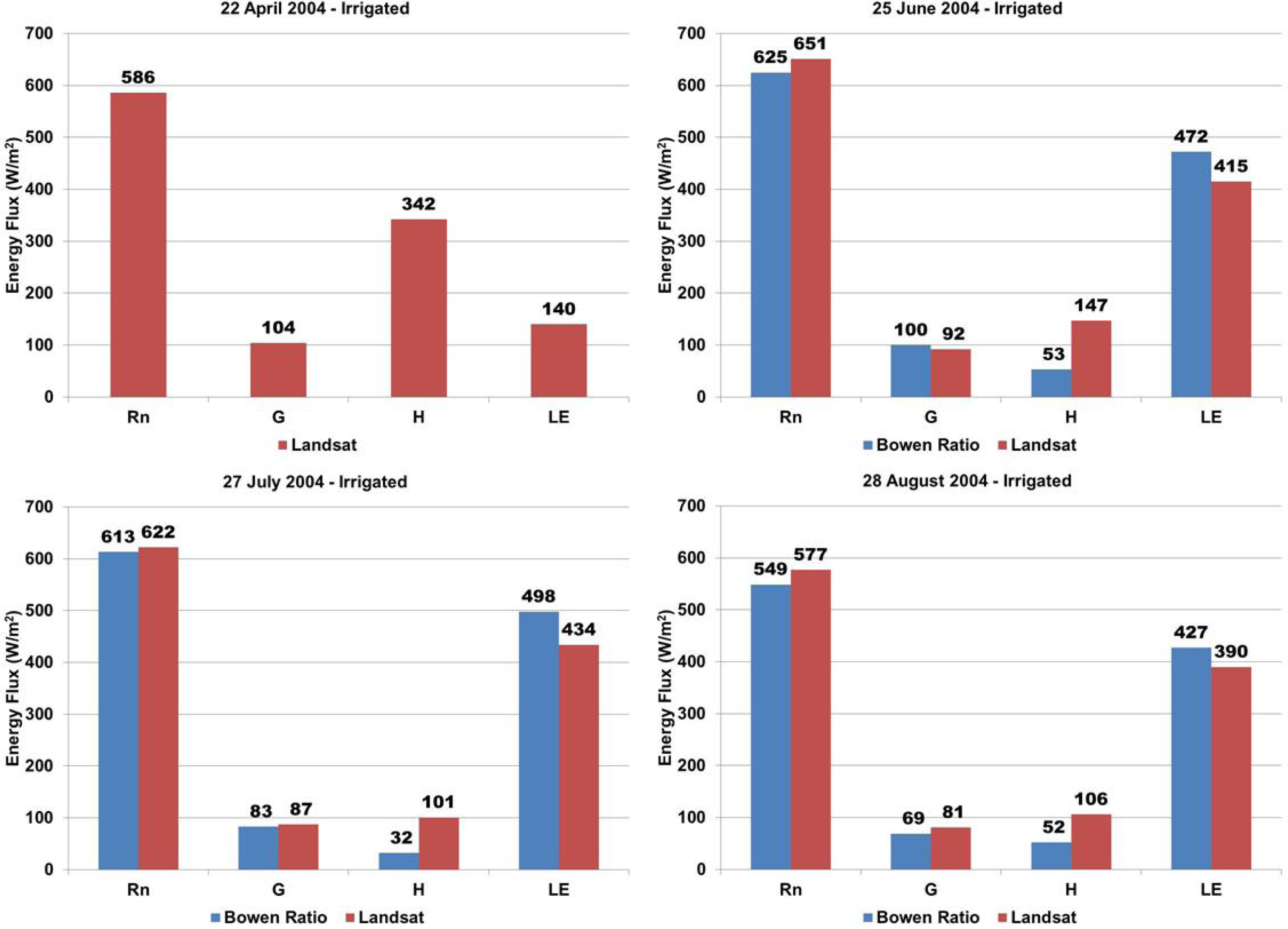
http://glovis.usgs.gov/), four Landsat 7 scenes were selected for the 2004 growing season. The dates selected were 22 April (DOY 113), 25 June (DOY 177), 27 July (DOY 209) and 28 August (DOY272). [Landsat Worldwide Reference System (WRS) Path 45, Row 30, cloud cover equal to or less than 2 percent and image quality equal to 9 for all four scenes.] These dates cover most of the range of conditions found during the irrigation season.
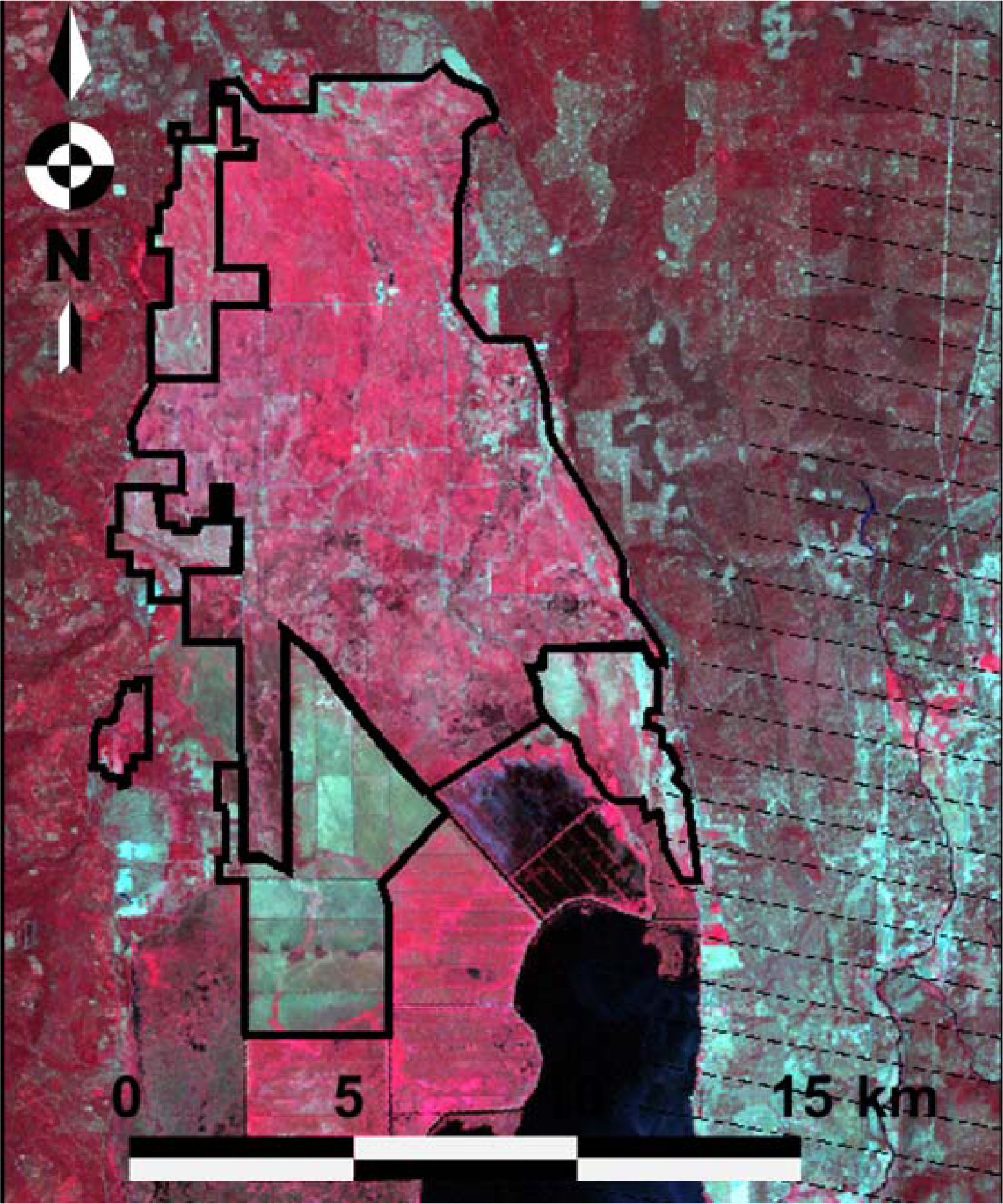
The selected images were obtained from the USGS/EROS Data Center and initial image processing and georectification was performed by Watershed Sciences, Inc. of Corvallis, Oregon. This step is no longer required as Landsat scenes available on the USGS website are now georectified. Landsat 7 bands 1 through 5 and 7 had a pixel resolution of 28.5 m. The pixel resolution of band 6, originally 57 m, was re-sampled to 28.5 m so that the entire scene was at the same resolution. Almost the entire area of interest was near the center of the images, so the scan lines from the disabled SLC had a negligible impact (Figure 7).
It should be noted that there are additional Landsat 5 scenes available for the study period. At the time the analysis was completed, the recommendation was to use Landsat 7 instead of Landsat 5 as there was concern regarding potential Landsat 5 sensor degradation. This concern is no longer valid since modern radiance calibration has transformed Landsat 5 images into high accuracy retrievals. However, as the study area was very minimally affected by the SLC-off scan lines, the decision at the time the data were analyzed was to use only Landsat 7 images. Including additional Landsat 5 images with current calibration methods would improve the analysis but would require a significantly expanded study. As will be demonstrated, comparing the Landsat 7 results to the Bowen ratio findings shows that the limited number of scenes used were sufficient to develop the crop coefficient curve over the season.

3.2. Calculation of Instantaneous ET Flux from Landsat Data

Price [13] developed the concept of using information from within the satellite image to scale between TIR end-member pixels representing non-limiting moisture availability and limited extractable moisture. Kustas and Norman [14] presented an overview of the most common remote sensing algorithms to estimate heat and evaporation fluxes up to that time. Bastiaanssen et al. [15] and Bastiaanssen [16] developed the Surface Energy Balance Algorithm for Land (SEBAL) to calculate the energy partitioning at a regional scale with minimum ground data. Later work was incorporated into the Mapping Evapotranspiration with Internalized Calibration (METRIC) program (Allen et al. [17]).
The approach used to calculate instantaneous, daily and seasonal ET across the Wood River Valley using Landsat data precisely followed the 2002 METRIC Advanced Training and Users Manual with ERDAS IMAGINE software (Allen et al. [18]). These processes are therefore described in the Manual. There are, however, several steps in the process where the user is required to make critical decisions related to the application of the algorithm under site specific conditions. Those steps and the approach taken by the user are described below.

3.2.1. Soil Adjusted Vegetation Index (SAVI) Constant (L)

SAVI is used to calculate Leaf Area Index, necessary to determine surface and broadband emissivities. SAVI is calculated using,
S A V I = ( 1 + L ) ( ρ 4 ρ 3 ) ( L + ρ 4 + ρ 3 )
where
  • ρ3, ρ4 = band 3 and 4 reflectance;
  • L = SAVI constant dependent on soil characteristics.
The value of L depends on the soil characteristics of the area during the time frame of interest. The resulting Leaf Area Index (LAI) is the main factor that regulates an appropriate L value. An expected LAI for heavily grazed pasture (ryegrass) is 1, while lightly grazed pasture (ryegrass) would be 3. LAI in the Wood River Valley ranges between these values, but is often less than 3, especially at the unirrigated sites.
The June, July, and August images were used in the L value analysis. SAVI was calculated using an L of 0.1, 0.2, 0.3, 0.4, and 0.5. L = 0.1 resulted in the most constant SAVI values on irrigated ground, while L = 0.5 appeared to be the best fit on irrigated ground. LAI was computed using the SAVI values with L = 0.1 and L = 0.5. Using L = 0.1 resulted in LAI values from just under 1 to 6. That much variation in the LAI on the grazed pastures is not expected, and it is doubtful that LAI reaches 6. However, when using L = 0.5, the range of LAI values dropped drastically, ranging from less than 0.5 to just under 2. These values are lower than would be expected. LAI was then calculated using a SAVI from L = 0.3, which resulted in LAI between 1 and 3. These are more realistic values for the area of interest. Therefore, 0.3 was chosen as the L constant value.

3.2.2. Corrected Thermal Radiance in Surface Temperature

The surface temperature can be calculated from Landsat data using the narrow band emissivity and the corrected thermal radiance (Rc). Corrected thermal radiance is computed by the following equation from Wukelic et al. [19],
R c = L 6 R p τ n b ( 1 ɛ n b ) R s k y
where
  • Rc = corrected thermal radiance (W/m2/sr/μm);
  • L6 = spectral radiance for band 6 (W/m2/sr/μm);
  • Rp = path radiance for band 6 (W/m2/sr/μm);
  • τnb = narrow band transmissivity of air (W/m2/sr/μm);
  • εnb = narrow band emissivity (-);
  • Rsky = narrow band downward thermal radiation from a clear sky (W/m2/sr/μm).
Values for Rp and τnb can be found from radiosonde profiles from the area of interest near the time of the image. If these data are not available, the value of Rp can be set to 0 and τnb can be set to 1. Rsky can be calculated from ground data, but could bias the correction without real values for the other terms as well. As there were no radiosonde data available for the Wood River Valley, the values used were Rp = 0, τnb = 1, and Rsky = 0.

3.2.3. Selection of the “Hot” and “Cold” Pixels

The METRICTM approach scales sensible heat (H) values across an image based on the surface temperature. It uses a Calibration using Inverse Modeling at Extreme Conditions (CIMEC) method for estimating sensible heat flux. CIMEC is based on inverse modeling of the near surface temperature gradient (dT) for each image pixel based on a relationship between the dT and radiometric surface temperature at two “anchor” pixels (Kjaersgaard et al. [20]). The anchor pixels set the boundaries of the sensible heat flux in the energy balance. One pixel is representative of a well-watered and fully-vegetated area with maximum ET (“cold” pixel) and the other is representative of a dry, poorly vegetated area where ET is assumed to be zero (“hot” pixel).
Use of the CIMEC method avoids the need to use the absolute surface temperature and therefore minimizes the influence of atmospheric corrections and uncertainties in surface emissivity. This avoids the problem of inferring the aerodynamic temperature, the temperature which provides an estimate of the sensible heat flux (Norman and Becker [21]), from the radiometric surface temperature and avoids the need for near-surface air temperature measurements. The method estimates the difference between two near-surface air temperatures assigned to two arbitrary levels and does not require the air temperature at any given height (Irmak et al. [22]; Allen et al. [23]).
Guidelines to follow for the cold pixel include an LAI between 4 and 6 and surface albedo between 0.18 and 0.24. However, since the area of interest is short grass cover instead of crops, the LAI generally ranges between 0.3 and 2.5, increasing with growth over the season. It was therefore necessary to look for LAI values around 1 in the early season, and 1.5 to 2 later in the season. Guidelines to follow for the hot pixel include an LAI of 0 to 0.4 (little or no vegetation) and a surface albedo similar to other bare, dry areas in the image representative of bare soil conditions.
The surface temperature images were used to determine the existing range of temperatures and identify potential areas for the anchor pixels. Then the LAI and albedo images were used to select pixels that fell within appropriate ranges. It is important to note that the authors have an intimate knowledge of the valley floor, and were able to identify appropriate and representative areas and then use the images to select the most appropriate pixels. Multiple appropriate pixels were selected and the authors’ knowledge of ground conditions was used to make the best choice. The process was repeated for each month.
The cold pixel was chosen in a fully irrigated, fully vegetated pasture. ET at the cold pixel was calculated as 1.05 (ETr) (for reference ET based on alfalfa) for all months. The hot pixel was chosen from within an area with no vegetation. As there were no precipitation events near the date of the images, and visual inspection confirmed very dry conditions, the assumption that ET = 0 is valid for the June, July, and August images. While there was no precipitation leading up to the date of the April image, visual inspection of the site suggested that there was still residual soil moisture from winter snowmelt. As the information needed to develop a soil water balance since the end of the snowmelt was not available, ET at the hot pixel at the time of the April image was estimated as 0.25 (ETr) based on moderate soil moisture conditions at the time (where ETr is based on alfalfa). This value was used in H calculations for the April image.

3.2.4. Soil Heat Flux (G)

The data set collected for this project gives us an advantage in the various calculation steps since we can verify the results compared with ground-based data, at least for two locations representative of unirrigated and irrigated conditions, KL03 and KL04, respectively. The ratio of soil heat flux to net radiation, G/Rn, was originally given by the following equation based on NDVI values developed by Bastiaanssen [15] for values near midday,
G R n = T s α ( 0.0038 α + 0.0074 α 2 ) ( 1 0.98 N D V I 4 )
where Ts is the surface temperature (°C), α is the surface albedo, and NDVI is the Normalized Difference Vegetation Index, computed using Landsat bands 3 and 4. Alternatively the procedure of Tasumi [24] takes vegetative cover explicitly into account through the leaf area index (LAI) and is given as,
G R n = 0.05 + 0.18 exp ( 0.521 L A I ) for L A I > 0.5
G R n = 1.80 ( T s 273 ) R n + 0.084 for L A I < 0.5 ( ~ bare soil )
Applications of METRIC in southern Idaho have shown that both methods provide relatively accurate values of G. Both methods were tested for the southern Oregon site. A model for each method was built in ERDAS IMAGINE Model Maker platform and the output compared to the G measured at the Bowen ratio stations. The June image at the irrigated site resulted in over 100 percent error using both methods; excluding June the error ranged from 36 to 89 percent using the NDVI method and 6 to 87 percent using the LAI method. Personal communication with M. Tasumi revealed that when looking at areas that have relatively homogenous agricultural cover (such as the Wood River Valley) the LAI derived G is generally preferred. NDVI is considered applicable for areas with variation in land use or crops, where there would be more variable LAI. The LAI method for calculating G/Rn (Equations (8) and (9)) was chosen for this project. The soil heat flux is calculated by multiplying the above ratio by the net radiation output of the radiation models. However, the magnitude of the errors indicated point out the potential for improvement in determination of the soil heat flux. These errors are no doubt affected by the thermal conductivity of the soil which is radically different for wet versus dry soil conditions.

3.2.5. Reference ET

Reference ET was calculated with meteorological data from KL03 and KL04 using the REF-ET software package (Allen [25]). Reference ET using the FAO 56 Penman-Monteith method was calculated for 20-min time steps over the full season, as this was the recording interval of the Bowen ratio stations. While there were additional ground data available from the Bowen ratio stations that could be input into REF-ET, the decision was made to limit weather data to the inputs used in the 2002 manual (Allen et al. [18]) to be able to compare to typical results.

3.3. Calculation of Seasonal Evapotranspiration and Extrapolation across Valley

Once instantaneous ET is known, it can be translated into daily ET by assuming that the ratio of actual to reference ET, also termed the reference ET fraction, at the time of satellite overpass remains constant for the day (Irmak et al. [22] and Allen et al. [23]). Seasonal ET can then be derived from the daily ET. This process essentially assumes that ET for the area of interest changes in proportion to the change in reference ET and, more importantly, that the crop coefficient (ratio of actual ET to reference ET) remains constant or changes in a linear or some other well-defined manner until the time of the next satellite overpass (Allen et al. [17]).
This project determined total ET for the time period of 01 May to 30 September. The available Landsat images were used to represent to following time periods: 25 June image for the period 01 May–15 July; 27 July image for the period 16 July–15 August; 28 August image for the period 16 August–30 September. For each time period a reference ET fraction, ETrF, was calculated at the time of satellite overpass based on an alfalfa reference and this value was assumed to hold constant until the next time period. This is equivalent to using a step-wise linear crop coefficient over the growing season. Daily reference ET was calculated for each time period and multiplied by ETrF to get the actual ET. All daily ET values were summed to get the seasonal ET.
Allen et al. [23] and Irmak et al. [22] caution that cloud cover, irrigation timing, and a reference ET that is not representative of the entire area may complicate accurate calculation of seasonal ET. Cloud cover and irrigation patterns were not an issue in this project, but reference ET bears special consideration. It was determined that one value of reference ET was representative for the entire area of interest. When one observes the incoming solar radiation, air temperature and air relative humidity data, it is not possible to tell without prior knowledge whether the data were taken over the irrigated or unirrigated site. This is due to the effects of turbulent atmospheric mixing in the relatively limited area of the Wood River Valley. While starting in early July, soil water becomes limited at the unirrigated site (KL03) and actual ET begins falling well below reference ET, the reference ET value (representing a well-watered crop and calculated using the FAO 56 Penman-Monteith method) is still uniform throughout the valley.
Subsets of the irrigated areas, and separately non-irrigated areas, were made from the final seasonal ET image. A small portion of the non-irrigated subset was impacted by the Landsat 7 SLC-off scan lines. These data gaps were filled using the ERDAS Imagine nearest neighbor correction process. Statistical tools in ERDAS Imagine were used to determine the average seasonal ET for the irrigated and unirrigated sites.

4. Results and Discussion

4.1. Comparison of Energy Balance Components from Landsat and Bowen Ratio

The results of the energy balance components by application of the reconstructed LE algorithms compared to ground-based measurements for the four Landsat scenes at the irrigated and unirrigated sites are plotted as bar graphs in Figures 8 and 9. It should be noted that the April Landsat scene was at a time of nearly saturated conditions throughout the basin and the presence of some standing water due to melting of a 1-m deep snowpack. The most immediately notable result of the comparison is the close agreement in the net radiation component of the energy balance for both the irrigated and unirrigated sites. This component is always the largest of the energy balance, so getting good agreement between these values is important. The soil heat flux component is generally the smallest of the energy balance components so while there are times with significant differences between measured and computed values (e.g., June at the unirrigated site), this tends to not have a significant impact on the computed latent heat flux. Differences between measured and computed sensible heat flux can also be significant, e.g., July at the unirrigated site and June at the irrigated site. (April also has a problem at the irrigated site but the nearly saturated soil profile conditions play a role in this error. These wet conditions mean that the range of surface temperatures between the “hot” and “cold” pixels needed for the iterative scheme to compute the sensible heat flux is very limited. The internal calibration achieved by using the full range of surface temperature between the hot and cold pixel is therefore weakened.) However, the relative magnitude of the sensible heat flux is such that the latent heat flux results tend to have less of an error. Assuming that the Bowen ratio station data represent the “ground truth” for the sake of argument, the absolute value of the error (or difference in any case) in the latent heat flux varies from a minimum of 9 percent (August at irrigated site) to a maximum of 30 percent (July at unirrigated site). The average absolute value of the latent heat flux error for the irrigated site is 11 percent for the three scenes (i.e., excluding April for which an insufficient number of sensors were operational on this date) while the average error is 22 percent at the unirrigated site for all four scenes. These differences are felt to represent errors of the LE estimate due to the robustness of the Bowen ratio station results demonstrated in Figures 4 and 6.
These results are similar in magnitude for instantaneous differences as those reported elsewhere. Kalma et al. [8], in comparing some 30 validations of various remote sensing methods applied to evaporative flux measurements, indicated difference on the order of 15 to 30 percent. Morton et al. [26] in comparing five Bowen ratio sites and four eddy covariance sites with Landsat derived ET over agricultural sites in Nevada reported daily mean absolute differences on the order of 1 to 27 percent with the mean for all sites on the order of 11 percent. Morton et al. [26] indicated that the Bowen ratio and eddy covariance daily ET measurements were assumed by Maurer et al. [27] to be accurate to within 12 percent of actual ET based on the literature and direct comparison at one site. Kalma et al. [8] indicated a possible error for actual ET measurements in the range of 10 to 15 percent, and Wilson et al. [28] indicated a mean energy balance closure error on the order of 20 percent for 22 FLUXNET sites over 50 site-years using eddy covariance instrumentation. A systematic underestimation of the latent and sensible heat fluxes was the source of the closure errors reported out by Wilson et al. [28].

4.2. Spatial Integration of ET across the Valley to Compare Irrigated and Unirrigated Land

The Landsat data were used to evaluate the spatial integration of evapotranspiration over the Wood River Valley lands within the irrigation exclusion zone (i.e., KBRT project lands) in contrast to the irrigated lands. The results in terms of millimeters per day of evapotranspiration for the four Landsat scenes are shown in Figure 10. Except for the results in April that are suspect due to near-saturated soil profile conditions, the basin wide ET for the irrigated lands is always larger than that for the unirrigated lands, as expected. This difference is seen to increase later in the irrigation season as the unirrigated lands become quite dry. Figure 11 shows the spatial distribution of the latent heat flux over the Wood River Valley using Landsat data for all four scenes with the unirrigated KBRT project lands outlined. Clearly most areas included in the KBRT project lands show significantly lower latent heat flux than the surrounding irrigated lands and this signal is clearer later in the growing season. Without the Landsat TIR resolution the reduced latent heat fluxes from the relatively small fields would not be observable.
As shown in Figure 6 and Table 2, the cumulative ET for the growing season measured at the Bowen ratio stations was 498 mm at the unirrigated site and 746 mm at the irrigated site. The results from the Landsat energy balance approach using the 9 pixels including and surrounding the Bowen ratio station (i.e., 90-m by 90-m), interpolated through the growing season as described, are 511 mm at the unirrigated site and 763 mm at the irrigated site. Assuming the Bowen ratio results are “ground-truth” for the sake of discussion, the differences between these “point” measurements and estimates (in fact trying to account for the footprint of the Bowen ratio station) are 2.6 percent for the unirrigated site and 2.3 percent for the irrigated site, in both cases the Landsat derived values being higher.
The valley-wide seasonal LE images were categorized into irrigated and unirrigated areas to estimate seasonal water savings resulting from irrigation forbearance. The irrigated acreage totaled approximately 10,440 ha and unirrigated area was approximately 4,674 ha. The difference between the mean seasonal ET within each area was used to calculate water savings. As indicated in Table 2, the mean seasonal ET on irrigated ground was 739 mm and mean seasonal ET on unirrigated ground was 566 mm, giving a seasonal reduction of 173 mm of ET due to irrigation forbearance. It is notable that the areal integrated mean ET from Landsat on irrigated land is just slightly lower than that measured at the irrigated Bowen ratio site, and the areal integrated mean Landsat ET for unirrigated land is higher than on the unirrigated Bowen ratio site (Table 2). When the valley-wide values are converted to a volume of water conserved over the growing season, this results in a savings of 805.1 ha·m (8,051,000 m3).
Based on comparisons of ET values derived from Landsat and the Bowen ratio method, these results appear to be quite robust. The Landsat areal integrated results suggest a much lower water savings, 805.1 ha·m, than anticipated by land managers using the “point” data from the Bowen ratio stations (1,154.2 ha·m). The Landsat images reveal more extensive sub-irrigation from neighboring fields and waterways than originally anticipated. This supports findings from a MIKE SHE (hydrology)/MIKE 11 (hydraulics) simulation modeling exercise to determine hydrologic responses to irrigation management in the Wood River Valley (Owens [29]). Owens [29] determined that unirrigated tracts had higher than expected consumptive use because water from the surrounding irrigated tracts was able to flow in the shallow aquifer due to the hydraulic gradient between irrigated and unirrigated lands and provide sub-irrigation. The spatial distribution of sub-irrigation visualized through Landsat analysis will inform managers on how to better direct water savings efforts and ascertain real water savings.

4.3. Potential Discrepancies between Landsat Results and Observed Ground Conditions

However, discrepancies between on-the-ground observations of pasture conditions and Landsat results suggest some caution when interpreting the results. There are several unirrigated areas that demonstrate higher ET from Landsat than expected, including the unirrigated property in the northwest of the valley (Figure 12). Knowledge of these unirrigated pastures leads the authors to question the levels of ET estimated using Landsat on the July and August images. The grass in these pastures was observed to be near wilting and have very limited growth in mid to late summer. Shallow groundwater levels measured by piezometer on the NW property and at KL03 tracked each other fairly closely and were far below initial water table levels close to the surface at the start of the growing season (Figure 12). Nonetheless, there is significant difference in the LE rates reported from pixels around the northwestern well and KL03 in both the July and August images (Table 3). The reason the Landsat analysis resulted in substantial LE rates from the apparently wilted field is not understood. The two sites have the same soil series and the same mixed pasture vegetation dominated by bluegrasses, ryegrasses, sedge and rush communities. The KL03 property was in its third year of non-irrigation, while 2004 was the first year of non-irrigation for the NW property. This may have led to a difference in management and plant cover and/or species distribution. The NW property was likely minimally grazed out of concern for the amount of forage that would be available, and would have a higher percentage of the wet plant species and a shallower rooting depth. Further study is needed to determine if the discrepancies are due to an actual unexpected difference in ET or differences in conditions, e.g., plant species succession as drought is imposed, that were not accounted for. These results may signify a need to more closely account for what may be considered minor differences in ground conditions when applying the Landsat algorithm.

5. Conclusions and Future Applications

It should be noted that the results reported here were derived from a relatively early version of the METRIC algorithm based on the User’s Manual available at the time of analysis (Allen et al. 2002 [18]). Currently, other variations of the algorithm are possible even with the higher resolution, i.e., sharpened, TIR data from Landsat 5 and 7 (Anderson et al. [5]). More recently, Kjaersgaard et al. [20] have demonstrated improved methods for estimating crop ET using METRIC by taking into account antecedent precipitation events through a soil-water balance procedure that adjusts for soil evaporation. Allen et al. [30] indicate an automated procedure for calibration of Landsat data using the METRIC algorithm selecting initial calibration pixels based on NDVI and surface temperature thresholds. Morton et al. [26] describe an automated procedure using a statistical approach based on ETrF distributions and show application to Bowen ratio and eddy covariance stations in Nevada. Such automated techniques will improve data processing efficiency which has been a constraint to application of Landsat data.
This study was undertaken to test the feasibility of evaluating evapotranspiration from irrigated and unirrigated fields of limited extent and in close proximity, i.e., we were not dealing with a homogeneous distribution of irrigated or unirrigated vegetation cover. The Landsat data were the only thermal band data applicable at a scale that was close to the scale of the irrigated and unirrigated fields. Although point measurements for crop water use for the irrigated and unirrigated conditions were available at the Bowen ratio stations, those data did not allow for the evaluation of the effects of differential water application over the Wood River Valley. This was an essential element to judge the utility of the irrigation forbearance program in terms of leaving water in the Klamath River system.
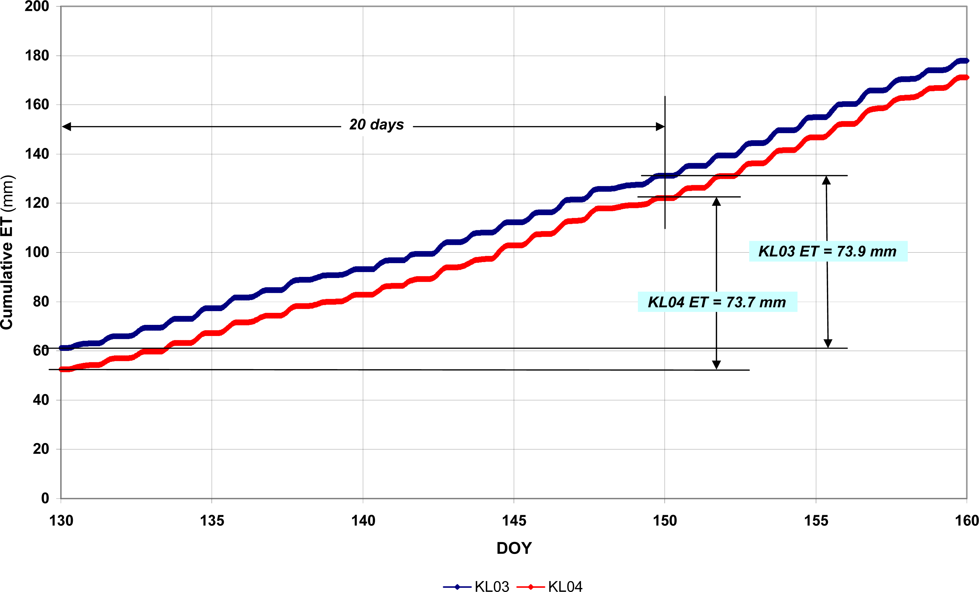
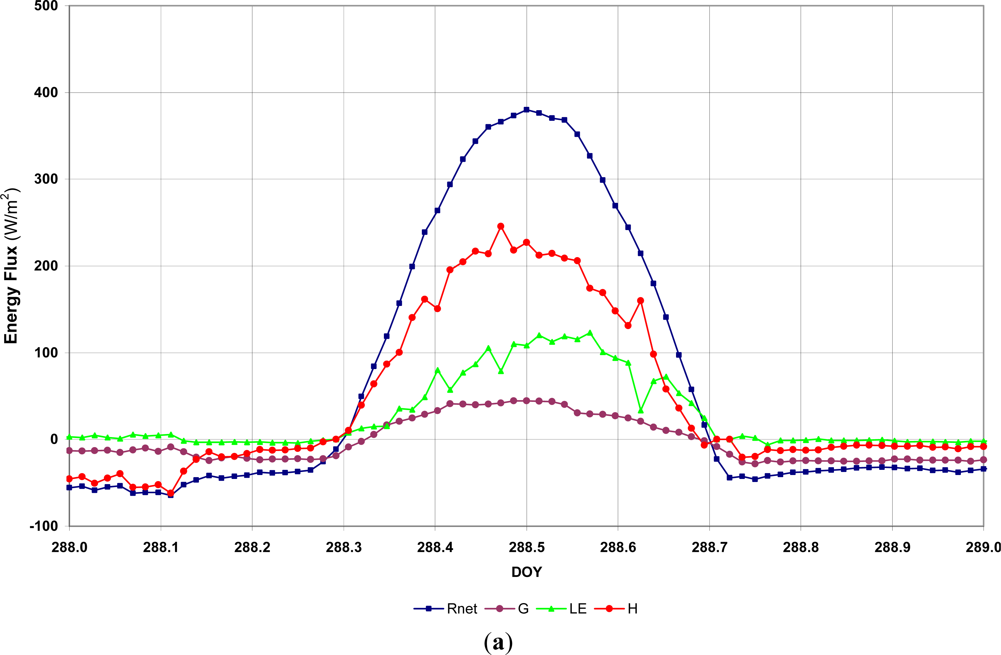
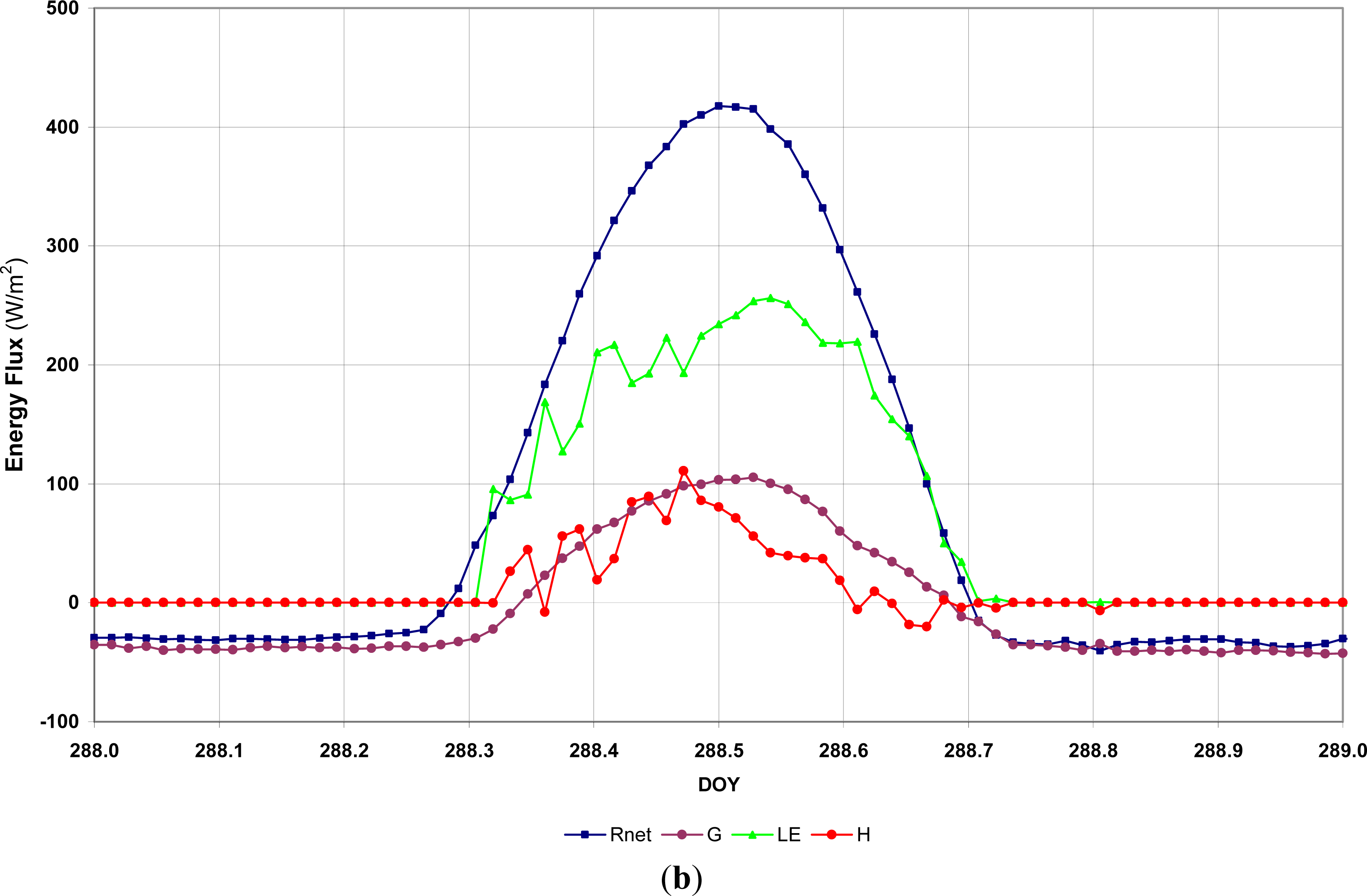
This project demonstrates the utility of discerning the latent heat flux signal from irrigated and unirrigated lands in the same basin using the higher resolution Landsat TIR data. The results of this study indicate difficulty to resolve the latent heat flux with less than approximately 10 percent error over irrigated fields and on the order of double that magnitude for unirrigated fields. This is based on closure of the energy balance with the Bowen ratio systems, and indeed Figure 2 indicates that the two stations have at least very comparable estimates when the soil and vegetation conditions are the same. This gives us confidence that the differences in the measured latent heat fluxes later in the season are real and the traces of Figure 6 reinforce that perception. Using the spatially distributed Landsat data we were able to quantify the amount of water left in the Klamath River system as a result of the irrigation forbearance program as indicated in Section 4.2. There was really no other way to accomplish this goal other than with a spatially distributed data analysis system.
While development of automated techniques for determination of the hot and cold pixels mentioned above continues, there is also renewed discussion of the uncertainty in the evapotranspiration product using Landsat data. Long and Singh [31] discuss the impact of end-member selection on the spatial variability of actual evapotranspiration using three models including SEBAL and METRIC. They demonstrate variation in the results of spatially distributed evapotranspiration based on three cases for the cold pixel and three cases for the hot pixel, i.e., nine cases in total, selected by experienced evaluators of Landsat data. They indicate that the degree of bias in the results compared to ground-based measurements from the SMACEX field campaign (Kustas et al. [32]) varied as a function of end-member selection. The choice of the end-members therefore scaled the evapotranspiration rate over the entire scene. Varying the end members did not significantly modify the frequency distribution of the evaporative fraction over the scene using SEBAL or METRIC, nor the standard deviation and skew of the distribution. This is because varying the end-members of the scene does not alter the model physics. Nevertheless, the fact that the magnitude of evapotranspiration for the entire scene is scaled up or down based on the end-member selection means that there is a significant level of uncertainty in model results. This uncertainty can be reduced, i.e., model results can be appropriately scaled, if there are ground-based measurements of evaporative flux using precise lysimeters, eddy covariance or Bowen ratio systems within the same scene. Such a ground-based network necessarily incurs additional costs and requires experienced personnel to operate these systems. However, it is not clear what other means are available to reduce the uncertainty in the current evaluation of Landsat data for evapotranspiration.
It is worth noting that Timmermans et al. [33] indicated that adjusting Tmax or Tmin for a specific land cover, i.e., by modifying the end-member selection, could be used to calibrate the energy balance model with respect to ground-based measurements thereby reducing errors in the sensible heat flux for a specific vegetative cover. Such an action would however have the potential of increasing the error in the sensible heat flux for other vegetative covers within the same Landsat scene. For this reason, Long and Singh [31] feel that current procedures for the selection of end-members are less than satisfactory, somewhat subjective, not deterministic and lead to results that are less than robust since if alternative end-members were selected by another person analyzing the same scene, the magnitude of the evaporative fraction over the scene would be different. It is clear that additional effort is required with respect to selection of the hot and cold pixels in a scene to reduce the uncertainty in interpretation of Landsat results.
The utility of application of the higher resolution Landsat data for irrigated agriculture in the western states has been demonstrated numerous times and Landsat is obviously an important data source for water resources management (Anderson et al. [5]). The relatively new work cited above (e.g., Allen et al. [30], Tasumi et al. [24], and Kjaersgaard et al. [20]) indicate that this remains an active field of research which will lead to improved methods to compute ET using remote sensing data. The fact that the Landsat 8 is in orbit and all systems are checking out nicely means this important source of data for natural resource evaluation will continue to be available beyond the current 40-year history of Landsat. The data distribution plan for Landsat 8 with its low cost and rapid turn-around will continue to make Landsat a vital data source for water resources management.

Conflict of Interest

The authors declare no conflict of interest.

References

  1. Ungar, S.G.; Pearlman, J.S.; Mendenhall, J.A.; Reuter, D. Overview of the Earth Observing One (EO-1) mission. IEEE Trans. Geosci. Remote Sens 2003, 41, 1149–1159. [Google Scholar]
  2. Irons, J.R.; Dwyer, J.L.; Barsi, J.A. The next Landsat satellite: The Landsat data continuity mission. Remote Sens. Environ 2012, 122, 11–21. [Google Scholar]
  3. Caselles, V.; Rubio, E.; Coll, C.; Valor, E. Thermal band selection for the PRISM instrument 3. Optimal band configurations. J. Geophys. Res 1998, 103, 17057–17067. [Google Scholar]
  4. Hunsacker, D.J.; Pinter, P.J.; Barnes, E.M.; Kimball, B.A. Estimating cotton evapotranspiration crop coefficients with a multispectral vegetation index. Irrig. Sci 2003, 22, 95–104. [Google Scholar]
  5. Anderson, M.C.; Allen, R.C.; Morse, A.; Kustas, W.P. Use of Landsat thermal imagery in monitoring evapotranspiration and managing water resources. Remote Sens. Environ 2012, 122, 50–65. [Google Scholar]
  6. Gonzalez-Dugo, M.P.; Neale, C.M.U.; Mateos, L.; Kustas, W.P.; Prueger, J.H.; Anderson, M.C.; Li, F. A comparison of operational remote sensing-based models for estimating crop evapotranspiration. Agric. For. Meteorol 2009, 149, 1843–1853. [Google Scholar]
  7. Melton, F.S.; Johnson, L.F.; Lund, C.P.; Pierce, L.L.; Michaelis, A.R.; Hiatt, S.H.; Guzman, A.; Adhikari, D.D.; Purdy, A.J.; Rosevelt, C.; et al. Satellite irrigation management support with the terrestrial observation and prediction system: A framework for integration and surface observations to support improvements in agricultural Water Resource management. IEEE JSTARS 2012, 5, 1709–1721. [Google Scholar]
  8. Kalma, J.D.; McVicar, T.R.; McCabe, M.F. Estimating land surface evaporation: A review of methods using remotely sensed surface temperature data. Surv. Geophys 2008, 29, 421–469. [Google Scholar]
  9. Kustas, W.P.; Norman, J.M.; Anderson, M.C.; French, A.N. Estimating subpixel surface temperature and energy fluxes from the vegetation index-radiometric temperature relationship. Remote Sens. Environ 2003, 85, 429–440. [Google Scholar]
  10. Anderson, M.C.; Norman, J.M.; Mecikalski, J.R.; Torn, R.D.; Kustas, W.P.; Basara, J.B. A multi-scale remote sensing model for disaggregating regional fluxes to micrometeorological scales. J. Hydrol 2004, 5, 343–363. [Google Scholar]
  11. Agam, N.; Kustas, W.P.; Anderson, M.C.; Li, F.; Neale, C.M.U. A vegetation index based technique for spatial sharpening of thermal imagery. Remote Sens. Environ 2007, 107, 545–558. [Google Scholar]
  12. Ohmura, A. Objective criteria for rejecting data for Bowen ratio flux calculations. J. Appl. Meteorol 1982, 21, 595–598. [Google Scholar]
  13. Price, J.C. Using spatial context in satellite data to infer regional scale evapotranspiration. IEEE Trans. Geosci. Remote Sens 1990, 28, 940–948. [Google Scholar]
  14. Kustas, W.P.; Norman, J.M. Use of remote sensing for evapotranspiration monitoring over land surfaces. Hydrol. Sci. J 1996, 41, 495–516. [Google Scholar]
  15. Bastiaanssen, W.G.M.; Menenti, M.; Feddes, R.A.; Holtslag, A.A.M. A remote sensing surface energy balance algorithm for land (SEBAL); 1. Formulation. J. Hydrol. 1998, 212–213, 198–212. [Google Scholar]
  16. Bastiaanssen, W.G.M. SEBAL based sensible and latent heat fluxes in the irrigated Gediz Basin, Turkey. J. Hydrol 2000, 229, 87–100. [Google Scholar]
  17. Allen, R.G.; Tasumi, M.; Morse, A.T.; Trezza, R. A Landsat-based energy balance and evapotranspiration model in western U.S. water rights regulation and planning. J. Irrig. Drain Syst 2005, 19, 251–268. [Google Scholar]
  18. Allen, R.G.; Tasumi, M.; Trezza, R.; Walters, R. Mapping Evapotranspiration at High Resolution and using Internalized Calibration; Advanced Training and User’s Manual, Ver. 1.0; METRICtm: Kimberly, ID, USA, 2002. [Google Scholar]
  19. Wukelic, G.E.; Gibbons, D.E.; Martucci, L.M.; Foote, H.P. Radiometric calibration of Landsat thematic mapper thermal band. Remote Sens. Environ 1989, 28, 339–347. [Google Scholar]
  20. Kjaersgaard, J.; Allen, R.; Irmak, A. Improved methods for estimating monthly and growing season ET using METRIC applied to moderate resolution satellite imagery. Hydrol. Process 2011, 25, 4028–4036. [Google Scholar]
  21. Norman, J.M.; Becker, F. Terminology in thermal infrared remote sensing of natural surfaces. Agric. For. Meteorol 1995, 77, 153–166. [Google Scholar]
  22. Irmak, A.; Allen, G.R.; Kjaersgaard, J.L.; Huntington, J.; Kamble, B.; Trezza, R.; Ratcliffe, I. Operational Remote Sensing of ET and Challenges. In Evapotraspiration—Remote Sensing and Modeling; Irmak, A., Ed.; INTECH: Manhattan, NY, USA, 2012; Chapter 21. [Google Scholar]
  23. Allen, R.G.; Tasumi, M.; Morse, A.; Trezza, R. Satellite-based energy balance for mapping evapotranspiration with internalized calibration (METRIC)—Model. J. Irrig. Drain. Eng 2007, 133, 380–406. [Google Scholar]
  24. Tasumi, M.; Allen, R.G.; Trezza, R. At-surface reflectance and albedo from satellite for operational calculation of land surface energy balance. J. Hydrol. Eng 2008, 13, 51–63. [Google Scholar]
  25. Allen, R.G. Ref-ET: Reference Evapotranspiration Calculation Software for FAO and ASCE Standardized Equations; University of Idaho: Kimberly, ID, USA, 2002. [Google Scholar]
  26. Morton, C.G.; Huntington, J.L.; Pohll, G.M.; Allen, R.G.; McGwire, K.C.; Bassett, S.D. Assessing calibration uncertainty and automation for estimating evapotranspiration from agricultural areas using METRIC. J. Am. Water Resour. Assoc 2013, 49, 549–562. [Google Scholar]
  27. Maurer, D.K.; Berger, D.L.; Tumbusch, M.L.; Johnson, M.J. Rates of Evapotranspiration, Recharge from Precipitation Beneath Selected Areas of Native Vegetation, and Streamflow Gain and Loss in Carson Valley, Douglas County, Nevada, and Alpine County, California; US Geological Survey Scientific Investigations Report 2005-5288. USGS: Reston: VA, USA, 2006. Available online: http://pubs.usgs.gov/sir/2005/5288/ (accessed on 30 July 2013).
  28. Wilson, K.; Falge, E.; Aubinet, M.; Baldocchi, D.; Goldstein, A.; Berbigier, P. Energy balance closure at FLUXNET sites. Agric. For. Meteorol 2002, 113, 223–243. [Google Scholar]
  29. Owens, J.M. Basin-wide Distributed Modeling of Hydrologic Responses to Irrigation Management in the Wood River Basin, Klamath County, OR. Oregon State University, Corvallis, OR, USA, 2010. [Google Scholar]
  30. Allen, R.G.; Burnett, B.; Kramber, W.; Huntington, J.; Kjaersgaard, J.; Kilic, A.; Kelly, C.; Trezza, R. Automated calibration of the METRIC-Landsat Evapotranspiration process. J. Am. Water Resour. Assoc 2013, 49, 563–576. [Google Scholar]
  31. Long, D.; Singh, V.P. Assessing the impact of end-member selection on the accuracy of satellite-based spatial variability models for actual evapotranspiration estimation. Water Resour. Res 2013, 49, 2601–2618. [Google Scholar]
  32. Kustas, W.P.; Hatfield, J.L.; Prueger, J.H. The soil moisture-atmosphere coupling experiments (SMACEX): Background, hydrometeorological conditions, and preliminary findings. J. Hydrometeorol 2005, 6, 791–804. [Google Scholar]
  33. Timmermans, W.J.; Kustas, W.P.; Anderson, M.C.; French, A.N. An intercomparison of the surface energy balance algorithm for land (SEBAL) and the two-source energy balance (TSEB) modeling schemes. Remote Sens. Environ 2007, 108, 369–384. [Google Scholar]
Figure 1. (a) Project location within the Klamath River Basin on the border between California and Oregon; (b) Aerial view of Wood River Valley which extends from 42.5306°N to 42.7495°N in North-South direction and from 121.9282°W to 122.0924°W in the East-West direction.
Remotesensing 05 03776f1
Figure 2. Bowen ratio installation at KL03 (unirrigated) site, Thomas Ranch, April 2004.
Remotesensing 05 03776f2
Figure 3. Bowen ratio installation at KL04 (irrigated) site, Owens Ranch, April 2004.
Remotesensing 05 03776f3
Figure 4. Comparison of Bowen ratio station cumulative latent heat flux for KL03 (unirrigated) and KL04 (irrigated) for 20-day period from DOY 130 through 150, 2004.
Remotesensing 05 03776f4
Figure 5. Energy balance for net radiation (Rnet), soil heat flux (G), sensible heat flux (H), and latent heat flux (or evapotranspiration) (LE) every 20-min measured by the Bowen ratio system at (a) KL03 unirrigated pasture site and (b) KL04 irrigated pasture site for DOY 288 (14 October) 2004.
Remotesensing 05 03776f5aRemotesensing 05 03776f5b
Figure 6. Bowen ratio station comparison for cumulative evapotranspiration for KL03 (unirrigated) and KL04 (irrigated), with Penman-Monteith reference evapotranspiration (ET) for grass (ETref) for comparison, from start to the end of irrigation season, DOY 122 (1 May) to 274 (30 September), 2004.
Remotesensing 05 03776f6
Figure 7. 27 July 2004 false color composite Landsat 7 image (bands 2, 3 and 4) demonstrating that the area of interest in the Wood River Valley (boundary shown) is minimally impacted by SLC-off scan lines (seen on the right-hand side of the image).
Remotesensing 05 03776f7
Figure 8. Results of reconstructed ET algorithm calculation for components of the energy balance from four Landsat scenes for the unirrigated site (KL03).
Remotesensing 05 03776f8
Figure 9. Results of reconstructed ET algorithm calculation for components of the energy balance from four Landsat scenes for irrigated site (KL04). (Note: An insufficient number of sensors were operational at this station on 22 April 2004 to compute energy balance.)
Remotesensing 05 03776f9
Figure 10. Results of reconstructed ET algorithm integrated to daily ET values at the irrigated and unirrigated sites.
Remotesensing 05 03776f10
Figure 11. Contrasting Landsat evapotranspiration retrieval for 22 April (DOY 113), 25 June (DOY 177), 27 July (DOY 209) and 28 August (DOY 241) 2004 over the Wood River Valley.
Remotesensing 05 03776f11aRemotesensing 05 03776f11b
Figure 12. (a) Location of NW property with unexpected levels of ET from Landsat analysis; (b) depth below ground surface of shallow groundwater at KL03 and the NW property during summer 2004.
Remotesensing 05 03776f12
Table 1. Landsat 7 and Landsat Data Continuity Mission (LDCM) (Landsat 8) sensors, bandwidths and ground sample distance (GSD).
SatelliteSensorBand NumberBandBandwidth (μm)GSD (m)SatelliteSensorBand NumberBandBandwidth (μm)GSD (m)
Landsat 7ETM +1Blue0.45–0.5230LDCM Landsat 8OLI1Coastal0.433 to 0.45330
2Green0.52–0.60302Blue0.450–0.51530
3Red0.63–0.69303Green0.525–0.60030
4NIR0.76–0.90304Red0.630–0.68030
5SWIR-11.55–1.75305NIR0.845–0.88530
6LWIR10.4–12.5606SWIR-11.560–1.66030
7SWIR-22.08–2.35307SWIR-22.100–2.30030
8Pan0.50–0.90158Pan0.500–0.68015
9Cirrus1.360–1.39030
TIRS10LWIR-110.6–11.2100
11LWIR-211.5–12.5100
Notes on Table 1 and operation of Landsat 7 and LCDM: Enhanced Thematic Mapper Plus (ETM+); Operational Land Imager (OLI); Scan Line Corrector (SLC) on Landsat 7 failed in May 2003; Thermal Infrared Sensor (TIRS); Near Infrared (NIR); OLI Band 1 is Coastal/Aerosol; Short-wave Infrared (SWIR); Long-wave Infrared (LWIR); Panchromatic (Pan).
Table 2. Seasonal total evapotranspiration results at the irrigated and unirrigated sites.
TreatmentBowen Ratio Station (mm)Landsat 90 m by 90 m Mean (mm)Landsat—Valley Wide

Mean (mm)Std. Dev. (mm)
Irrigated (KL04)74676373982
Unirrigated (KL03)498511566180
Table 3. Variation in latent heat flux between NW property and KL03 property for July and August Landsat overpasses.
LocationLatent Heat Flux from Landsat (W/m2)

27-July-200428-August-2004
KL03 Property275199
NW Property383362

