An Extended Fourier Approach to Improve the Retrieved Leaf Area Index (LAI) in a Time Series from an Alpine Wetland

Abstract

An extended Fourier approach was presented to improve the retrieved leaf area index (LAI_r) of herbaceous vegetation in a time series from an alpine wetland. The retrieval was performed from the Aqua MODIS 8-day composite surface reflectance product (MYD09Q1) from day of year (DOY) 97 to 297 using a look-up table (LUT) based inversion of a two-layer canopy reflectance model (ACRM). To reduce the uncertainty (the ACRM inversion is ill-posed), we used NDVI and NIR images to reduce the influence of the soil background and the priori information to constrain the range of sensitive ACRM parameters determined using the Sobol’s method. Even so the uncertainty caused the LAI_r versus time curve to oscillate. To further reduce the uncertainty, a Fourier model was fitted using the periodically LAI_r results, obtaining LAI_F. We note that the level of precision of the LAI_F potentially may increase through removing singular points or decrease if the LAI_r data were too noisy. To further improve the precision level of the LAI_r, the Fourier model was extended by considering the LAI_r uncertainty. The LAI_r, the LAI simulated using the Fourier model, and the LAI simulated using the extended Fourier approach (LAI_eF) were validated through comparisons with the field measured LAI. The R² values were 0.68, 0.67 and 0.72, the residual sums of squares (RSS) were 3.47, 3.42 and 3.15, and the root-mean-square errors (RMSE) were 0.31, 0.30 and 0.29, respectively, on DOY 177(early July 2011). In late August (DOY 233), the R² values were 0.73, 0.77 and 0.79, the RSS values were 38.96, 29.25 and 27.48, and the RMSE values were 0.94, 0.81 and 0.78, respectively. The results demonstrate that the extended Fourier approach has the potential to increase the level of precision of estimates of the time varying LAI.

1. Introduction

The use of remotely sensed optical data over large areas to quantitatively infer key biophysical and biochemical parameters of vegetation, such as the leaf area index (LAI), has been a popular application of remote sensing [1–3]. The LAI is a critical structural characteristic that affects the biophysical and biochemical processes of vegetation canopies and the exchange processes of energy and matter between the land surface and the lower atmosphere [4–6]. The approaches used to retrieve LAI generally include combined empirical and statistical approaches and the inversion of a physical canopy reflectance model. In the former, a technique is used to link the LAI to the associated sensitive spectral reflectance or to vegetation indices (VI) based on field data. These approaches are simple and computationally efficient but are regarded as sensor-specific, site-dependent, and vary significantly overtime and space [7–9]. The inversion approach is promising because it is based on physical models [1,4,7]. Unfortunately, the ill-posed inversion problem [10] is prevalent in the model-based retrieval procedure and results in uncertainty in the retrieved LAI. The use of a priori information has been demonstrated to alleviate the ill-posed inversion problem [1,6,9].

Vegetation parameters, including LAI, that are retrieved simultaneously may not meet the requirements of specific applications, such as the classification of vegetation types [11], vegetation growth changes and phenology [12–15]. However, due to cloud interference and image-specific problems that result in missing data at aperiodic times of the year, remotely sensed imagery may not form high-quality time series [16]. Because of the poor-quality data and ill-posed inversion problems, the uncertainty in the values of parameters retrieved at a particular time can be large. When the parameters are plotted versus time, the curves have discrete and oscillating features. Thus, a reliable method is needed to smooth the curves.

One way to smooth these curves is the data assimilation technique [3,17], which has been used to integrate observed data with models in hydrology [18], crop science [19], oceanography [20], morphodynamics [21], and air quality modeling [22,23]. The data assimilation technique requires a dynamic model. Models such as WOFOST [24,25], DSSAT [26], and SWAP [27] have been widely used to simulate and forecast vegetation growth or the growth state and yield of crops. Because the uncertainty in the observed data, the dynamic model, and the background parameters of the model inputs are all considered, the technique can be used to reliably smooth curves of target parameters[28]. Unfortunately, the large set of input parameters required by the technique is difficult to obtain. Different types of vegetation usually require different inputs and models [24]. In addition, the technique can be time-consuming [28].

If the dataset is periodic, another way to smooth multi-temporal curves or solve missing data problems is the Fourier model [16]. The Fourier model is a specific infinite series and can be tailored to any period, baseline, and amplitude. As the number of harmonics used increases, the Fourier model can converge to any smooth periodic function. The model has been successfully used in the classification of vegetation types [15] and photosynthetic activity over the growing season [12–14,29,30]. However, the aforementioned studies are primarily focused on smoothing the normalized difference vegetation index (NDVI) [31] and seldom on smoothing parameters retrieved through physically based models. The Fourier model has the ability to smooth multi-temporal curves and overcome missing data problems. However, the model cannot improve the precision of retrieved parameters, whereas the assimilation technique potentially can. Thus, this study considers an extended Fourier approach in which the advantage of the assimilation technique that is able to deal with the uncertainty in the retrieved parameters. In particular, we focus on the improvement of the retrieved LAI (LAI_r) of herbaceous vegetation in a one-year time series from an alpine wetland. The study includes three major steps. The LAIs from different time periods are retrieved using a two-layer canopy reflectance model (ACRM), the Aqua MODIS 8-day composite surface reflectance product (MYD09Q1) from DOY 97 to 297, and a look-up table (LUT) algorithm. The Fourier model is then fitted to simulate the variation of LAI values in the time series using the LAI_r and the least squares method. Finally, the Fourier model is extended to quantify the uncertainty in the LAI_r. Therefore, the precision level of the fitted LAI curve is improved. The LAI_r, fitted LAI, and the improved LAI are validated using the LAI values measured on DOY 177 (early July 2011) and 233 (late August). Details about the method are given next.

2. Method

2.1. The Schemes of LAI Retrieval

The inversion is by nature ill-posed [10]. Three strategies are implemented in the alleviation of the ill-posed problem [9]. (I) To reduce the influence of the soil background, we use the normalized difference vegetation index (NDVI)to retrieve the LAI for sparse vegetation and the near-infrared (NIR) reflectance for dense vegetation;(II) A sensitivity analysis of the ACRM at red (RED) and NIR wavelengths is conducted using Sobol’s method [32] to determine the sensitive parameters; (III) The priori information collected from field work is used to constrain the range of each sensitive parameter. The LAI is then retrieved from the time series by inverting the ACRM using the LUT algorithm and the MYD09Q1 data from DOY 97 to 297.

2.1.1. Radiative Transfer Model

The ACRM radiative transfer model is used [33]. The model assumes that the vegetation canopy consists of a main homogeneous layer of vegetation and a thin layer of vegetation on the ground surface. Both vegetation layers are characterized by a similar set of phytometric parameters that control the optical properties of the leaves. The model operates in the spectral region of 400–2,500 nm, and the spectral resolution is 1 nm, which is appropriate for direct and inverse problems [33]. The model input parameters are briefly discussed below.

With the Ǻith the turbidity equation [34], the turbidity coefficient (β) is used to compute the diffuse fraction of incoming radiation. The Markov clumping parameter (S_z) ranges from 0.4, which represents a significantly clumped plant canopy, to 1.0, which represents a homogeneous canopy of randomly positioned leaves [6]. The soil background reflectance ρ_soil(λ) can be described by a function that is the combination of four basis vectors, φ_i(λ) (i =1, 2, 3, and 4). However, φ₁(λ) and φ₂(λ) are sufficient to describe the spectral variability of the reflectance because both account for nearly 94.2% of the spectral variability [35]. Thus,

$${\rho }_{\mathit{soil}}(\lambda )\approx s1{\phi }_1(\lambda )+s2{\phi }_2(\lambda )$$

(1)

In addition, weight s2 is related to s1 [6,36]. The angular distribution of leaves, which is described by the leaf inclination (θ_m) and the eccentricity (e_l), is an elliptically distributed function [37]. The parameter θ_m represents the inclination angle, with θ_m= 0 indicating a planophile canopy and θ_m= 90 denoting an erectophile canopy. The parameter e_l characterizes the leaf orientation, and 0 ≤ e_l≤1;e_l= 0 represents a spherical orientation, and e_l= 1 represents a fixed inclination angle [38]. The field measured leaf inclination angle (θ_l) is used to fit θ_m and e_l by utilizing a model that is based on the elliptical distribution function g_l(θ_l) [36,39]

$$g_l\hspace{0.17em}({\theta }_l)=\frac{b}{\sqrt{1-e_l^2{\text{cos}}^2({\theta }_l-{\theta }_m)}}$$

(2)

where b can be determined as

$$b=\frac{e_l}{\left[\text{cos}{\theta }_m\text{ln}\left(\frac{\text{cos}\eta +\text{sin}\nu }{\text{cos}\nu -\text{sin}\eta }\right)-\text{sin}{\theta }_m(\eta -\nu )\right]}$$

(3)

with

$$\eta ={\text{sin}}^{-1}(e_l\hspace{0.17em}\text{cos}{\theta }_m)$$

(4)

$$\nu ={\text{sin}}^{-1}(e_l\hspace{0.17em}\text{sin}{\theta }_m)$$

(5)

The leaf optics model PROSPECT [40] is added to the ACRM and used to calculate the leaf reflectance and transmittance from 400 nm to 2,500 nm at a spectral resolution of 1 nm. The biochemical parameters used as model inputs are expressed as multiple fractions of the dry matter of leaves [33]. The five key parameters included in the model are the leaf mesophyll structure parameter (N), the chlorophyll a and b content (C_ab), the equivalent water thickness (C_w), the dry matter content (C_m), and the leaf brown pigment (C_bp). Of these, C_w has a large influence on the shortwave infrared but only a slight influence at the NIR and RED wavebands. C_bp represents the degree of leaf senescence and the light being absorbed by non-chlorophyll pigments and may vary from 0, representing no light absorption, to 6, which indicates maximum light absorption [6].

2.1.2. Sensitivity of NDVI and NIR Reflectance to LAI

The NDVI is generally sensitive to LAIs between 0 and 4.0 (Figure 1a) and becomes saturated as the LAI continues to increase. Thus, using NDVI images can cause significant uncertainty in retrieving high LAI values. The NIR reflectance is sensitive even at LAI values greater than 4.0 (Figure 1b). Figure 1, the influence of soil background (s1) exists, but the influence differs. Thus, to alleviate the ill-posed inversion and to reduce the uncertainty in LAI_r, one can use NDVI images to retrieve the LAI when LAI < 4.0, and NIR images to retrieve the LAI of high values. Based on field measurement, the NDVI = 0.8 is selected as the threshold. When 0 < NDVI < 0.8, the LAI is retrieved by the NDVI, while 0.8≤NDVI < 1.0 the LAI is retrieved by NIR.

2.1.3. Sensitivity Analysis of ACRM

The sensitivities of different model parameters are different at RED and NIR wavelengths. To mitigate the ill-posed inversion problem, we set the sensitive parameters as free variables and the insensitive parameters as empirical values. Sobol’s method [32] is used in the sensitivity analysis. The method is based on variance decomposition [41] and is a global and model-independent sensitivity analysis. The method is superior to traditional local methods that examine sensitive parameters one at a time and the method is robust [42].

The main idea behind Sobol’s method for the computation of sensitivity indices is to decompose the function or model of f(x₁, …, x_n) into summands with increasing dimensionality as

$$f(x_1,\dots ,x_n)=f_0+\sum _{i=1}^n{f}_i(x_i)+\sum _{i=1}^n\sum _{j=i+1}^n{f}_{ij}(x_i,x_j)+\dots +f_{1,2,\dots ,n}(x_1,\dots ,x_n)$$

(6)

where x₁, …, x_n (n = 2, 3, 4…) are model input parameters. To hold f₀ be a constant, the integrals of every summand over any of its own variables must be zero. The individual summands are then mutually orthogonal [41]. Additionally, the decomposition is unique. The total variance D of f(X) is defined as

$$D=\underset{K^n}{\int }{f}^2(X)\mathit{dX}-f_0^2$$

(7)

where Kⁿ (n = 1, 2, 3, …) represents the n-dimensional unit hyperspace. Assuming that the parameters are mutually orthogonal, D is decomposed as

$$D=\sum _{i=1}^n{D}_i+\sum _{i=1}^n\sum _{j=i+1}^n{D}_{\mathit{ij}}+\dots +D_{1,2,\dots ,n}$$

(8)

Therefore, the variance of the individual parameters and the interactions between the parameters that contribute to the total variance in the output can be determined. The contributions are characterized by Sobol’s sensitivity indices (S_i) [43] as

$$\text{First}\hspace{0.17em}\text{order}:S_i,\hspace{0.17em}\hspace{0.17em}\hspace{0.17em}\hspace{0.17em}\hspace{0.17em}{S}_i=D_i/D$$

(9)

$$\text{Total}:\hspace{0.17em}\hspace{0.17em}\hspace{0.17em}{S}_{\mathit{Ti}},\hspace{0.17em}\hspace{0.17em}\hspace{0.17em}\hspace{0.17em}\hspace{0.17em}\hspace{0.17em}{S}_{\mathit{Ti}}=1-D_{~i}/D$$

(10)

The first order index S_i is a measurement of the individual parameter x_i to the total model variance. The partial variance of D_i in Equation (9) is called the “main effect” of x_i on f(x₁, …, x_n). S_Ti is the total sensitivity indices (TSI) of x_i, and “∼” means “complementary”.

2.1.4. LAI Retrieval Using the LUT Algorithm

The LUT algorithmis generally computationally efficient [44]. It contains three steps. The first is to set up the table by running the ACRM. In the table, different combinations of input parameters are linked to the model outputs. If the range of the sensitive parameters is too wide, the table will be very large. The uncertainty in the LAI_r increases because some cases may not be true. For example, the LAI is always positive for vegetated surfaces. A zero or negative value of LAI in the LUT can cause large uncertainty in the LAI_r. The priori information has been shown to be useful in constraining the range of sensitive parameters.

The cost function that links the simulated and observed values is then established. The function is expressed as

$${\chi }_i=\sqrt{{({\rho }_j^{*}-{\rho }_i)}^2}\le \varepsilon$$

(11)

where ρ_j^* is the jth simulated value in the LUT, ρ_i is the ith observed value, and ε is a threshold value. The final step is to retrieve the target parameters based on the satellite images, the constructed LUT, and the cost function. If χ_i⩽ε, the combination of model input parameters can be regarded as the retrieved result. However, the ill-posed inversion problem still exists because the condition can be met in many cases for a simulated ρ_j^*. The retrieved result is generally in a range of LAI values with different frequencies. The mean LAI or the LAI with the maximum frequency can be used to represent the LAI_r if the retrieved LAI range is normally distributed. However, for the case of a non-normal distribution, it is more reliable to use the LAI with the maximum frequency (LAI_max-fre) to represent the LAI_r. It should be noted that more combinations of model parameters meet Equation (11) for the middle LAI_r than for the LAI_r value closest to the given boundary. This indicates that the scheme of LAI retrieval used in this study should have higher precision for low and high LAI values than values in the middle of the range.

2.2. The Extended Fourier Approach

Due to the periodicity in the LAI chronological series, the LAI versus time curves can be fitted using the Fourier model. The model is generally expressed as

$$\mathit{LAI}(a_0,a_i,b_i)=a_0+\sum _{i=1}^n[a_i\times \text{sin}(i\times t\times \frac{2\pi }{T})+b_i\times \text{cos}(i\times t\times \frac{2\pi }{T})]$$

(12)

where a₀, a_i, and b_i (i = 1, 2, 3, …, n) are unknown and should be fitted, n is the number of free variables and ranges from 3 to 5, t is the DOY, and T is the period.

The Fourier model coupled with polynomials (non-classical harmonic methods) can reduce the “roughness” in the fitting procedure [16,30]. Thus, the Fourier model is modified to improve its ability to smooth the “rough” LAI versus time curve. The modification is

$${\mathit{LAI}}_p(a_0,a_i,b_i,c_j)=a_0+\sum _{i=1}^n[a_i\times \text{sin}(i\times t\times \frac{2\pi }{T})+b_i\times \text{cos}(i\times t\times \frac{2\pi }{T})]+\sum _{j=1}^k[c_j\times {(\frac{t}{T})}^j]$$

(13)

where c_j (with j = 1, 2, …, k) is unknown and needs to be fitted, and k is similar to n. Based on experience with the fitting procedure, n equals 4, and k is equal to 2. Because the LAI chronological series has a period of one year and the data used are MYD09Q1, T = 46. In particular, because the DOYs range from 13 to 42 in this experiment, the period is not one year. The Fourier model can be normalized as

$${\mathit{LAI}}_{p,n}(a_0,a_i,b_i,c_j)=a_0+\sum _{i=1}^n[a_i\times \text{sin}(i\times t\times \frac{2\pi }{T})+b_i\times \text{cos}(i\times t\times \frac{2\pi }{T})]+\sum _{j=1}^k[c_j\times {(\frac{t-13}{42-13})}^j]$$

(14)

Because each DOY is related to one Equation (14), the number of equations will be much greater than the number of unknown parameters. The parameters will be overdetermined. Thus, the optimal solution can be obtained using the method of least squares

$$J(u)=\frac{1}{2}\sum _t{({\mathit{LAI}}_{p,n}{(u)}_{s,t}-{\mathit{LAI}}_{r,t})}^T({\mathit{LAI}}_{p,n}{(u)}_{s,t}-{\mathit{LAI}}_{r,t})$$

(15)

where J(u) is the cost function, u is the vector of variables that should be fitted, LAI_p,n(u)_s,t is the LAI fitted using the Fourier model (LAI_F), and LAI_r,t is the dataset of LAI_r on the tth DOY. Due to the ill-posed inversion problem, the LAI_r dataset normally contains singular points. The fitting procedure can remove these points and improve the level of precision of the LAI_r. However, if the dataset contains large uncertainty, the fitting procedure may reduce the level of precision of the LAI_r.

Using the data assimilation technique, the uncertainty in the observed data can be taken into account to improve the simulation results. Thus, the uncertainty can be included in the fitting procedure to possibly improve the precision level of the LAI_r in the time series. Based on this consideration, J(u) (15) is further extended by taking into account the uncertainty in LAI_r as J(u)_e

$$J{(u)}_e=\frac{1}{2}\sum _t{\left({\mathit{LAI}}_{p,n,u}{(u)}_{s,t}-{\mathit{LAI}}_{r,t}\right)}^T{{\mathit{LAI}}_{\mathit{uncerta}\text{int}y,t}}^{-2}\left({\mathit{LAI}}_{p,n}{(u)}_{s,t}-{\mathit{LAI}}_{r,t}\right)$$

(16)

where LAI_p,n,u(u)_s,t is the LAI_r updated through the extension (LAI_eF), LAI_{uncertainty,t} is the uncertainty in the retrieved LAI_s,t, and n is the total number of LAI_r values in one year. Because the LAI_max-fre is set as the LAI_r (Section 2.1.4), the LAI_uncertainty can be defined as

$${\mathit{LAI}}_{\mathit{uncertainty}}=\sqrt{\sum _t{\left({\mathit{LAI}}_{r,t}-{\mathit{LAI}}_{\mathit{max}-\mathit{fre}}\right)}^{2}f({\mathit{LAI}}_{r,t})}$$

(17)

where f(LAI_r,i) is the tth f requency of the LAI_r,t. Therefore, every term in Equation (16) is defined, and the equation is solved by the method of least squares.

3. Study Area and Data

3.1. Study Area

The study area is located in the Wutumeiren prairie (latitude 36°46′ to 37°30′N, longitude 92°18′ to 93°24′E), Qinghai Province, China (Figure 2). It covers an area of ∼1,174 km² and has an average elevation of 2900 m. The prairie is surrounded by the Gobi Desert. The Wutumeiren River is the main water source in the area. The climate includes annual rainy and dry seasons; the rainy season is normally from July to August, and the rest of the year is dry. The soil is characterized by high salinity and alkalinity. Thus, only a few types of adaptable and strong vegetation can grow. The vegetation is primarily composed of reeds. Due to variations in the soil moisture content, the reeds are clumped in some areas and are homogenous in others. Mixtures of grasses, shrubs, and trees are located at the edges of the prairie. They were planted to prevent the spread of the desert into the prairie. The edges of the prairie are not included in the study.

3.2. Satellite Images and Field Measurements

Thirty MYD09Q1 images( http://glovis.usgs.gov/) with a spatial resolution of 250 m were collected from DOY 97 to 329. The images were converted to surface reflectance. Each image was geometrically rectified into Universal Transverse Mercator (UTM) coordinates (zone 46) with the WGS-84 datum. The fieldwork was conducted from 7 to 9 July 2011 and from 26 to 29 August 2011 (Figure 2). An LAI-2000 instrument ( http://www.licor.com) was used to measure the canopy LAI under clear sky conditions at low solar elevation angles and at approximately the same local time each day. To prevent direct sunlight from shining on the sensor, a 45° view restrictor was used, and the Sun was kept behind the operator. Sample plots (30 m × 30m) were selected in homogenous reed areas (Figure 2), and their locations were recorded using global positioning system (GPS) units. Ninety-two plots were sampled. Within each sample plot, which was smaller than a single pixel, three subplots (1 m × 1 m) were randomly selected and measured. The mean LAI value of the subplots was used to represent the measured LAI. It should be noted that of eight plots, they were not apart far enough from each other. Three plots were within one 250 m × 250 m pixel, and another three plots were within a second pixel. In these two cases, the LAI was measured nine times per pixel. The LAI values of the nine subplots within each pixel were very similar. In four cases, two plots were within one pixel. Six LAIs were measured per pixel, and the LAIs were nearly the same. The similarity of the measured LAI values in each pixel indicated the homogeneity of the sampled area.

4. Results and Analysis

4.1. Sensitivity of ACRM Inputs to RED and NIR Reflectance and Parameterization of the Inputs

The parameters LAI, S_L, N, S_z, s1, n, and θ_m were sensitive to NIR, and the parameters LAI, S_L, N, S_z, s1, n, θ_m, and C_ab were sensitive to RED (Figure 3). The hot spot parameter S_L was approximately parameterized as a function of the LAI according to [6,45]. The parameter n was sensitive to both NIR reflectance and RED reflectance, but their values were fixed because only the reed was considered. The parameters θ_m and e_l were parameterized based on the field measurements of the leaf angle distribution. Therefore, the parameters LAI, S_L, N, S_z, and s1 were set as free parameters for the NIR reflectance-based LAI retrieval procedure, and LAI, S_L, N, S_z, s1, and C_ab were set as free parameters for the NDVI-based LAI retrieval procedure.

Based on the qualitative and quantitative priori information acquired from the field measurements, empirical values were used to determine the parameters that were insensitive to NIR and RED wavelengths (

Table 1. Inputs to the ACRM.

Parameters	Units	Symbol	Value
Sun zenith angle	(°)	θs	-
View zenith angle	(°)	θv	-
Relative azimuth angle	(°)	θraz	-
Ǻngström turbidity coefficient		β	0.12
Leaf area index	m2/m2	LAI	/
LAI of ground level	m2/m2	LAIg	0.05
Mean leaf angle of Elliptical LAD	(°)	θl	60.0
Hot spot parameter		SL	0.5/LAI
Markov clumping parameter		Sz	/
Refractive index		n	0.9
Weight of the first basis function		s1	/
Leaf mesophyll structure		N	/
Chlorophyll a and b content	μg·cm−2	Cab	/
Leaf equivalent water thickness	cm	CW	0.015
Dry matter content	g·m−2	Cm	90
Brown pigment		Cbp	0.4

). The range and increment (dx) of the sensitive parameters (LAI, N, s1, S_z, and C_ab) for the NDVI- and NIR-based LAI retrieval schemes are listed in

Table 2. Ranges and steps (dx) of sensitive parameters in the ACRM for the NDVI and NIR image-based retrieval schemes.

Symbol	Range for NDVI-Based Retrieval Scheme	dx	Range for NIR-Based Retrieval Scheme	dx
LAI	0–4	0.2	2–7	0.2
Sz	0.4–1.0	0.2	0.4–1.0	0.2
s1	0.25–0.5	0.03	0.05–0.25	0.03
N	1.0–2.0	0.2	1.5–2.5	0.1
Cab	30–90	20	60	0

. The LAI ranged from 0 to 4 for the NDVI-based LAI retrieval procedure and from 2 to 7 for the NIR-based LAI procedure (Section 2.1.2). As stated in Sections 2.1.1 and 2.4, S_z was set from 0.4, which represents a significantly clumped plant canopy, to 1.0, which represents a homogeneous, randomly positioned canopy. Soil with higher moisture content normally has low reflectance; thus, s1 was set from 0.25 to 0.5 for sparse vegetation, where the soil typically has low soil moisture contents, and from 0.05 to 0.25 for dense vegetation, where the soil usually has high soil moisture contents. The range of N was determined based on the priori information. Because C_ab had no effect on NIR, C_ab was treated as a free parameter for NDVI. Based on the priori information, C_ab ranged from 30 to 90 based on priori information. The sets of LUTs for the NDVI and NIR image-based retrievals were 18,144 and 8,088, respectively. The cost function (Equation (11)) was used to access the optimal target parameters. Each symbol “/” in Table 1 means that the related parameter was sensitive and that its variability was confined (Table 2). Finally, the Sun zenith angle (θ_s), view zenith angle (θ_v), and relative azimuth angle (θ_raz) parameters differed between pixels and were given in the MYD13 composite product.

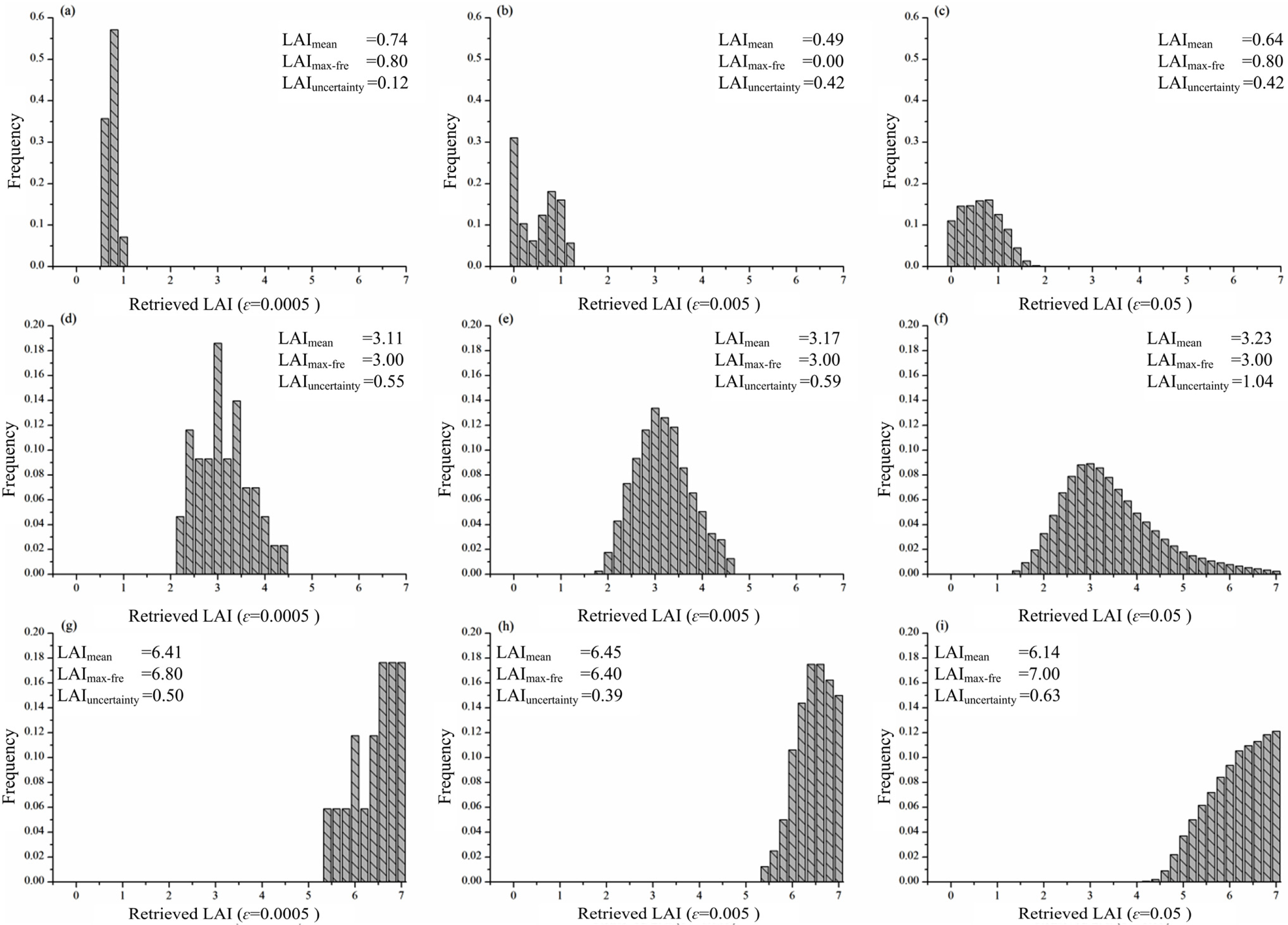
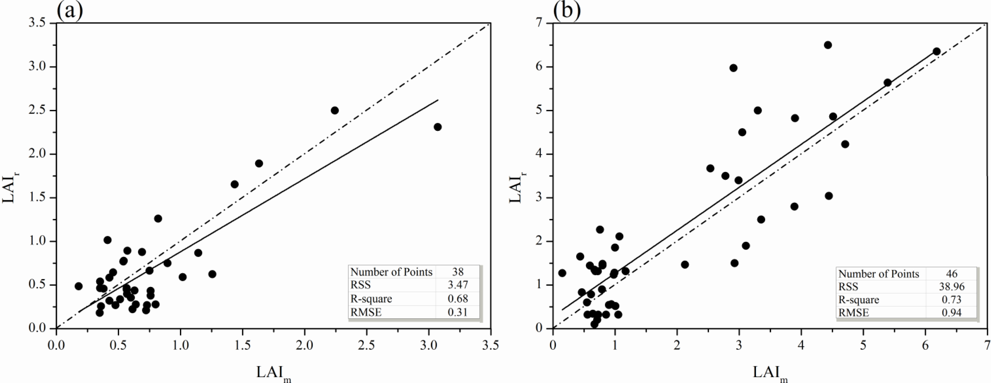
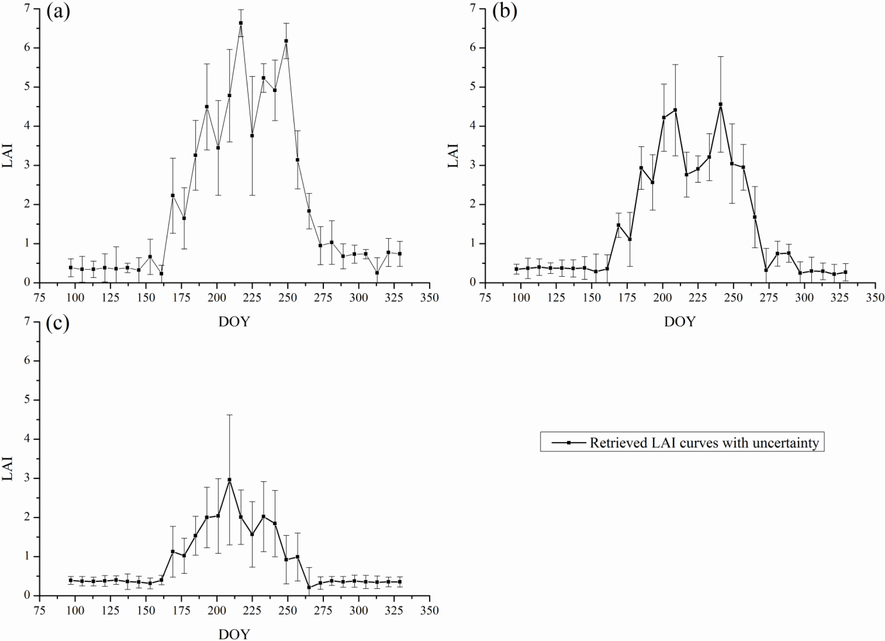
4.2. Retrieved LAI on Each DOY

The NDVI images from DOY 97 to 177 and from DOY 265 to 329 (the arid periods) were used to retrieve relatively lower LAI values, and both the NIR and NDVI images from DOY 185 to 257 were used to retrieve relatively higher LAI values to alleviate the influence of the soil background (Section 2.1.2). As stated in Section 2.1.4, LAI_max-fre was used as the LAI_r, but it may be not reliable at low values of ε. For example, in Figure 4b, LAI_mean was 0.49, whereas LAI_max-fre was 0. This singular case was avoided in Figure 4c, where ε = 0.05. However, if the value of ε was set too high, the retrieval scheme would be meaningless because the uncertainty in the LAI_r values would increase as well (Equation (11)). In Figure 4d–f, as ε increases, the LAI distribution approached a normal distribution. In the case shown in Figure 4f, LAI_mean or LAI_max-fre can be regarded as the LAI_r. However, if the LAI was near the boundaries of the given range, LAI_mean and LAI_max-fre might differ greatly. For example, in Figure 4i, LAI_mean = 6.14, whereas LAI_max-fre = 7.0 because the LAI distribution was no longer normally distributed. In this case, it was more reliable to set LAI_max-fre as the LAI_r, as was assumed in Section 2.1.4. Therefore, in the study, ε = 0.05, and LAI_max-fre was set as the LAI_r.

Figure 5a compares the LAI_r and ground-measured LAI (LAI_m) values from July. The dashed line is the 1:1 line, and the solid line is the least-squares regression line. Of 38 points, the residual sum of squares (RSS), coefficient of determination(R²), and root-mean-square error (RMSE) values were 3.47, 0.68, and 0.31, respectively. Because the points were clustered at low LAI values (≤1.0), the RMSE value of 0.31 could signal a low level of precision of the retrieval. In August (Figure 5b), the LAI_r and LAI_m points at high and low LAI values were less scattered than those in the middle range of LAI values. In other words, the LAI retrieval procedure might be more sensitive at the low and high ends of the LAI values. Of 46 points, the RSS, R², and RMSE values were 38.96, 0.73, and 0.94, respectively. The higher RSS and RMSE values in August compared to those in July could be caused by the increased LAI values as the reeds grew during this part of the year. This interpretation was supported by the high measured LAI values (Figure 5a,b). In summary, the LAI_r values had large uncertainty in the retrieval; this is illustrated in Figure 6, where the peak LAI_r values in the study period and from three pixels (locations) decrease from (a) to (b) to (c). Therefore, the LAI_r values were smoothed to attempt to improve the precision level of LAI_r.

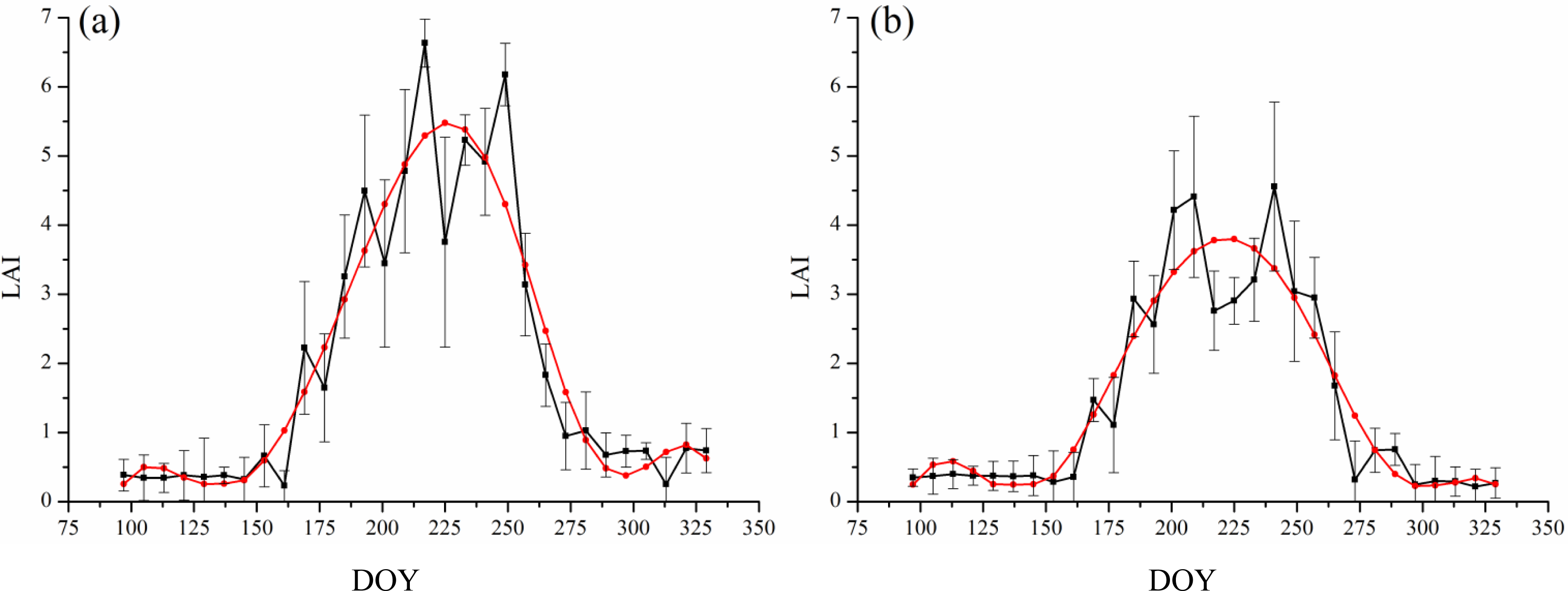
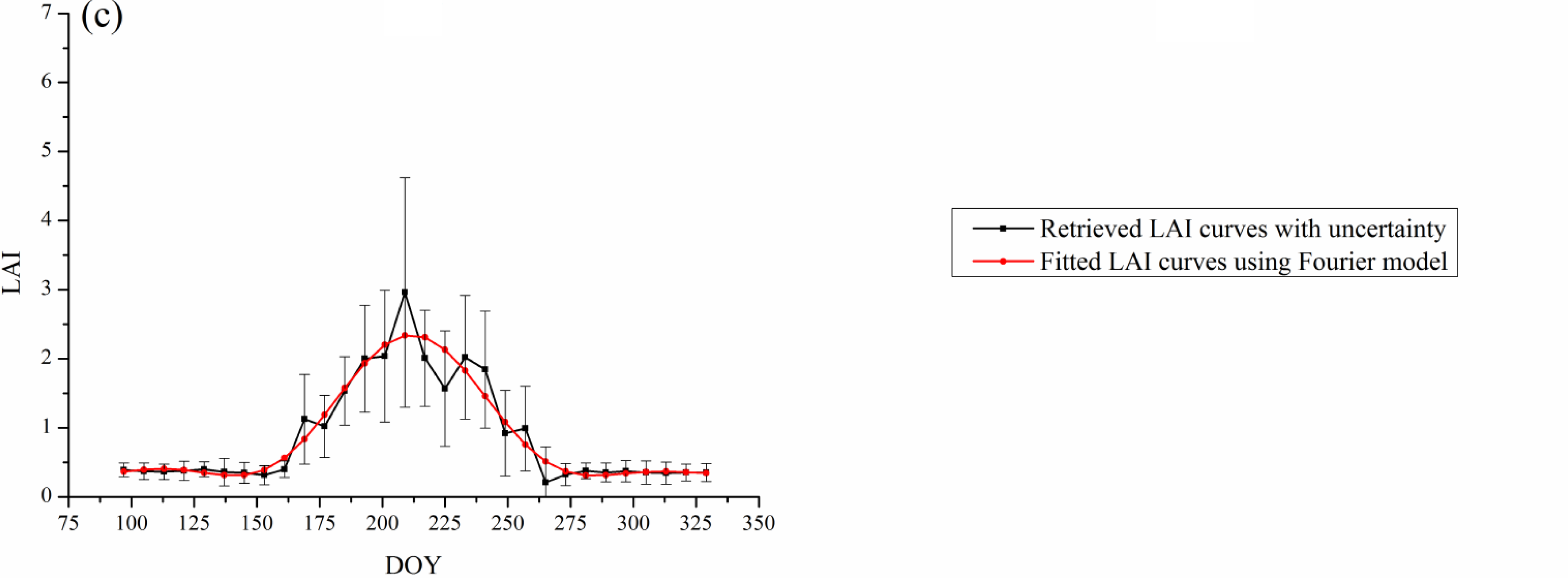
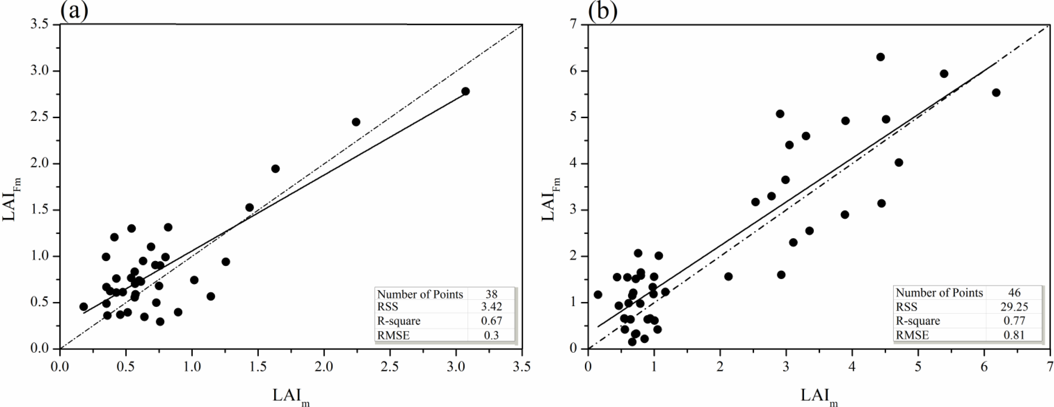
4.3. Smoothing the LAI Curves Using the Fourier Model

As previously discussed, the Fourier model can remove singular points in time series. For example, in Figure 6a,b, the LAI should not decrease from DOY 209 to 241 because the reeds were in the growth stage. In Figure 6c, the decrease in LAI value at DOY 209 could be another singular point. The LAI_r values were then smoothed using the polynomial included in the Fourier model (Equation (14)). Figure 7a–c shows the data from Figure 6a–c after the smoothing that was performed. Clearly, the singular points identified in Figure 6a–c were removed. The LAI fitted by the Fourier model (LAI_F) and LAI_m were then compared again. Of the 38 points from July (Figure 8a), the RSS, R², and RMSE values were 3.42, 0.67, and 0.3, respectively. Of the 46 points from August (Figure 8b), the RSS, R², and RMSE values were 29.25, 0.77, and 0.81, respectively. Compared to the July data, the precision of the LAI_r assessed by the RSS, R², and RMSE values were similar before and after the Fourier model smoothing. No meaningful improvement in the precision was achieved for the LAI_r values. The precision level of the August LAI_r data might have improved after the Fourier smoothing based on the decrease in the RSS and RSME values and the increase in R² value compared with the values before the smoothing, but the improvement was slight. The extended Fourier approach was investigated next to determine whether the approach could increase the precision level in a meaningful way.

4.4. Improving the LAI Curves Using the Extended Fourier Approach

As shown in Figure 9, the LAIr curves were also smoothed using the extended Fourier approach (LAI_eF), but the shapes of the LAI_F and LAI_eF curves were different. The LAI_eF curves were farther away from the LAI_r points with higher uncertainty and were closer to the LAI_r points with lower uncertainty. For example, in Figure 9a, the LAI_r value had a much lower uncertainty on DOY 217 than on DOY 225. The LAI_eF curve was similar to the LAI_r value on DOY 217 but far from that on DOY 225. Figure 9b,c had similar characteristics, but the LAI_F curves did not. The LAI_eF and LAI_m values were then compared again (Figure 10). For the 38 points in July (Figure 10a), the RSS, R², and RMSE values were 3.15, 0.72, and 0.29, respectively. For the 46 points in August (Figure 10b), the RSS, R², and RMSE values were 27.48, 0.79, and 0.78, respectively. The precision level of the LAI_eF values was improved compared with the LAI_r and LAI_F (

Table 3. Levels of precision of LAI_r, LAI_F, and LAI_eF compared to LAI_m on DOY 177 and 233.

		RSS	R-Square	RMSE
DOY 177	LAIr	3.47	0.68	0.31
	LAIF	3.42	0.67	0.30
	LAIeF	3.15	0.72	0.29
DOY 233	LAIr	38.96	0.73	0.94
	LAIF	29.25	0.77	0.81
	LAIeF	27.48	0.79	0.78

). Therefore, the extended Fourier approach not only smoothed the LAI_r curves in the time series but also improved the precision level of the LAI_r values by taking into account the uncertainty in the LAI_r.

5. Discussion

The Fourier model can be used to simulate the variation of LAI values in a time series. The Fourier model includes 11 free variables, which are fitted by the LAI_r at different periods and the least squares method. However, the set of free variables in the Fourier model is much smaller than that in physical dynamic models, such as crop growth models. Physical dynamic models can better simulate the growth of crops because they are structured based on the physical mechanisms of vegetation growth. However, more work needs to be done on the selection of the appropriate model to simulate or approximate the growth of wild plants in alpine wetlands and to determine the large sets of input parameters. Therefore, it is infeasible to use a physical dynamic model to improve LAI estimates.

The Fourier model has been widely used to smooth the curves of parameters that are periodic. However, the model might not improve the precision level of the dataset. In this study, the Fourier model used in the fitting process was extended by taking into account the uncertainty in the LAI_r values. As explained in Section 4.4, the improved fitted curves will be close to the points that have lower uncertainty and avoid points with larger uncertainty. The LAI_r will have the best results and the precision level should be improved. As in the Fourier model, the extended Fourier approach can be used if the dataset is periodic, but the model will improve the precision of the dataset only if the uncertainty in the dataset is expressed correctly.

The LAI_uncertainty imported in Equation (17) is regarded as the uncertainty caused by the ill-posed inversion problem. It can be used as an indicator to represent the uncertainty in the retrieval results as analyzed in Section 2.3. However, it may not describe the absolute uncertainty in the LAI_r values because the uncertainty is affected by many factors, such as cloud cover, the LAI retrieval algorithm, and the ill-posed inversion problem.

6. Concluding Remarks

Characterized by high altitude and cold and dry weather, the alpine wetland is extremely fragile and vulnerable. The vegetation is typically composed of a single type of annual herb. In this study, an extended Fourier approach was presented to improve the LAI_r values in a 2011 time series from an alpine wetland located in western China. The LAI was retrieved on DOYs based on the ACRM, the MYD09Q1 product from DOY 97 to 297, and the LUT algorithm. To alleviate the ill-posed inversion problem, three strategies were implemented. (I) To reduce the influence of the soil background, the NDVI and NIR reflectance of wavebands were used to retrieve the LAI for sparse vegetation and dense vegetation, respectively;(II) A sensitivity analysis of the ACRM in the RED and NIR wavelengths was performed to determine the free parameters using Sobol’s method;(III) The priori information was imported to constrain the range of free parameters in the ACRM. The LAI_r in the time series did not form smooth curves due to the effects of the ill-posed inversion problem. A normalized Fourier model with two additional polynomials was used to smooth the LAI_r curves in the time series because of the periodicity of the vegetation in the study area. The Fourier model is able toimprove the level of precision of the LAI_r if singular points are present, but it may also reduce the level of precision if the datasets that the model is based on contain large uncertainty. An extended Fourier approach was presented by taking into account the uncertainty in the LAI_r in the Fourier model to improve the level of precision of the LAI_r. The LAI_r, LAI_F, and LAI_eF values were validated through a comparison with field measured LAI (LAI_m) values, which resulted in R² values of 0.68, 0.67 and 0.72, RSS values of 3.47, 3.42 and 3.15, and RMSE values of 0.31, 0.30 and 0.29, respectively, on DOY 177 (early July). On DOY 233 (late August), the R² values were 0.73, 0.77 and 0.79, the RSS values were 38.96, 29.25 and 27.48, and the RMSE values were 0.94, 0.81 and 0.78, respectively. The results demonstrated that this approach has the potential to improve the level of precision of periodically varying parameters in a time series.

References

1. Houborg, R.; Soegaard, H.; Boegh, E. Combining vegetation index and model inversion methods for the extraction of key vegetation biophysical parameters using Terra and Aqua MODIS reflectance data. Remote Sens. Environ 2007, 106, 39–58. [Google Scholar]
2. Fensholt, R.; Sandholt, I.; Rasmussen, M.S. Evaluation of MODIS LAI, FAPAR and the relation between FAPAR and NDVI in a semi-arid environment using in situ measurements. Remote Sens. Environ 2004, 91, 490–507. [Google Scholar]
3. Xiao, Z.; Liang, S.; Wang, J.; Jiang, B.; Li, X. Real-time retrieval of leaf area index from MODIS time series data. Remote Sens. Environ 2011, 115, 97–106. [Google Scholar]
4. Darvishzadeh, R.; Skidmore, A.; Schlerf, M.; Atzberger, C. Inversion of a radiative transfer model for estimating vegetation LAI and chlorophyll in a heterogeneous grassland. Remote Sens. Environ 2008, 112, 2592–2604. [Google Scholar]
5. Doraiswamy, P.; Hatfield, J.; Jackson, T.; Akhmedov, B.; Prueger, J.; Stern, A. Crop condition and yield simulations using Landsat and MODIS. Remote Sens. Environ 2004, 92, 548–559. [Google Scholar]
6. Houborg, R.; Anderson, M.; Daughtry, C. Utility of an image-based canopy reflectance modeling tool for remote estimation of LAI and leaf chlorophyll content at the field scale. Remote Sens. Environ 2009, 113, 259–274. [Google Scholar]
7. Meroni, M.; Colombo, R.; Panigada, C. Inversion of a radiative transfer model with hyperspectral observations for LAI mapping in poplar plantations. Remote Sens. Environ 2004, 92, 195–206. [Google Scholar]
8. Colombo, R.; Bellingeri, D.; Fasolini, D.; Marino, C.M. Retrieval of leaf area index in different vegetation types using high resolution satellite data. Remote Sens. Environ 2003, 86, 120–131. [Google Scholar]
9. Combal, B.; Baret, F.; Weiss, M.; Trubuil, A.; Mace, D.; Pragnere, A.; Myneni, R.; Knyazikhin, Y.; Wang, L. Retrieval of canopy biophysical variables from bidirectional reflectance: Using priori information to solve the ill-posed inverse problem. Remote Sens. Environ 2003, 84, 1–15. [Google Scholar]
10. Combal, B.; Baret, F.; Weiss, M. Improving canopy variables estimation from remote sensing data by exploiting ancillary information. Case study on sugar beet canopies. Agronomie 2002, 22, 205–215. [Google Scholar]
11. Hermance, J.F.; Jacob, R.W.; Bradley, B.A.; Mustard, J.F. Extracting phenological signals from multiyear AVHRR NDVI time series: Framework for applying high-order annual splines with roughness damping. IEEE Trans. Geosci. Remote Sens 2007, 45, 3264–3276. [Google Scholar]
12. Moody, A.; Johnson, D.M. Land-surface phenologies from AVHRR using the discrete fourier transform. Remote Sens. Environ. 2001, 75, 305–323. [Google Scholar]
13. Carrão, H.; Gonalves, P.; Caetano, M. A nonlinear harmonic model for fitting satellite image time series: Analysis and prediction of land cover dynamics. IEEE Trans. Geosci. Remote Sens 2010, 48, 1919–1930. [Google Scholar]
14. Roerink, G.; Menenti, M.; Verhoef, W. Reconstructing cloudfree NDVI composites using Fourier analysis of time series. Int. J. Remote Sens. 2000, 21, 1911–1917. [Google Scholar]
15. Geerken, R.; Zaitchik, B.; Evans, J. Classifying rangeland vegetation type and coverage from NDVI time series using Fourier filtered cycle similarity. Int. J. Remote Sens. 2005, 26, 5535–5554. [Google Scholar]
16. Brooks, E.B.; Thomas, V.A.; Wynne, R.H.; Coulston, J.W. Fitting the multitemporal curve: A fourier series approach to the missing data problem in remote sensing analysis. IEEE Trans. Geosci. Remote Sens. 2012, 50, 3340–3353. [Google Scholar]
17. Bach, H.; Mauser, W. Methods and examples for remote sensing data assimilation in land surface process modeling. IEEE Trans. Geosci. Remote Sens. 2003, 41, 1629–1637. [Google Scholar]
18. Seo, D.-J.; Cajina, L.; Corby, R.; Howieson, T. Automatic state updating for operational streamflow forecasting via variational data assimilation. J. Hydrol. 2009, 367, 255–275. [Google Scholar]
19. Naud, C.; Makowski, D.; Jeuffroy, M.-H. Application of an interacting particle filter to improve nitrogen nutrition index predictions for winter wheat. Ecol. Model. 2007, 207, 251–263. [Google Scholar]
20. Van Leeuwen, P.J. A variance-minimizing filter for large-scale applications. Mon. Wea. Rev. 2003, 131, 2071–2084. [Google Scholar]
21. Smith, P.J.; Dance, S.L.; Nichols, N.K. A hybrid data assimilation scheme for model parameter estimation: Application to morphodynamic modelling. Comput. Fluids 2011, 46, 436–441. [Google Scholar]
22. Van Velzen, N.; Segers, A. A problem-solving environment for data assimilation in air quality modelling. Environ. Model. Softw. 2010, 25, 277–288. [Google Scholar]
23. Rudd, A.; Roulstone, I.; Eyre, J. A simple column model to explore anticipated problems in variational assimilation of satellite observations. Environ. Model. Softw. 2012, 27, 23–39. [Google Scholar] [Green Version]
24. Tripathy, R.; Chaudhari, K.N.; Mukherjee, J.; Ray, S.S.; Patel, N.; Panigrahy, S.; Parihar, J.S. Forecasting wheat yield in Punjab state of India by combining crop simulation model WOFOST and remotely sensed inputs. Remote Sens. Lett. 2012, 4, 19–28. [Google Scholar]
25. Confalonieri, R.; Acutis, M.; Bellocchi, G.; Donatelli, M. Multi-metric evaluation of the models WARM, CropSyst, and WOFOST for rice. Ecol. Model. 2009, 220, 1395–1410. [Google Scholar]
26. Marin, F.R.; Jones, J.W.; Royce, F.; Suguitani, C.; Donzeli, J.L.; Wander Filho, J.P.; Nassif, D.S.P. Parameterization and evaluation of predictions of DSSAT/CANEGRO for brazilian sugarcane. Agron. J. 2011, 103, 304–315. [Google Scholar]
27. Van Dam, J.C.; Groenendijk, P.; Hendriks, R.F.A.; Kroes, J.G. Advances of modeling water flow in variably saturated soils with swap. Vadose Zone J. 2008, 7, 640–653. [Google Scholar]
28. Kalnay, E.; Li, H.; Miyoshi, T.; Yang, S.C.; Ballabrera-poy, J. 4-D-Var or ensemble kalman filter? Tellus A 2007, 59, 758–773. [Google Scholar]
29. Jakubauskas, M.E.; Legates, D.R.; Kastens, J.H. Harmonic analysis of time-series AVHRR NDVI data. Photogramm. Eng. Remote Sens. 2001, 67, 461–470. [Google Scholar]
30. Hermance, J.F. Stabilizing high-order, non-classical harmonic analysis of NDVI data for average annual models by damping model roughness. Int. J. Remote Sens. 2007, 28, 2801–2819. [Google Scholar]
31. Tucker, C.J. Red and photographic infrared linear combinations for monitoring vegetation. Remote Sens. Environ. 1979, 8, 127–150. [Google Scholar]
32. Sobol, I.M. Sensitivity estimates for nonlinear mathematical models. Math. Model. Comput. Exp. 1993, 1, 407–414. [Google Scholar]
33. Kuusk, A. A two-layer canopy reflectance model. J. Quant. Spectrosc. Radiat. Transf. 2001, 71, 1–9. [Google Scholar]
34. Iqbal, M. An Introduction to Solar Radiation; Academic Press: Toronto, ON, Canada, 1983. [Google Scholar]
35. Price, J.C. On the information content of soil reflectance spectra. Remote Sens. Environ. 1990, 33, 113–121. [Google Scholar]
36. Kuusk, A. A multispectral canopy reflectance model. Remote Sens. Environ. 1994, 50, 75–82. [Google Scholar]
37. Campbell, G. Derivation of an angle density function for canopies with ellipsoidal leaf angle distributions. Agric. For. Meteorol. 1990, 49, 173–176. [Google Scholar]
38. Liang, S. Quantitative Remote Sensing of Land Surfaces; John Wiley and Sons, Inc: New York, NY, USA, 2004. [Google Scholar]
39. Kuusk, A. A Markov chain model of canopy reflectance. Agric. For. Meteorol. 1995, 76, 221–236. [Google Scholar]
40. Jacquemoud, S.; Baret, F. Prospect: A model of leaf optical properties spectra. Remote Sens. Environ 1990, 34, 75–91. [Google Scholar]
41. Nossent, J.; Elsen, P.; Bauwens, W. Sobol’sensitivity analysis of a complex environmental model. Environ. Model. Softw 2011, 26, 1515–1525. [Google Scholar]
42. Glen, G.; Isaacs, K. Estimating sobol sensitivity indices using correlations. Environ. Model. Softw 2012, 37, 157–166. [Google Scholar]
43. Homma, T.; Saltelli, A. Importance measures in global sensitivity analysis of nonlinear models. Reliab. Eng. Syst. Saf 1996, 52, 1–17. [Google Scholar]
44. He, B.; Quan, X.; Xing, M. Retrieval of leaf area index in alpine wetlands using a two-layer canopy reflectance model. Int. J. Appl. Earth Obs. Geoinf 2013, 21, 78–91. [Google Scholar]
45. Verhoef, W.; Bach, H. Simulation of hyperspectral and directional radiance images using coupled biophysical and atmospheric radiative transfer models. Remote Sens. Environ 2003, 87, 23–41. [Google Scholar]
Figure 1. Sensitivity of normalized difference vegetation index (NDVI) to leaf area index (LAI) (a) and of NIR reflectance to LAI (b) by running two-layer canopy reflectance model (ACRM) forward at different values of s1.
Remotesensing 06 01171f1
Figure 2. The study area (Wutumeiren prairie). The color composite Landsat5 image is TM4 (red), TM3 (green), and TM2 (blue). Green points represent the sampling plots from 6 to 9 July 2011, and the yellow points represent sampling plots between 26 and 29 August 2011.
Remotesensing 06 01171f2
Figure 3. Sensitivity analysis of key input parameters of ACRM at near-infrared (NIR) and RED wavebands using Sobol’s method. TSI stands for total sensitivity index.
Remotesensing 06 01171f3
Figure 4. Distribution of LAIr. Because of the ill-posed inversion problem, LAIr is not a single value but a wide range of different frequencies.
Remotesensing 06 01171f4
Figure 5. LAIr compared to the field-measured LAI on DOY 177 (July) (a) and DOY 233 (August) (b) in 2011.
Remotesensing 06 01171f5
Figure 6. LAIr versus day of year (DOY) for three pixels. The solid line is the LAIr, and the error bars on each DOY represent LAIuncertainty. (a) and (b) are the LAIr of vegetation near Wutumeiren river; (c) is the LAIr of vegetation in drought area. The peak LAIr values in the study period decrease from (a) to (b) to (c).
Remotesensing 06 01171f6
Figure 7. Comparison of the LAIr and LAIF for three pixels from dense vegetation to sparse vegetation in the time series. (a) and (b) are the LAIr of vegetation near Wutumeiren river; (c) is the LAIr of vegetation in drought area.
Remotesensing 06 01171f7aRemotesensing 06 01171f7b
Figure 8. Results of LAIF compared to LAIr in early July (a) and late August (b) 2011.
Remotesensing 06 01171f8
Figure 9. Comparison between the LAIr, LAIF, and LAIeF values of three pixels from dense vegetation to sparse vegetation in the time series. (a) and (b) are the LAIr of vegetation near Wutumeiren river; (c) is the LAIr of vegetation in drought area.
Remotesensing 06 01171f9
Figure 10. Results of the LAIeF values compared to the LAIm values in early July (a) and late August (b) 2011.
Remotesensing 06 01171f10