Multi-Polarization ASAR Backscattering from Herbaceous Wetlands in Poyang Lake Region, China


Abstract
: Wetlands are one of the most important ecosystems on Earth. There is an urgent need to quantify the biophysical parameters (e.g., plant height, aboveground biomass) and map total remaining areas of wetlands in order to evaluate the ecological status of wetlands. In this study, Environmental Satellite/Advanced Synthetic Aperture Radar (ENVISAT/ASAR) dual-polarization C-band data acquired in 2005 is tested to investigate radar backscattering mechanisms with the variation of hydrological conditions during the growing cycle of two types of herbaceous wetland species, which colonize lake borders with different elevation in Poyang Lake region, China. Phragmites communis (L.) Trin. is semi-aquatic emergent vegetation with vertical stem and blade-like leaves, and the emergent Carex spp. has rhizome and long leaves. In this study, the potential of ASAR data in HH-, HV-, and VV-polarization in mapping different wetland types is examined, by observing their dynamic variations throughout the whole flooding cycle. The sensitivity of ASAR backscattering coefficients to vegetation parameters of plant height, fresh and dry biomass, and vegetation water content is also analyzed for Phragmites communis (L.) Trin. and Carex spp. The research for Phragmites communis (L.) Trin. shows that HH polarization is more sensitive to plant height and dry biomass than HV polarization. ASAR backscattering coefficients are relatively less sensitive to fresh biomass, especially in HV polarization. However, both are highly dependent on canopy water content. In contrast, the dependence of HH- and HV- backscattering from Carex community on vegetation parameters is poor, and the radar backscattering mechanism is controlled by ground water level.1. Introduction
Wetlands are among Earth’s most productive systems. These ecosystems fix and store organic matter, and release dissolved and particulate organic carbon to adjacent aquatic environments or down streams [1]. Their contribution to carbon sequestration is highlighted by the fact that wetlands occupy 4%–5% of the land area of the globe, yet hold approximately 20% of the carbon in the terrestrial biosphere [2]. The productivity of many wetland plants is as great as they are the most hearty agricultural crops [3]. This type of ecosystem is currently a small, persistent sink for carbon dioxide (CO2) and a large source of methane (CH4) [4]. Natural and agricultural wetlands together contribute over 40% of the annual atmospheric emissions of CH4 and are therefore considered to be the largest single contributor of this gas to the troposphere [5]. The extent of wetlands is uncertain due to the difficulty of identifying and classifying wetlands on a global scale, the estimates of global wetlands vary from 5.3 × 10¹² m2 [6] to 8.6 × 10¹² m2 [3]. Therefore, it is urgent to quantify the biophysical parameters (e.g., plant height, aboveground biomass, leaf area index) and total remaining areas of wetlands in order to evaluate the ecological status of wetlands. In addition to in situ measurements and monitoring activities over the wetlands, satellite remote sensing may provide a time-saving alternative for continuously monitoring and evaluating biophysical parameters of wetlands.
Active microwave radar is one of the most important remote sensing tools for mapping wetlands. The launch of the SeaSAT Synthetic Aperture Radar (SAR) in 1978 initiated the technology of active microwave radar for wetland studies [7]. Multi-band and full polarimetric Shuttle Imaging Radar-C (SIR-C) proved to be useful in detecting seasonal inundation extents, flooding cycles, and the changes in water level, as well as mapping different wetland species [8–14]. SAR data from single frequency radar (JERS-1 and RADARSAT) were successfully used for monitoring and mapping wetlands in the Amazon floodplain and in Florida, USA [15–19]. Other researchers used ERS-1, ERS-2 and RADARSAT data for mapping paddy rice crops and wetlands, as well as estimating soil moisture and seasonal hydrologic and biophysical properties [20–23]. With the launch of ENVISAT-ASAR in 2002, satellite-borne SAR sensor with multiple or full polarizations became available, which have more potential for wetlands research, including flooding extent description, wetland species monitoring and mapping, and the retrieval of wetland vegetation biophysical parameters [24–36].
Understanding the capabilities of imaging radar to monitor and map wetland ecosystems requires knowledge of microwave scattering from vegetated surfaces. The fundamental characteristic recorded on a radar image is the spatial variation in the radar backscattering coefficient. To understand radar scattering from complex vegetation covers, it is necessary to think in terms of the different canopy layers affecting the radar signature [37]. Generally, two sets of factors exert primary control over radar backscattering: (1) geometrical factors relating to structural attributes of the surface and any overlying vegetation-cover relative to sensor parameters of wavelength and viewing geometry; and (2) electrical factors determined by the relative dielectric constants of soil and vegetation at a given wavelength [38]. Radar backscattering mechanism in wetlands includes vegetation canopy volume scattering, ground/water surface scattering, and the multiple interactions between canopy and ground/water surface. The dynamic change of hydrology conditions makes radar backscattering mechanism more complicated in wetland ecosystems. The dominant scattering mechanism may change from canopy volume scattering to double bounce, or even to specular reflection with the variation of ground water depth. SAR images are also used to characterize ecosystem structure, including biophysical parameters such as plant height, volume density, and vegetation biomass [33,35,39–44]. The sensitivity of incident microwave depends on vegetation structure or vegetation species. C-band VV-polarized ERS SAR data were successfully used to invert dry biomass of Andean herbaceous wetland vegetation. The accuracy for spatial estimation of biomass was within the range of 1 kg/m2 to 2 kg/m2 of dry biomass, meeting the requirement of rangeland management purposes [39]. ERS SAR backscattering coefficients are significantly correlated with plant height (R2 = 0.93) and fresh biomass of paddy rice (R2 = 0.96) [22]. Compared with predictions from the MIMICS theoretical model, no apparent relationship is observed between aboveground biomass in south Florida wetlands and ERS-SAR backscattering coefficients due to the short vegetation and small size of marl prairie [21]. C-band RADARSAT data is also proven to be highly sensitive to plant structural parameters [45]. Compared with C-band SAR data, L-band SAR signal has more potential in flooding monitoring in forested wetlands, and can improve saturated point of vegetation biomass [8,11,31,46,47]. Longer wavelength of L-band radar signals could penetrate forest canopy to detect surface ground soil or water, while X- and C-band backscattering signals mainly come from canopy branches and leaves. The latter two bands are more appropriate in studying herbaceous wetlands vegetation [29,48]. L-band JERS-1 has higher saturation point of biomass than C-band RADARSAT for estimating above-water biomass of aquatic vegetation in the Amazon floodplain, and the integration of the L-band and C-band provided the best correlation and an intermediate saturation point [15].
In this study, C-band ENVISAT/ASAR fine resolution images with multiple polarizations are used along with field measurements to monitor two wetlands communities with different structure. The objective of this study is twofold: (1) investigate the temporal variability of ASAR backscattering coefficients and radar backscattering mechanisms from two wetland communities; and (2) understand the relationships between radar backscattering coefficients in HH and HV polarization and the biophysical characteristics (plant height and aboveground biomass) of wetland species.
2. Brief Description of the Study Area
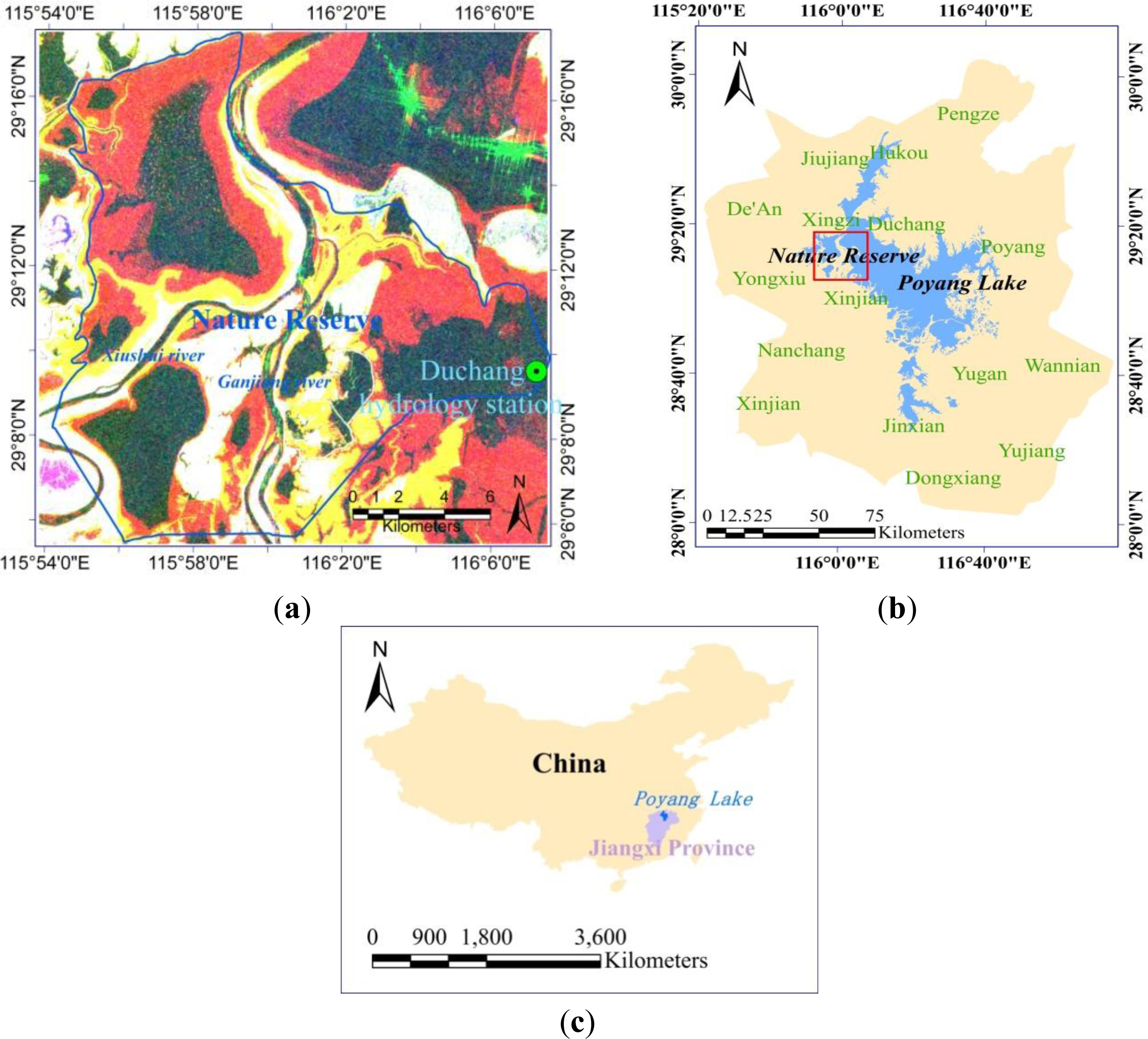
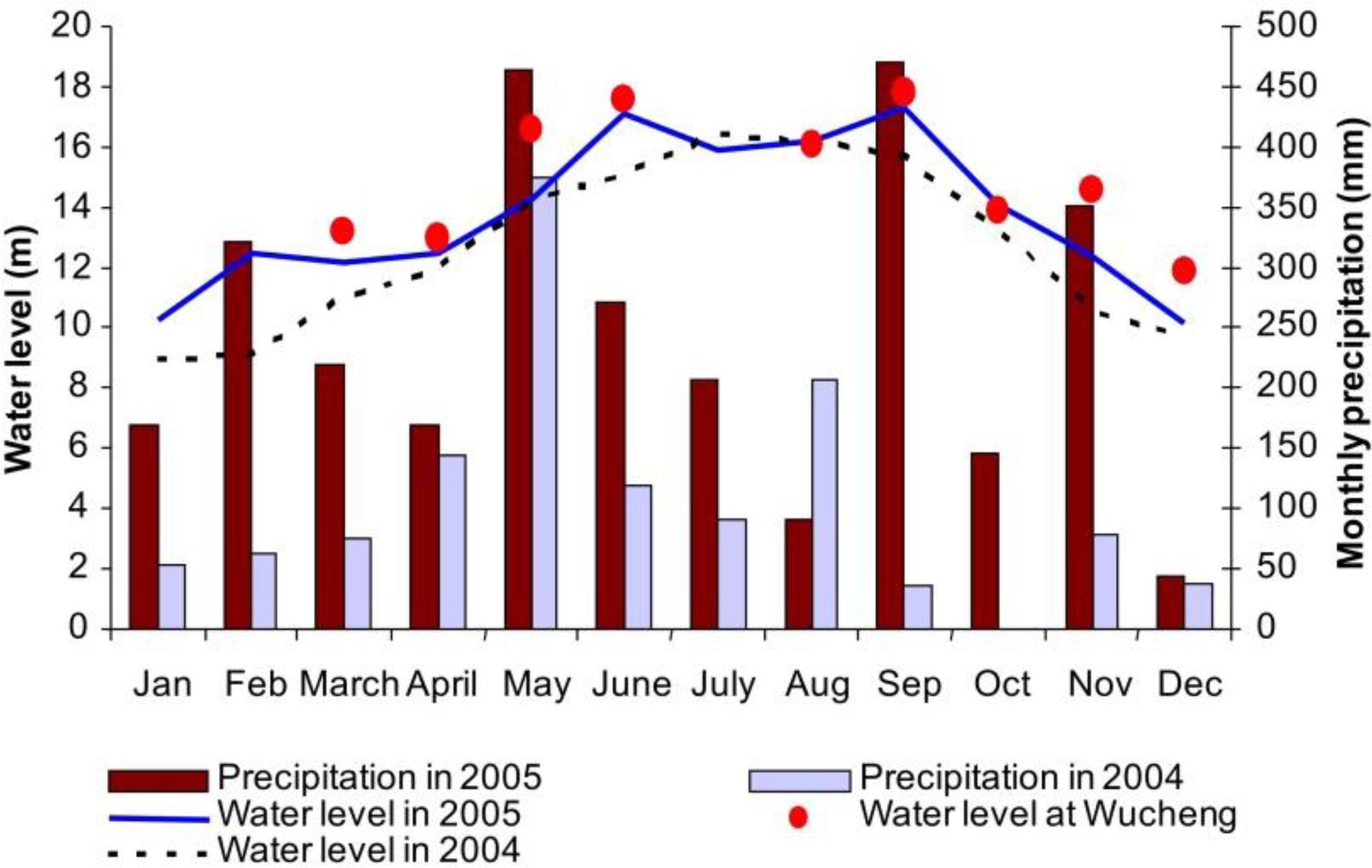
The study area is located at the Poyang Lake National Nature Reserve, situated northwest of Poyang Lake in Jiangxi Province (29°05′∼29°17′N and 115°54′∼116°08′E), China (Figure 1). The subtropical monsoon climate is characterized by distinct dry and rainy seasons in the Poyang Lake region. The rainy season begins in early April, when the southeast monsoon starts to influence this region. Annual precipitation is about 1482 mm, but precipitation varies significantly between months and years. Maximum precipitation occurs in June, accounting for over 17% of annual precipitation, whereas minimum precipitation in December is only 42 mm (Figure 2). Influenced by both summer monsoon and winter monsoon, four distinct seasons exist in this region. Generally, the annual mean temperature is about 25 °C, with highest monthly mean temperature occurring in July (29.4 °C) and the lowest in January (4.8 °C) [49].
Poyang Lake plays an important role in regional flooding control and water resource management. Five rivers (Gangjiang, Xiushui, Raohe, Xinjiang and Fuhe) flow into different parts of Poyang Lake. As it is connected to downstream Yangtze River, the flooding pattern of Poyang Lake is influenced not only by local precipitation and water source from the five rivers, but also by the backflows from Yangtze River. Thus, the flooding pattern in the lake varies from area to area and from year to year. The rivers of Gangjiang and Xiushui join at the town of Wucheng, and both are responsible for the varying water levels in the study area. Water-level and precipitation data in 2004 and 2005 were collected at the Duchang hydrology station (Figure 2). The year 2005 was a rainy year with annual precipitation of 2916 mm, approximately 130% higher than annual precipitation in 2004. A unimodal cycle of water level fluctuation was observed in 2004, and the highest and lowest water levels occurred in July and January, respectively. By comparison, two flooding peaks occurred in June and September 2005, due to incoming water from the five rivers and reverse water flow from the lower Yangtze River. The available nearest water level data was collected at the Wucheng hydrology station on the dates when ASAR data were acquired, which provided more accurate information of water level (red dots in Figure 2). Two flooding peaks also occurred, which dominated the growing status of wetland vegetation in the study area.
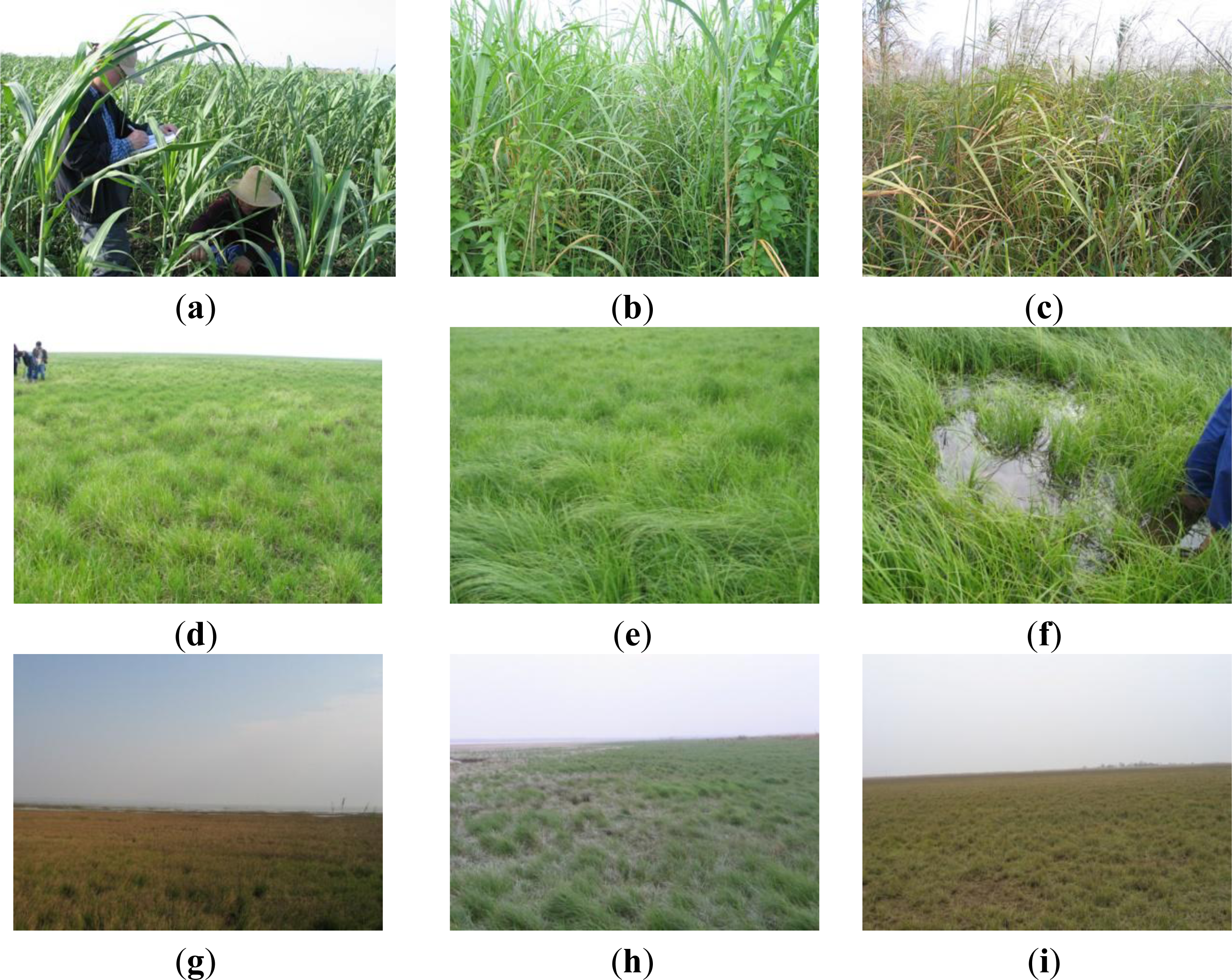
Wetland vegetation in Poyang Lake includes herbaceous vegetation that has adapted to local water conditions. From the lake center to the shorelines, wetland vegetation is zonally distributed, depending on water levels and environmental conditions. This includes floating vegetation, submerged vegetation (e.g., Potamogeton malainus and Vallisneria spiralis), emergent aquatic vegetation (e.g., Carex spp.), and semi-aquatic emergent tall vegetation, (e.g., Phragmites communis, Miscanthus sacchariflorus, and Zizania caduciflora).
Main Carex spp. growing in the Poyang Lake Nature Reserve includes Carex cinerascens, Carex argyi, and Carex unisexualis, others such as Carex laticeps and Carex doniana are also observed in this study area (Figure 3d–i). Carex plants dominate Poyang Lake wetlands, and colonize those areas with the elevation between 14.2 m and 16 m. This community can grow both in shallow water and wet soil, and annual inundation period ranges between 160 and 200 days. The meadow bog soil under this community containing about 30% clay can keep water and provide good growth conditions. New shoots sprout from underground creeping stems in late February or early March, and grow rapidly in April and May. This species starts to be inundated under water from May during the peak flooding period. Another growing cycle begins after water level recedes in autumn, but its growth slows down and eventually stops in winter due to cold temperature. Carex spp. communities provide ideal habitats and food for migratory birds. Furthermore, as one of the most important grazing resources in the Poyang Lake region for livestock (e.g., cattle), the plant growing condition and productivity of Carex species affect the development of livestock husbandry. Therefore, mapping the dynamic distribution of Carex species is important for both ecological protection and local economic development.
The areas colonized by Phragmites communis have been reduced significantly in recent years due to anthropogenic influences [50,51]. Only a narrow Phragmites communis zone exists along the shoreline of Xiushui River at Dahuchi Lake; usually mixes of M. sacchariflorus, Polygonum spp., and Artenlisia Julagaris. Since Phragmites spp. colonizes the higher wetlands areas, the flooding duration lasts at most two or three months. The ground meadow soil contains an abundance of fine silt and sand with high perviousness and provides good growth conditions for Phragmites communis. Generally, the life cycle of Phragmites communis plants is divided into four periods: the regrowth period (March to May), the maturity period (June to September), the flowering period, and the senescent period. Burning of dead Phragmites communis often occurs in winter or early spring, and burn scars were observed in March 2005 during field surveys. Plant height increases 3 cm to 6 cm every day in April and May and reaches up to 3 m in summer. Feathery and plume-like flowers appear in October. The growth cycle ends in December due to cold weather and lack of water (Figure 3a–c). As one of the most important wetland communities in the Poyang Lake, Phragmites communis wetlands not only provide food and habitat for wintering migratory birds, their tall height and colonization along the shoreline also protect the wintering birds from human interferences [50,51]. However, the quality and quantity of this wetland community has decreased significantly over the past half century due to overgrazing/over-harvesting and plowing to exterminate schistosome. In recent years, young poplar plants were introduced and have been invading on Phragmites communis community.
3. Field Data
Field surveys and samplings were conducted in spring and autumn 2005 following the acquisition of ENVISAT/ASAR data (Table 1). The field work focused on the emergent aquatic and semi-aquatic vegetation including Carex spp. and Phragmites communis in the Poyang Lake Nature Reserve. For sampling design, the zonal distribution of wetland vegetation along the profile of lakes corresponding to the variation of elevation was considered, and thus field sampling was conducted perpendicular to vegetation zones to collect different vegetation species with different growing status, and parallel to lake shore to collect more samples from the same community. Considering the vegetation zones are narrow as a result of high dynamics of hydrological conditions along the profile, the perpendicular distance of each sample was over 120 m in average and the parallel distance was over 200 m. The samples were collected from those homogeneous areas, but encompassed various growing stages due to natural vegetation succession and anthropogenic interference. Sample plots were located at different vegetation zones, separated around over hundreds of meters from each other.
At each sampling plot, both soil and vegetation samples were collected. Field measurements include soil wet weight, vegetation species, vegetation fresh weight, vegetation height and percent cover, in addition to photos and GPS-based geographic coordinates. Plants were clipped at their base, weighed for a fresh weight measurement. Soil and vegetation samples were dried in the oven under 85 °C to get constant dry weight. The plot size of vegetation sampling was 0.5 × 0.5 m2 for dense vegetation with greater than 85% cover or 1 × 1 m2 for sparse vegetation. Above ground or above water average plant height was measured in situ, and other parameters were calculated in laboratory. Over sixty samples from Carex community were collected from March to December in 2005, covering two growing cycles in different flooding extent. The zone colonized by Phragmites communis was very narrow (less than 200 m width), which increases the difficulties of sampling. Three sub-sampling plots of the size 0.5 m × 0.5 m and/or 1 m × 1 m were randomly distributed across the main sampling site of 150 m × 150 m. These sub-sampling plots were used to calculate averaged biomass and other vegetation parameters for that site. The vegetation parameters of the sub-samples were used to calculate mean value of the main site for establishing the relationships between biophysical parameters and radar backscattering coefficients in the study area. In this study, Vegetation Gravimetric Moisture Content (Mg) [21] is used to calculate vegetation water content:
4. ENVISAT/ASAR Data Acquisition and Processing
4.1. ENVISAT/ASAR Data and Image Preprocessing
ENVISAT/ASAR, operating at C-band with a frequency of 5.33 GHz, is an advanced version of the SAR system beyond the ERS-1 and ERS-2 sensors. There are 7 swaths (IS1∼IS7) which can be selected at different incident angles ranging from 15° to 45° for fine resolution imagery (12.5 m pixel size). In this study, 10 ASAR scenes in Alternating Polarization Precision (APP) mode (HH/HV or HH/VV) or Image (IM) mode (HH) from swath IS4 to IS7 were acquired (Table 2) between March and November 2005. These SAR images cover the plant growing cycle and one hydrological cycle in Poyang Lake.
Ortho-rectification, speckle filtering and radiometric calibration of the images are pre-requisite steps for deriving backscattering coefficients. Ortho-rectification is conducted using the Ortho-Engine module developed in PCI Geomatics (version 9.0). The Doppler Orbitography and Radio-positioning Integrated by Satellite (DORIS) microwave tracking system carried on ENVISAT provides accurate orbital information about the satellite, which is included in data header file. The PCI Ortho-Engine module utilizes this information together with digital elevation data (DEM) data to develop an ortho-rectification algorithm, and RMS position error is limited to less than 1 pixel [52]. In this study, the DEM data is digitized from a 1:50,000 terrain map of the Poyang Lake region and re-sampled to 12.5 m resolution (the pixel size of ASAR images) in Universal Transverse Mercator (UTM) World Geographical System (WGS) 84 projection of zone 50. In addition, Gamma-MAP filtering is applied to reduce speckles within a 5-by-5 pixel window [53].
4.2. Derivation of Backscattering Coefficients
ASAR level 1b precision image products are provided with radar backscattering recorded as amplitude values, and need to be calibrated to backscattering coefficients for multi-temporal SAR image analysis [54]:
For the distributed target (for instance, vegetation), the backscattering coefficients from an Area of Interest (AOI) should be further averaged, in order to reduce radiometric resolution error due to speckles [54]:
5. Results and Discussion
5.1. Temporal Dynamics of Phragmites Communis
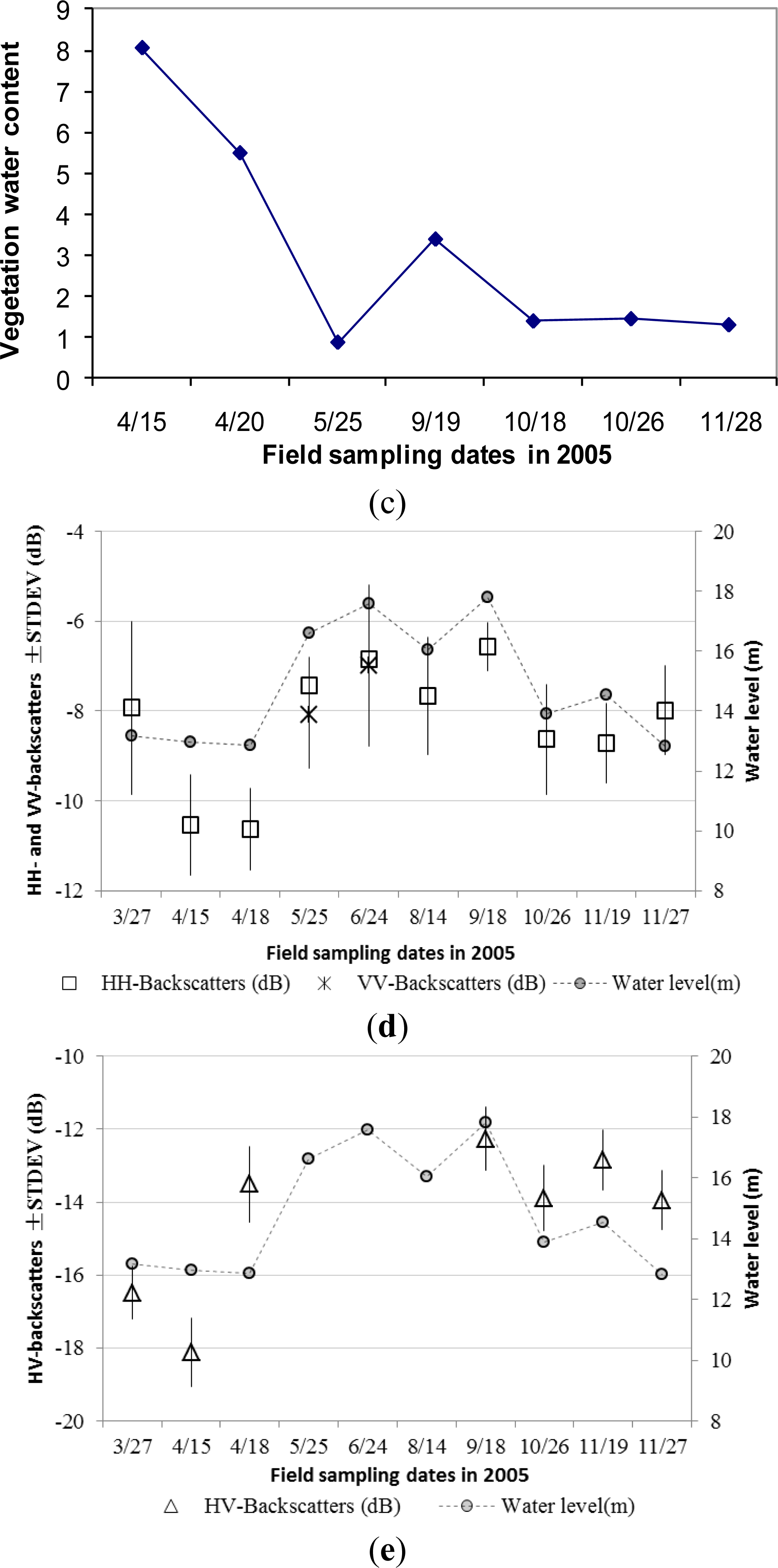
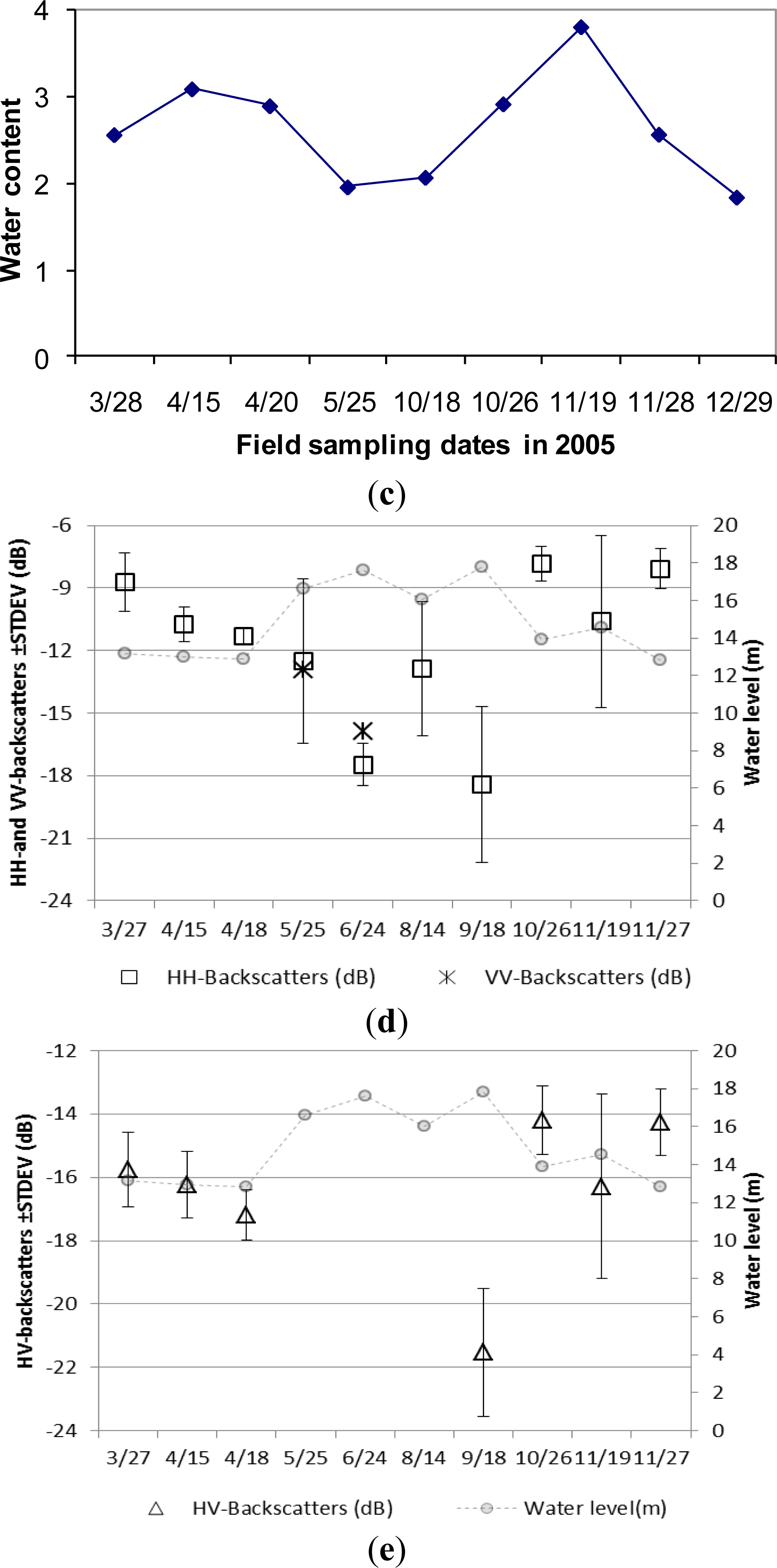
The vegetation initiation (sprouting) of the Phragmites communis starts in late March or early April. Although fresh biomass reached over 1000 g/m2 and plants height reached over 100 cm on 15 April (Figure 4), canopy coverage was about 10% (Table 1). It grew rapidly during early growing stage in rainy season, and the plant height reached over 150 cm within 40 days from middle April to late May (Figures 3 and 4). Ground surface mechanism governs radar backscattering at early growing period, and canopy volume scattering makes a slight contribution to HH-backscattering. HH-backscattering coefficient observed on 27 March was higher over 2 dB than on 15 April, due to wetter soil affected by precipitation on that date (Table 2, Figure 4d). However, HH-polarized ASAR backscattering had no clear change from 15 to 18 in April, though plant height and biomass increased noticeably. This further indicates that variation of radar backscattering coefficients is mainly controlled by soil moisture during this period. The low rainfall on 18 April did not change soil moisture much, and thus had no effect on observed HH-backscattering. In contrast, HV polarization was more sensitive to plant structure and biomass. HV-backscattering coefficient increased almost 5 dB in three days from 15 to 18 in April (Table 2, Figure 4e). The dominant scattering mechanism in HV polarization changed from surface ground scattering to vegetation canopy volume scattering in April, and the multiple interactions between vegetation canopy and ground surface should not be ignored in this stage.
The peak height over 2.5 m was observed on date of 25 May 2005 during its late vegetative re-growth period. The plant height was gradually reduced to less than 2 m from the maturity period to the senescence period because plant stems started to bend in this stage. Seasonal dynamics of fresh biomass and dry biomass were similar to plants height (Figure 4b). The observed maximums of fresh and dry biomass also occurred in late May of 5200 g/m2 and 2770 g/m2 respectively. With the increase of plant height and biomass, HH-backscattering coefficients increased by 3 dB from middle April to late May, and the radar backscattering mechanism at C-band was likely to be dominated by canopy volume scattering (Figure 4d). Considering the fast increase in plant height, biomass and canopy coverage, ground surface scattering in HH-, HV-, and VV-polarization contributed little from late April to May, although ground soil was saturated or even partly flooded.
The observed water level on 24 June was close to that on 18 September, the ground surface of Phragmites communis may also be flooded. The multiple interactions between canopy layer and ground water surface increased and played a significant role in radar backscattering mechanism in HH- and VV-polarization from late May to June. During the maturity period from June to September, the canopy was fully developed, and fresh biomass and canopy water content started to drop. Considering the deep penetration ability of HH polarized radar signals, the rise of HH-backscattering on 24 June and 18 September were attributed to the partly flooded ground surface with shallow water depth (less than 5 cm) or wet soil during the high water level stage, which enhanced the multiple interactions of microwaves between the canopy and ground surface. Volume scattering is still the most dominant mechanism, but the multiple interactions between canopy and ground surface cannot be ignored. The higher value of the C-band HH-backscattering coefficients on these two dates (about −7 dB) suggests a double bounce mechanism, when above water canopy drop significantly (Figure 4d). It was assumed that double bounce in VV polarization also occurred by observing its higher standard deviation on 25 June. The high value of HV-backscattering coefficient shows that the multiple interactions between canopy and water surface contributed significantly to radar backscattering mechanism on 18 September. However, HV polarization is not available from May to August, and the controlling scattering mechanism is uncertain.
The leaves and stems of Phragmites communis started to wither with an approaching winter, and, as a result, the fresh biomass and dry biomass reduced to less than 2260 g/m2 and 1380 g/m2, respectively. The observed reduction of plant biomass was also partly ascribed to the destruction from water buffalos grazing on lower-layer and young grasses. Vegetation water content continuously reduced from 88% in the early growing period to 35% in the senescence period (Figure 4c). Although the plant flower head appeared after October, its effect on ASAR backscattering coefficients was not distinctive, and the ASAR backscattering coefficients continued to decline as a result of the reduction in plant biomass and height. With a reduction of canopy coverage during the senescence period, the attenuation of vegetation canopy further decreased, thus direct surface scattering made a larger contribution to the radar backscattering mechanisms.
5.2. Temporal Dynamics of Carex spp
The growing status of Carex spp. is mainly controlled by ground water and weather (temperature) conditions. The soil moisture content data in this community is listed in Table 1. Soil moisture of Carex spp. varies from standing water to almost saturation (with volumetric moisture content of over 0.65) with the increase of elevation. Above ground/water height, fresh and dry biomass, and vegetation water content through the whole year are presented in Figure 5. The field surveying work covers two growing cycles of Carex spp. in spring (from March to May) and autumn (from October to December) respectively. The growing status of Carex spp. in spring is much better than that in autumn, because of good water and temperature condition. Large growing rates occurred in April and November, but the increase of ground water level caused the reduction of above water biomass after middle April.
ASAR backscattering mechanism from Carex spp. is more complex than from Phragmites communis Trin., because this community is distributed over an elevation gradient of 14 to 16 m. Plant height, biomass, soil moisture condition and ground water depth when flooded vary noticeably even on the same date. Canopy layer volume scattering, ground surface scattering and the multiple interactions between them should be quantitatively analyzed according to the variation of vegetation growing stage. Generally, surface scattering controls ASAR backscattering mechanism in HH and HV polarization from Carex community during its early growing stage in March. Canopy volume scattering replaces the role of ground surface, and the multiple interactions between canopy and ground also increases, with the raise of plant height and biomass. However, the increase of canopy coverage and density attenuates the penetration depth of C-band signals, and reduces the contribution from canopy volume scattering. Both HH- and HV-polarized backscattering reach their saturation points of plant height and biomass very early. HH- and HV-backscattering coefficients drop with the increase of canopy density from late March to middle April.
The maturity period was in late May with the peak height of over 50 cm, but the vegetation water content reduced to 0.65 (Figure 5c). As observed during field survey, Carex spp. leaves start to bend when plants reach about 40–50 cm. Therefore, measured plant height is actually leaf length. Most vegetation was inundated under water on 25 May, and only those close to or mixed with Miscanthus sacchariflorus community emerged above water or fell on water surface. Therefore, the above water fresh biomass reduced to 930 g/m2 (Figure 5b). When Carex spp. are totally flooded with part canopy emerging above water from May to June, the multiple interactions between canopy and water surface dominates ASAR backscattering in HH and VV polarization mode. Double bounce occurred in HH polarization, because a high value greater than −7 dB was observed in HH-backscattering. Limited SAR signals were backscattered from water surface on 18th September when this community was totally inundated under water, and the high value of standard deviation was caused by emerging Miscanthus sacchariflorus (Figure 5d,e).
The second growing cycle started in summer after the first flooding peak passed, but it was inundated under water by the second flooding peak. The third growing cycle began after September, and radar backscattering mechanism should be similar as that in spring. The dead plants on 18th October had the lowest water content of 0.5, and new sprouts just came out after flooding receded. The maximum height of 42 cm at the second growing cycle occurred in late November, but the peak values of above ground fresh (2850 g/m2) and dry biomass (570 g/m2) occurred on 19 November 2005 due to due to the influence of precipitation and limited samples collected only at Bang Lake (Figure 5b). Senescent stage of this community starts in December due to cold weather and lack of water (Figure 3). The rise of ground water depth on 19 November changed controlling radar backscattering mechanism in both polarization from canopy volume scattering to multiple interactions or even double bounce.
As observed in Figure 5, high standard deviation of ASAR backscattering coefficients prevents these observables from being used for deriving quantitative parameters, due to the complex influencing factors on ASAR backscattering mechanism. Overall land surface scattering is generally simplified to three terms for vegetated ground: direct volume scattering, surface scattering attenuated by canopy layer, and surface-canopy interactions attenuated by canopy layer. The surface scattering component from air-vegetation boundary was ignored in vegetation scattering [56]. However, the dense canopy of Carex spp. starts to bend down at late growing stage due to the influence of wind and high water content. The dense leaves are blown in a direction by the local wind and the vegetation surface roughness is not random. Therefore, the air-vegetation surface scattering from Carex spp. makes non-negligible contributions to total radar backscattering mechanism, especially when C-band signals dose not penetrate the bended dense canopy (with 100% coverage).
5.3. The Relationships between Radar Backscatter and Vegetation Biophysical Parameters of Phragmites Communis Trin
In order to retrieve the biophysical parameters of wetlands from ASAR backscattering coefficient, which is controlled by wetland vegetation structure, vegetation water content, and soil moisture or ground surface water depth, physical radiative transfer models were originally introduced to quantitatively simulate radar backscattering process from terrain [47,57–59]. According to the analysis of the temporal profile of radar backscattering coefficients from Phragmites communis Trin., the contribution of small scatter-causing objects (leaves, stalks) in the canopy layer to the variation of backscattering coefficients is important. The dependency of backscattering coefficients in linear unit on vegetation parameters is proportional to the numbers of small scatterers. In order to interpret the dependence of radar backscattering coefficients on vegetation parameters, a simple two-parameter power regression function between radar backscatter and vegetation parameters is utilized in SigmaPlot:
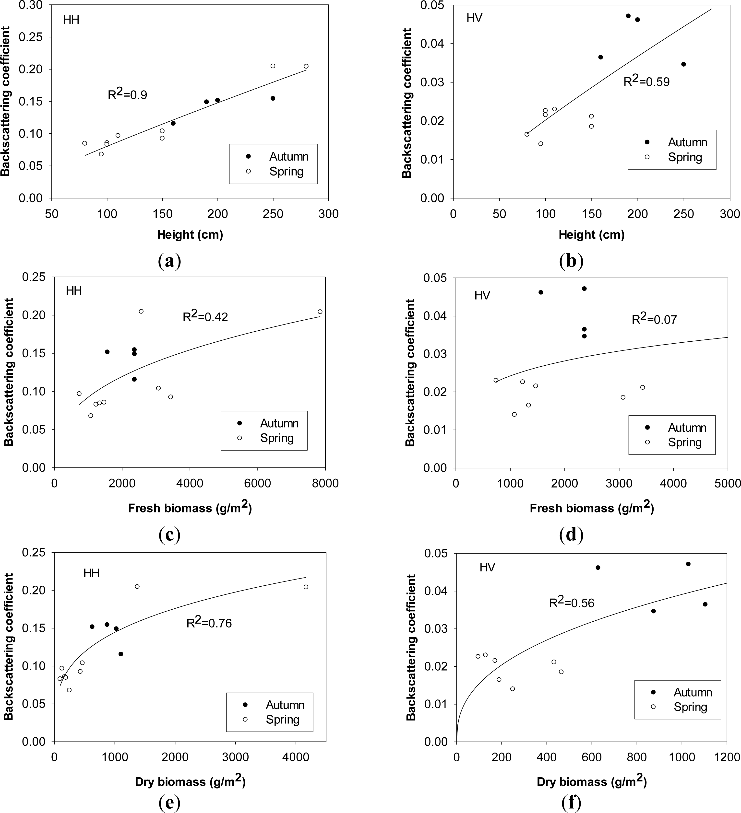
Plant height is one of the most important parameters used to determine the penetration depth of incident microwave signals and the contribution of canopy layer to radar backscattering coefficients. Both HH- and HV-polarized backscattering coefficients increases significantly, as broad leaves developed in vertical and horizontal directions to over 50 cm and plants height increases to over 200 cm during the maturity stage. Plant height is heavily correlated with radar backscattering coefficients in HH and HV polarizations, which suggests that the effect of plant height on the variation of radar backscattering coefficients enhances canopy volume scattering. No evident saturation point exists, and both HH- and HV-polarized backscattering increase over 3.5 dB as plant height ranges between 50 cm and 280 cm. Variations of plant height were also observed to make significant effects on C-band HH- (RADARSAT) and VV- backscattering coefficients (ERS) of natural herbaceous wetlands and paddy rice fields [15,21,22,60]. A simple quadratic polynomial was used to quantify the dependence of radar backscatter on plant height of paddy rice with high significance. Unlike this study, both HH-polarized RADARSAT and VV-polarized ERS-1 radar backscatter reached their saturation levels at the plant height of about 80 cm [22,60]. A saturation point at 0.6 m plant height for the C-band and 0.7 m plant height for the L-band for aquatic vegetation was also observed for wild wetland grass in the Amazon floodplain. In this study, the coefficient of determination of radar backscattering coefficients against plant height is less in HV polarization (R2 = 0.59) than in HH polarization (R2 = 0.9) with the confidence level of 95%, which indicates that HH polarization is more sensitive to plant height of Phragmites communis Trin. with dominant vertical orientation (Figure 6a,c). Similar high dependency of HH-polarized radar backscattering on plant height was also observed at C-band [15] and L-band from wetlands species [45]. However, the dependence of VV-polarized ERS backscatter on above-water plant height (ground water depth) was slight, although radar backscatter still linearly decreased with the rise of ground water [21]. A similar poor dependence of radar backscatter on plant height was also observed in C-band HH polarization [45]. Therefore, the effect of plant height on radar backscatter is highly dependent on plant type, plant structure and ground water.
Dry biomass is also related to structural parameters, such as plant height and stem numbers. After the influence of vegetation moisture content is excluded, the sensitivity of radar backscattering coefficients to variations of dry biomass is evident, especially in HH polarization (R2 = 0.76 with the confidence level of 95%), during the early growing stage.
High effect of plant biomass on both HH- and VV-polarized C-band backscatter was also observed from paddy rice [22,60]. L-band radar backscattering was more sensitive than C-band (both in HH polarization) to above-ground or above-water fresh/dry biomass for wild wetland grass due to the deeper penetration ability of L-band microwave signal, and their combination can improve the saturation level of radar backscatter [15]. However, in this study, ASAR backscattering coefficients do not change much when the dry biomass reaches the following values: 1300 g/m2 for HH polarization and 630 g/m2 for HV polarization, due to the attenuation of vegetation canopy layer to microwave signals. ASAR backscattering reaches saturated at the fresh biomass level of 2500 g/m2 in HH polarization. Similarly, saturation points of dry biomass were also observed for the C-band and L-band HH-polarized backscattering coefficients for Amazonian aquatic vegetation [15]. Although the samples are divided into two groups (spring and autumn), similar to plant height, dry biomass samples from these two groups do not show any difference, and their relationships with HH and HV backscattering coefficients keep constant (Figure 6b,d).
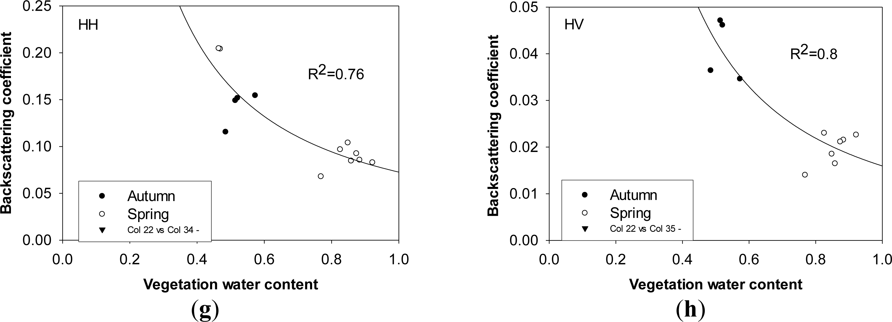
Generally, vegetation water content exerts a negative effect on radar backscattering coefficients in both polarizations, and it enhances the ability of attenuation in canopy layer rather than make a contribution to canopy volume scattering. Unlike the positive influence of plant water content on radar backscattering coefficients in HH polarization at the P-, L- and C-bands as observed for agriculture [61], it plays a negative role in radar mechanisms in HH and HV polarizations in this study. Although radar backscattering coefficients are highly dependent on plant water content (R2 = 0.76 for HH polarization, R2 = 0.8 for HV polarization, ρ < 0.05) when field samples are grouped together, the correlation between plant water content and dry biomass/height cannot be ignored, which is different in autumn from spring (Figure 6f,h).
Fresh biomass is composed of dry biomass and vegetation water content, but the latter two exert inverse effects on radar mechanisms according to above analysis. Therefore, the dependence of radar backscattering coefficients on fresh biomass is not distinct, especially in HV polarization. HH-backscattering coefficient roughly reaches saturation point at the fresh biomass level of 2500 g/m2, and HV is not sensitive to fresh biomass (R2 = 0.07, ρ < 0.05) (Figure 6e,g). Similarly, C-band ERS backscattering coefficients were also saturated at the biomass level of 1000 g/m2 for totoras and 2000 g/m2 for Puna bofedles in Andean wetlands [39]. The variation of above-ground/water biomass had a relatively little impact on the change in ERS backscatter when considering the variations in soil moisture and water level, and it was concluded to be due to the short canopy and low biomass level in the study sites [21]. However, unlike this study, high dependency of C-band HV- backscattering coefficients on the variation of fresh biomass existed for short crops (colza, alfalfa and wheat), but the sensitivity decreased for tall crops (corn, sunflower and sorghum) as observed by AIRSAR and SIR-C [61].
Although the empirical models quantifying the relationships of ASAR backscattering with vegetation parameters (plant height, fresh/dry biomass, and vegetation water content) of Phragmites communis is informative, the analysis results are heavily affected by the limited field collections. Any irregular measurements caused by environment conditions or anthropic factors will change the trend of the fitted curve. More field measurements covering the whole growing cycle should be further collected from this wetland community to increase its reliability.
5.4. The Relationships between Radar Backscatter and Vegetation Biophysical Parameters of Cares spp
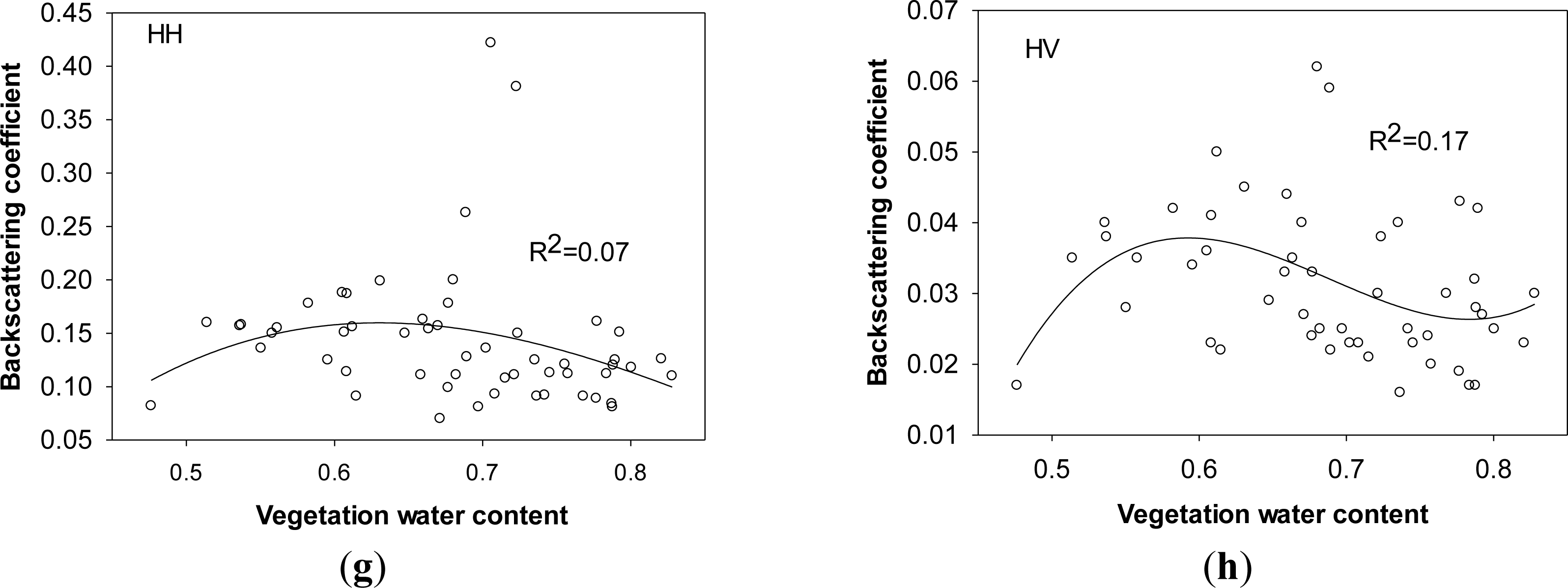
According to the simulation results from wetlands in southern Florida, the influence of soil moisture variability on ERS VV-backscatters with incident angle of 23° decreases with the increase of plants biomass, and no change occurred in VV-backscatters as soil moisture ranged between 0 and 1 cm3/cm3 at the biomass level of 1680 g/m2 [21]. In addition, the simulated L-band backscatter would not change much in HH and VV polarization as soil volumetric moisture content was higher than 0.4 cm3/cm3 [56]. In this study, the effects of soil moisture on C- band radiation with incident angle of over 33° are ignored in spring and autumn. Ground surface roughness data are not collected in field work, and in this study, only the relationships of canopy parameters with HH- and HV-backscattering coefficients are analyzed. A fitted cubic polynomial function between vegetation parameters and ASAR backscattering of Carex spp.is utilized:
HV polarization as a “depolarization” phenomenon caused by canopy leaves is more sensitive to vegetation parameters than HH polarization. However, due to the influence of environmental conditions (wind, dews, rain drops, and ground water), the effects of vegetation parameters of Carex spp., including plant height, fresh and dry biomass, and plant water content, on radar signals in both polarizations are not significant. As observed in Figure 7, HH and HV polarized backscatters does not increase much when above-ground plant height of Carex spp. is over 30 cm and fresh biomass is over 1300 g/m2. The saturation points of plant height and fresh biomass of Carex spp. are much lower than those of Phragmites communis as shown in previous section and other observed results [12,15,18,36]. The complicated backscattering mechanism from this wetland community needs be quantitatively interpreted by building physically based model.
6. Conclusions
C-band ENVISAT/ASAR fine mode alternating-polarization imager are utilized in Poyang Lake wetland of Jiangxi province, China, to investigate the temporal radar backscattering mechanism and to understand the relationships between radar backscattering coefficients and wetland biophysical characteristics. ASAR backscattering coefficients and mechanisms from two wetland communities with different canopy structure (Phragmites Trin. and Carex spp.) are analyzed with the change of canopy parameters and ground water conditions. Although the time series of ASAR data does not cover the whole growing cycle of wetland species, some particular development stages of these two wetland species were still monitored. For the purpose of mapping different wetlands in Poyang Lake region, C-band fine-mode ASAR imagery, especially in HH polarization mode, shows its potential to detect and map wetlands species colonizing those areas with different elevations.
In order to quantify the relationships of dual-polarized ASAR backscattering coefficients with vegetation biophysical parameters (plant height, aboveground fresh and dry biomass, and water content) of Poyang Lake wetland species, the sensitivity analysis of HH- and HV-backscattering to vegetation parameters is conducted for these two wetland species by using empirical regression models. The limitation of empirical relationships is that they are not directly transferable to other study sites, although enough field measurements were collected. The analysis indicates that C-band ASAR backscattering is very sensitive to the variation of vegetation parameters of Phragmites communis. It is possible to build physically based radiative transfer mode to retrieve vegetation biomass. However, as observed by ASAR backscattering in HH and HV polarization, C-band backscattering is not sensitive to the variations of vegetation parameters of Carex spp., due to the complicated influencing factors controlled by vegetation structural parameters. Compared with Phragmites communis, it will be more difficult to build physical model to retrieval vegetation biomass for this wetland community. More field measurements, including vegetation structural parameters (leaf number, leaf length, leaf width, stem height, stem diameter, leaf and stem dielectric constant, etc.) and ground surface roughness, need to be collected from these two species. Physically based model simulating ASAR backscattering process would be developed to quantify radar backscattering from different wetland part and further to invert canopy biomass and other biophysical parameters.
Acknowledgments
This work was supported by National Basic Surveying and Mapping Research Program—Automatic Classification with Multi-source Remote Sensing Data in Complex Vegetation Coverage Area(A1408), Basic Research Fund of Chinese Academy of Surveying and Mapping (7771404), Open Fund of the Key Laboratory of Geo-Informatics of National Administration of Surveying, Mapping and Geoinformation, CASM (777142104), National Key Technology Research and Development Program of the Ministry of Science and Technology of China (2012BAH28B01). We also would like to acknowledge every member of the Global Land Cover project team at CASM.
Author Contributions
Huiyong Sang had the original idea for the study and, with all co-authors carried the design. Jixian Zhang and Hui Lin were responsible for recruitment and follow-up of study participants. Liang Zhai was responsible for data cleaning and processing. Huiyong Sang also carried out the analyses and drafted the manuscript, which was revised by all authors. All authors read and approved the final manuscript.
Conflicts of Interest
The authors declare no conflict of interest.
References
- Nixon, S. Between Coastal Marshes and Coastal Waters—A Review of Twenty Years of Speculation and Research on the Role of Salt Marshes in Estuarine Productivity and Water Chemistry. In Estuarine and Wetland Processes; Hamilton, P., Macdonald, K., Eds.; Plenum Press: New York, NY, USA, 1980; pp. 437–525. [Google Scholar]
- Roulet, N.T. Peatlands, carbon storage, greenhouse gases, and the Kyoto Protocol: Prospects and significance for Canada. Wetlands 2000, 20, 605–615. [Google Scholar]
- Mitsch, J.W.; Goselink, J.G. Wetlands, 2nd ed; Van Nostrand Reinhold: New York, NY, USA, 1993. [Google Scholar]
- Barlett, K.B.; Harriss, R.C. Review and assessment of methane emissions from wetlands. Chemoshpere 1993, 26, 261–320. [Google Scholar]
- Cicerone, R.J.; Oremland, R.S. Biogeochemical aspects of atmospheric methane. Global Biogeochem. Cycle 1988, 2, 371–354. [Google Scholar]
- Matthews, E.; Fung, I. Methane emission from natural wetlands: Global distribution, area and environmental characteristics of sources. Global Biogeochem. Cycle 1987, 1, 61–86. [Google Scholar]
- Ormsby, J.P.; Blanchard, B.J.; Blanchard, A.J. Detection of lowland flooding using active microwave systems. Photogramm. Eng. Remote Sens 1985, 51, 317–328. [Google Scholar]
- Hess, L.L. Delineation of inundated area and vegetation along the Amazon floodplain with the SIR-C synthetic aperture radar. IEEE Trans. Geosci. Remote Sens 1995, 33, 896–904. [Google Scholar]
- Pope, K.O.; Rejmankova, E.; Paris, J.F.; Woodruff, R. Detecting seasonal flooding cycles in marshes of the Yucatan Peninsula with SIR-C polarimetric radar imagery. Remote Sens. Environ 1997, 59, 157–166. [Google Scholar]
- Alsdorf, D.E.; Smith, L.C.; Melack, J.M. Amazon floodplain water level changes measured with interferometric SIR-C radar. IEEE Trans. Geosci. Remote Sens 2001, 39, 423–431. [Google Scholar]
- Bourgeau-Chavez, L.L.; Kasischke, E.S.; Brunzell, S.M.; Mudd, J.P.; Smith, K.B.; Frick, A.L. Analysis of space-borne SAR data for wetland mapping in Virginia riparian ecosystems. Int. J. Remote Sens 2001, 22, 3665–3687. [Google Scholar]
- Kourgli, A.; Ouarzeddine, M.; Oukil, Y.; Belhadj-Aissa, A. Texture modelling for land cover classification of fully polarimetric SAR images. Int. J. Image Data Fusion 2012, 3, 129–148. [Google Scholar]
- Yu, J.; Yan, Q.; Zhang, Z.; Ke, H.; Zhao, Z.; Wang, W. Unsupervised classification of polarimetric synthetic aperture radar images using kernel fuzzy C-means clustering. Int. J. Image Data Fusion 2012, 3, 319–332. [Google Scholar]
- Frate, F.D.; Daniele Latini, D.; Chiara Pratola, C.; Palazzo, F. PCNN for automatic segmentation and information extraction from X-band SAR imagery. Int. J. Image Data Fusion 2013, 4, 75–88. [Google Scholar]
- Costa, M.P.F.; Niemann, O.; Novo, E.; Ahern, F. Biophysical properties and mapping of aquatic vegetation during the hydrological cycle of the Amazon floodplain using JERS-1 and Radarsat. Int. J. Remote Sens 2002, 23, 1401–1426. [Google Scholar]
- Freeman, A.; Chapman, B.; Siqueira, P. The JERS-1 Amazon multi-season mapping study (JAMMS): Science objectives and implications for future missions. Int. J. Remote Sens 2002, 23, 1447–1460. [Google Scholar]
- Costa, M.P.F. Use of SAR satellites for mapping zonation of vegetation communities in the Amazon floodplain. Int. J. Remote Sens 2004, 25, 1817–1835. [Google Scholar]
- Rosenqvist, A.; Forsberg, B.R.; Pimentel, T.; Rauste, Y.A.; Richey, J.E. The use of spaceborne radar data to model inundation patterns and trace gas emissions in the central Amazon floodplain. Int. J. Remote Sens 2002, 23, 1303–1328. [Google Scholar]
- Wang, Y. Seasonal change in the extent of inundation on floodplains detected by JERS-1 synthetic aperture radar data. Int. J. Remote Sens 2004, 25, 2497–2508. [Google Scholar]
- Baghdadi, N.; Bernier, M.; Gauthier, R.; Neeson, I. Evaluation of C-band SAR data for wetlands mapping. Int. J. Remote Sens 2001, 22, 71–88. [Google Scholar]
- Kasischke, E.S.; Smith, K.B.; Bourgeau-Chavez, L.L.; Romanowicz, E.A.; Brunzell, S.; Richardson, C.J. Effects of seasonal hydrologic patterns in south Florida wetlands on radar backscatter measured from ERS-2 SAR imagery. Remote Sens. Environ 2003, 88, 423–441. [Google Scholar]
- Le Toan, T.; Ribbes, F.; Wang, L.F.; Floury, N.; Ding, K.H.; Kong, J.A.; Fujita, M.; Kurosu, T. Rice crop mapping and monitoring using ERS-1 data based on experiment and modeling results. IEEE Trans. Geosci. Remote Sens 1997, 35, 41–56. [Google Scholar]
- Nolan, M.; Fatland, D.R.; Hinzman, L.D. InSAR measurement of soil moisture. IEEE Trans. Geosci. Remote Sens 2003, 41, 2802–2813. [Google Scholar]
- Reschke, J.; Bartsch, A.; Schlaffer, S.; Schepaschenko, D. Capability of C-band SAR for operational wetlands monitoring at high latitudes. Remote Sens 2012, 4, 2923–2943. [Google Scholar]
- Arnesen, A.S.; Silva, T.S.F.; Hess, L.L.; Novo, E.M.L.M.; Rudorff, C.M.; Chapman, B.D.; McDonald, K.C. Monitoring flood extent in the lower Amazon river floodplain using AlOS/PALSAR ScanSAR images. Remote Sens. Environ 2013, 130, 51–61. [Google Scholar]
- Lopez-Sanchez, J.M.; Clouse, S.R.; Ballester-Berman, J.D. Rice phenology monitoring by means of SAR polarimetric X-band. IEEE Trans. Geosci. Remote Sens 2012, 50, 2695–2709. [Google Scholar]
- Sartori, L.R.; Imai, N.N.; Mura, J.C.; Novo, E.M.L.M.; Silva, T.S.F. Mapping macrophyte species in the Amazon floodplain wetlands using fully polarimetric ALOS/PALSAR data. IEEE Trans. Geosci. Remote Sens 2011, 49, 4717–4728. [Google Scholar]
- Wang, C.; Wu, J.; Zhang, Y.; Pan, G.; Qi, J.; Salas, W.A. Characterizing L-band scattering of paddy rice in southeast China with radiative. transfer model and multitemporal AlOS/PALSAR imagery. IEEE Trans. Geosci. Remote Sens 2009, 47, 988–998. [Google Scholar]
- Marti-Cardona, B.; Lopez-Martinez, C.; Dolz-Ripolles, J.; Bladè-Castellet, E. ASAR plolarimetric multi-incidence angle and multitemporal characterization of Donana wetlands for flood extent monitoring. Remote Sens. Environ 2010, 114, 2802–2815. [Google Scholar]
- Wetland Mapping in the West Silberian Lowlands with Envisat ASAR Global Mode. Available online: http://earth.esa.int/workshops/envisatsymposium/proceedings/sessions/4D3/462571ba.pdf (accessed on 12 May 2014).
- Lucas, R.M.; Mitchell, A.L.; Rosenqvist, A.; Proisy, C.; Melius, A.; Ticehurst, C. The potential of L-band SAR for quantifying mangrove characteristics and change: Case studies from the tropics. Acquat. Conserv.-Mar. Freshw. Ecosyst 2007, 17, 245–264. [Google Scholar]
- Bouvet, A.; Toan, T.L.; Lam-Dao, N. Monitoring of the rice cropping system in the Mekong delta using ENVISAT/ASAR dual polarization data. IEEE Trans. Geosci. Remote Sens 2009, 47, 517–526. [Google Scholar]
- Lin, H.; Chen, J.; Pei, Z.; Zhang, S.; Hu, X. Monitoring sugarcane growth using ENVISAT ASAR data. IEEE Trans. Geosci. Remote Sens 2009, 47, 2572–2580. [Google Scholar]
- Wang, X.; Ge, L.; Li, X. Pasture monitoring using SAR with COSMO-SkyMode, ENVISAT ASAR, and ALOS PALSAR in Otway, Australia. Remote Sens 2013, 5, 3611–3636. [Google Scholar]
- Santoro, M.; Cartus, O.; Fransson, J.E.S.; Shvidenko, A.; McCallum, I.; Hall, R.J.; Beaudoin, A.; Beer, C.; Schmullius, C. Estimated of forest growing stock volume for Sweden, Central Siberia, and Quebec using Envisat advanced synthetic aperture radar backscatter data. Remote Sens 2013, 5, 4503–4532. [Google Scholar]
- Wijaya, A.; Marpu, P.R.; Gloaguen, R. Discrimination of peatlands in tropical swamp forests using dual-polarimetric SAR and Landsat. ETM data. Int. J. Image Data Fusion 2010, 1, 257–270. [Google Scholar]
- Kasischke, E.S.; BourgeauChavez, L.L. Monitoring South Florida wetlands using ERS-1 SAR imagery. Photogramm. Eng. Remote Sens 1997, 63, 281–291. [Google Scholar]
- Dobson, M.C.; Ulaby, F.T.; Pierce, L.E. Land-cover classification and estimation of terrain attributes using synthetic-aperture radar. Remote Sens. Environ 1995, 51, 199–214. [Google Scholar]
- Moreau, S.; Le Toan, T. Biomass quantification of Andean wetland forages using ERS satellite SAR data for optimizing livestock management. Remote Sens. Environ 2003, 84, 477–492. [Google Scholar]
- Chen, J.; Lin, H.; Liu, A.; Shao, Y.; Yang, L. A semi-empirical backscattering model for estimation of leaf area index (LAI) of rice in southern China. Int. J. Remote Sens 2006, 27, 5417–5425. [Google Scholar]
- Baghdadi, N.; Boyer, N.; Todoroff, T.; Hajj, M.E.; Bégué, A. Potential of SAR sensors TerraSAR-X, ASAR/ENVISAT and PALSAR/ALOS for monitoring sugarcane crops on Reunion Island. Remote Sens. Environ 2009, 113, 1724–1738. [Google Scholar]
- Englhart, S.; Keuck, V.; Siegert, F. Aboveground biomass retrieval in tropical forests—The potential of combined X- and L-band SAR data use. Remote Sens. Environ 2011, 115, 1260–1271. [Google Scholar]
- Sandberg, G.; Ulander, L.M.H.; Fransson, J.E.S.; Holmgren, J.; Le Toan, T. L- and P-band backscatter intensity for biomass retrieval in hemiboreal forest. Remote Sens. Environ 2011, 115, 2874–2886. [Google Scholar]
- Oh, Y.; Hong, S.; Kim, Y.; Hong, J.; Kim, Y. Polarimetric backscattering coefficients of flooded rice fields at L- and C-bands: Measurements, modeling, and data analysis. IEEE Trans. Geosci. Remote Sens 2009, 47, 2714–2721. [Google Scholar]
- Novo, E.M.L.M.; Costa, M.P.F.; Mantovani, J.E. Lima., I.B.T. Relationship between macrophyte stand variables and radar backscatter at L and C band, Tucurui reservoir, Brazil. Int. J. Remote Sens 2002, 23, 1241–1260. [Google Scholar]
- Salas, W.; Boles, S.; Li, C.; Yeluripati, J.B.; Xiao, X.; Frolking, S; Green, P. Mapping and modelling of greenhouse gas emissions from rice paddies with satellite radar observations and the DNDC biogeochemical model. Aquatic conservation: Marine and freshwater ecosystems. 2007, 17. [Google Scholar] [CrossRef]
- Wang, Y.; Laura, L.; Hess, L.L.; Filoso, S.; Melack, J.M. Understanding the radar backscattering from flooded and nonflooded Amazonian forests: Results from canopy backscatter modeling. Remote Sens. Environ 1995, 54, 324–332. [Google Scholar]
- Silva, T.S.F.; Costa, M.P.F.; Melack, J.M. Spatial and temporal variability of macrophyte cover and productivity in the eastern Amazon floodplain: A remote sensing approach. Remote Sens. Environ 2010, 114, 1998–2010. [Google Scholar]
- Zhu, H.; Zhang, B. Poyang Lake; The University of Science and Technology of China Press: Hefei, China, 1997. (in Chinese) [Google Scholar]
- Liu, X.; Ye, J. Jiangxi Wetlands, 1st ed; Chinese Forestry Publishing Company: Beijing, China, 2000. (in Chinese) [Google Scholar]
- Wang, X.; Fan, Z.; Cui, L.; Yan, B.; Tan, H. Wetland Ecosystem Assessment of Poyang Lake; Science Publishing Company: Beijing, China, 2004. (in Chinese) [Google Scholar]
- Cheng, P. High-accuracy, low-cost SAR data correction—Geometric correction of ASAR data without ground control points. Photogram. Eng. Remote Sens 2006, 72, 6–8. [Google Scholar]
- Frost, V.S.; Josephine Abbott, S.; Shanmugan, K.S.; Holtzman, J. A model for radar images and its application to adaptive digital filtering of multiplicative noise. IEEE Trans. Pattern Anal. Mach. Intell 1982, PAMI-4, 157–166. [Google Scholar]
- Absolute Calibration of ASAR Level 1 Products Generated with PF-ASAR. Available online: http://envisat.esa.int/includes/resources/dsp_DocDetailsPopUp.cfm?fobjectid=4503 (accessed on 7 October 2004).
- Derivation of the Backscattering Coefficient Sigma-Nought in ESA ERS SAR PRI Products. Available online: http://earth.esa.int/ers/sysutil/ESC2.html (accessed on 7 May 2014).
- Ulaby, F.T.; Moore, R.K.; Fung, A.K. Radar Remote Sensing and Surface Scattering and Emission Theory; ARTECH House: Dedham, MA, USA, 1982. [Google Scholar]
- Shi, J.C.; Wang, J.; Hsu, A.Y.; O’Neill, P.E.; Engman, E.T. Estimation of bare surface soil moisture and surface roughness parameter using L-band SAR image data. IEEE Trans. Geosci. Remote Sens 1997, 35, 1254–1266. [Google Scholar]
- Dobson, M.C.; Ulaby, F.T.; Pierce, L.E.; Sharik, T.L.; Bergen, K.M.; Kellndorfer, J.; Kendra, J.R.; Li, E.; Lin, Y.C.; Nashashibi, A. Estimation of forest biophysical characteristics in Northern Michigan with SIR-C/X-SAR. IEEE Trans. Geosci. Remote Sens 1995, 33, 877–895. [Google Scholar]
- Wang, Y.; Kasischke, E.S.; Melack, J.M.; Davis, F.W.; Christensen, N.L. The effects of changes in loblolly pine biomass and soil moisture on ERS-1 SAR backscatter. Remote Sens. Environ 1994, 49, 25–31. [Google Scholar]
- Ribbes, F.; Le Toan, T. Rice field mapping and monitoring with RADARSAT data. Int. J. Remote Sens 1999, 20, 745–765. [Google Scholar]
- Ferrazzoli, P.; Paloscia, S.; Pampaloni, P.; Schiavon, G. The potential of multifrequency polarimetric SAR in assessing agricultural and arboreous biomass. IEEE Trans. Geosci. Remote Sens 1997, 35, 5–17. [Google Scholar]


| Date | Field Data of Phragmites Communis | Field Data of Carex spp. | ||||
|---|---|---|---|---|---|---|
| Soil Moisture (g/cm3) | Coverage (%) | Sampling Number | Soil Moisture (g/cm3) | Coverage (%) | Sampling Number | |
| 28 March | N/A | N/A | 20–90 | 9 | ||
| 15 April | 0.55 | 10 | 3 | 0.7–1 | 50–100 | 9 |
| 20 April | 0.37 | 20 | 4 | 0.7–1 | 60–100 | 9 |
| 25 May | 0.9 | 90 | 2 | flooded | 70 | 4 |
| 19 September | flooded | 15 | 2 | flooded | 0 | 0 |
| 18 October | 0.22 | 80 | 2 | Partly flooded | 20–60 | 4 |
| 26 October | 0.29 | 75 | 3 | Partly flooded | 50–90 | 9 |
| 19 November | N/A | Partly flooded | 90 | 4 | ||
| 28 November | 0.3 | 70 | 1 | 0.75 | 50–80 | 11 |
| 29 December | 0.57 | 5 | 1 | 0.6 | 30–70 | 9 |
| ASAR Data | Weather Conditions | ||||
|---|---|---|---|---|---|
| Dates | Swath/Incident Angle | Polarization | Temperature (°C) | Precipitation (mm) | Relative Humidity (%) |
| 27 March | IS4/30° | HH/HV | 11.8 | 21 | 92.3 |
| 15 April | IS5/35° | HH/HV | 16.4 | 0 | 52.7 |
| 18 April | IS7/45° | HH/HV | 18.2 | 6.7 | 76.5 |
| 25 May | IS6/40° | HH/VV | 21.0 | 0 | 81.1 |
| 24 June | IS5/35° | HH/VV | 28.3 | 0 | 76.8 |
| 14 Augst | IS4/30° | HH | 28.1 | 6.4 | 80.5 |
| 18 Sepember | IS4/30° | HH/HV | 28.9 | 0 | 73.8 |
| 26 October | IS6/40° | HH/HV | 17.4 | 0 | 92.1 |
| 19 November | IS4/30° | HH/HV | 9.8 | 3 | 73.7 |
| 27 November | IS4/30° | HH/HV | 13.6 | 0 | 92.3 |
| Vegetation Parameters | Polarization | R2 | Model Coefficients | t Statistic | ρ |
|---|---|---|---|---|---|
| Height | HH | 0.9 | a = 0.0014 | 2.0164 | 0.0688 |
| b = 0.8790 | 9.3612 | <0.0001 | |||
| HV | 0.59 | a = 0.0004 | 0.7698 | 0.4611 | |
| b = 0.8595 | 3.3839 | 0.008 | |||
| Fresh biomass | HH | 0.42 | a = 0.0072 | 1.0087 | 0.3348 |
| b = 0.3695 | 2.9478 | 0.0133 | |||
| HV | 0.07 | a = 0.0054 | 0.4483 | 0.6645 | |
| b = 0.2174 | 0.7366 | 0.4801 | |||
| Dry biomass | HH | 0.76 | a = 0.0202 | 3.0093 | 0.0119 |
| b = 0.2852 | 5.9202 | 0.0001 | |||
| HV | 0.56 | a = 0.0024 | 1.2655 | 0.2375 | |
| b = 0.4042 | 3.2764 | 0.0096 | |||
| Water content | HH | 0.76 | a = 0.0727 | 7.7503 | <0.0001 |
| b = −1.1703 | −5.5661 | 0.0002 | |||
| HV | 0.8 | a = 0.0160 | 7.318 | <0.0001 | |
| b = −1.4189 | −5.8314 | 0.0002 |
© 2014 by the authors; licensee MDPI, Basel, Switzerland This article is an open access article distributed under the terms and conditions of the Creative Commons Attribution license (http://creativecommons.org/licenses/by/3.0/).
Share and Cite
Sang, H.; Zhang, J.; Lin, H.; Zhai, L. Multi-Polarization ASAR Backscattering from Herbaceous Wetlands in Poyang Lake Region, China. Remote Sens. 2014, 6, 4621-4646. https://0-doi-org.brum.beds.ac.uk/10.3390/rs6054621
Sang H, Zhang J, Lin H, Zhai L. Multi-Polarization ASAR Backscattering from Herbaceous Wetlands in Poyang Lake Region, China. Remote Sensing. 2014; 6(5):4621-4646. https://0-doi-org.brum.beds.ac.uk/10.3390/rs6054621
Chicago/Turabian StyleSang, Huiyong, Jixian Zhang, Hui Lin, and Liang Zhai. 2014. "Multi-Polarization ASAR Backscattering from Herbaceous Wetlands in Poyang Lake Region, China" Remote Sensing 6, no. 5: 4621-4646. https://0-doi-org.brum.beds.ac.uk/10.3390/rs6054621