Article

Human Land-Use Practices Lead to Global Long-Term Increases in Photosynthetic Capacity

1
Department of Biology, University of Maryland, College Park, MD 20742, USA
2
Biodiversity and Climate Research Center, Senckenberg Gesellschaft für Naturforschung, Senckenberganlage 25, D-60325 Frankfurt, Germany
3
Department of Biological Sciences, Goethe University, Max-von-Laue-Straße 9, D-60438 Frankfurt, Germany
4
Smithsonian Conservation Biology Institute, National Zoological Park, Front Royal, VA 22630, USA
5
Department of Ecological Modeling, Helmholtz Center for Environmental Research-UFZ, D-04318 Leipzig, Germany
6
Code 610.9, NASA/Goddard Space Flight Center, Greenbelt, MD 20771, USA
7
Department of Geographical Sciences, University of Maryland, College Park, MD 20771, USA
8
National Socio-Environmental Synthesis Center (SESYNC), 1 Park Place, Suite 300, Annapolis, MD 21401, USA
*
Author to whom correspondence should be addressed.
Remote Sens. 2014, 6(6), 5717-5731; https://0-doi-org.brum.beds.ac.uk/10.3390/rs6065717
Submission received: 31 December 2013 / Revised: 4 May 2014 / Accepted: 13 May 2014 / Published: 18 June 2014
(This article belongs to the Special Issue Monitoring Global Vegetation with AVHRR NDVI3g Data (1981-2011))

Abstract

:
Long-term trends in photosynthetic capacity measured with the satellite-derived Normalized Difference Vegetation Index (NDVI) are usually associated with climate change. Human impacts on the global land surface are typically not accounted for. Here, we provide the first global analysis quantifying the effect of the earth’s human footprint on NDVI trends. Globally, more than 20% of the variability in NDVI trends was explained by anthropogenic factors such as land use, nitrogen fertilization, and irrigation. Intensely used land classes, such as villages, showed the greatest rates of increase in NDVI, more than twice than those of forests. These findings reveal that factors beyond climate influence global long-term trends in NDVI and suggest that global climate change models and analyses of primary productivity should incorporate land use effects.

1. Introduction

Climate change research often focuses on long-term productivity trends in vegetation at regional [13] to continental and global scales [4,5]. A key variable in these studies of vegetation productivity is the satellite-derived Normalized Difference Vegetation Index (NDVI), that is either used directly as a measure of photosynthetic capacity [6], or serves as an input variable for climate change models predicting terrestrial net primary production (NPP [5,7,8]). On a global scale, these studies often ignore that NDVI may not be driven by climate alone. Because the majority of the Earth’s ice-free land surface has been altered by human action [912] and because these same areas account for ~90% of terrestrial net primary production [13], trends in NDVI may also be linked to human land-use practices, such as land conversion, irrigation, and nitrogen deposition. Although several regional and local analyses demonstrate significant impacts on NDVI trends from changes in human land-use practices [1416], global-scale analyses relating trends of NDVI to these direct anthropogenic effects have received little attention [5].
Here, we provide one of the first global analyses of direct anthropogenic effects on long-term trends in NDVI from 1981 to 2010 (however see [17] for an analysis that also include land use but on a different scale). First, we quantified variation in NDVI trends across “anthromes” (anthropogenic biomes, after [13]). Anthromes were introduced by Ellis and Ramankutty [13] and classify the earths land surface based on a combination of data on population density, land-use, and land cover [13]. They characterize land surface based on global patterns of sustained, direct human interaction with ecosystems. Comparisons of trends in NDVI among anthromes thus represent a useful probe of direct anthropogenic effects on long-term trends in NDVI. We also examined the effect of human-population density, as a surrogate for the degree of anthropogenic effects. Lastly we tested for specific mechanistic linkages that may underlie spatial variation in trends of NDVI among ecoregions and investigated effects of human land conversion (measured as percentage village, urban areas and croplands per ecoregion), nitrogen deposition, and irrigation.

2. Results and Discussion

Globally, anthromes with intensive land use (dense settlements, villages, and croplands) all had significant (p < 0.05) and steep increases in annual mean NDVI over a 29-year period compared to other anthromes. Forests exhibited marginally significant increases (β = 0.0006, p = 0.06), whereas we found no significant trends for wildlands or rangelands (Figure 1A,C,E,G,I,K). We emphasize that wildlands in the anthropogenic biomes classification used here [13] simply lump all land surfaces that are free or almost free of any human footprint. They thus comprise extremely varied ecosystems across the globe where some may show positive and other may show negative trends. Our statement only refers to the average across all these diverse ecosystems.
We also calculated robust linear regression Theil-Sen (TS) slope estimators for each spatial location in the global NDVI data (using the GIMMS3g NDVI data). Across all anthromes, the medians of the per-pixel TS estimators agreed closely with the slope estimates of the annual mean (compare slope estimates in Figure 1(left) with medians in Figure 1(right)). Based on the average NDVI value in the respective anthromes, the TS estimators showed that NDVI of villages changed the most over the 29 year study period (5.9% increase), followed by dense settlements (4.3%) and croplands (3.7%). With a 2.5% increase, global net NDVI of forests increased less than half as much as villages. Global net NDVI increases in wildlands and rangelands were close to zero.
We show that in years where global NDVI decreased, the global average NDVI of land types such as villages or croplands appear to have dampened minima compared to wildlands or forests (compare minima in Figure 1A,C,E,G,I,K). Variation induced by seasonal changes in NDVI, such as those associated with the interplay between human activities and monsoon dynamics [18], complicate interpretation of this pattern.
In our second analysis, we tested for the effect of human-population density, as a surrogate for the degree of anthropogenic effects, and found strong linkages between trends in NDVI and human population density. Here, we used ecoregions as spatial units [19]. Ecoregions are distinct with respect to natural communities and resident species and thus ideal to test for spatial variation in anthropogenic effects on NDVI. In ecoregions with low human population densities, NDVI trends were small and close to zero, whereas in ecoregions with high population densities, NDVI increased significantly over time (Figure 2). For example, densely populated ecoregions with an average population density of ~500 people/km2 showed an average increase of ~0.025 NDVI units over the 29 year study period (a 6% increase compared to the global mean). Except for Australia, average annual increases in NDVI were also greater in more densely populated ecoregions when data were analyzed at the continental scale. Europe, which has the greatest average population density across ecoregions, showed the strongest relationship between trends in NDVI and population density (Figure 3).
Lastly, we tested for specific mechanistic linkages that may underlie spatial variation in trends of NDVI among ecoregions. In particular, we tested for human land conversion (measured as percentage village, urban areas, and croplands per ecoregion), nitrogen deposition, and irrigation and found that all three of these factors had significant effects. The percentage converted lands per ecoregion, the percent irrigated area per ecoregion, and the amount of nitrogen deposition all were positively related to increasing trends of NDVI (Table 1). Together these three factors explained 21% of the variation in trends in NDVI.
These results were robust to several methodological concerns and alternative hypotheses. For example, analyses excluding the moist tropical biome yielded similar results, suggesting the uncertainty of remote sensing estimates in the moist tropics [20] did not drive our findings (Table 2). Results were also robust to the hypothesis that humans have settled preferentially in areas with high NDVI (alternatively, that areas with high NDVI had greater absolute increases in NDVI) because standardizing the per-pixel TS estimators by the mean NDVI did not significantly change model outcomes (Table 2). Finally, results were robust to the spatial unit of analyses, because substituting the biologically defined ecoregions with square grid cells of length 500 km also did not substantially change model outcomes (Table 2).
Ecoregions with the fastest increases in NDVI were predominately located in temperate Europe, the Mediterranean, the Sudano-Sahelian belt in Africa, western India, and northern China (Figure 4A). Ecoregions with the fastest decreases were predominately located in boreal forests of North America, as well as dry forests in South America (mostly Paraguay) and drylands of northeastern Australia. When comparing ecoregions with the fastest NDVI increases (the 5% of land surface with the fastest increases in NDVI, n = 73 ecoregions) against those showing the largest NDVI decreases (the 5% of land surface with the fastest decreases in NDVI, n = 38 ecoregions), we found that the ecoregions exhibiting the fastest NDVI increases had a greater average population density (median of 94 vs. 7 persons per km2, Figure 4), greater percentage of converted lands (88% vs. 9%, Figure 4B), greater percentage of irrigated lands (49% vs. 4%, Figure 4B), and greater deposition of nitrogen (573 vs. 209 mg N/m2/year, Figure 4B).
Ecoregions with the fastest changes in NDVI corresponded well with decreases and increases in NDVI shown in other global and regional studies [5,21]. Decreasing trends in NDVI have been reported for ecoregions with the fastest decreases, like the Dry Chaco region in South America [14], northeastern Australia [22], and boreal Canada and Alaska [23,24]. Likewise, increasing trends in NDVI have been reported for ecoregions with the fastest increases across Europe [25,26], northern China [27], central India [2], and the Sudano-Sahelian belt in Africa [28,29].
Although trends in NDVI in some of these ecoregions, especially those with negative trends in remote areas like boreal Canada and Alaska or northeastern Australia, have been predominately attributed to climatic effects [2224], there is growing evidence for direct anthropogenic effects in almost all regions with significant human populations. For example, increasing trends in NDVI in India and northern China have been related to increasing rates of fertilization and irrigation [2,28]. Likewise, while previous studies have chiefly related the Sahelian greening trend to climate, e.g., [7], new investigations point to land conversion to croplands as one of the main causes for changes in NDVI [29]. In Europe, nitrogen deposition may be one of the main drivers of carbon sequestration in forests and—together with reforestation and climate changes—may well explain the large increases in NDVI observed across the continent [25,26,30]. We explain 35% of the variability in trends in NDVI by population density alone (Figure 3D), supporting the hypothesis that anthropogenic drivers are contributing to NDVI increases in Europe. There are also examples for direct anthropogenic effects in ecoregions with rapidly decreasing NDVI. Results of a recent study on deforestation undertaken by the UN-FAO [31] show that forest loss in South America accounts for more than 50% of the global forest area loss in the past two decades. One region particularly affected is the Dry Chaco in Paraguay, a region with rapid land conversion from forest to soybean plantation [32], identified by our analyses as an extremum for decreasing NDVI.

3. Experimental Section

3.1. NDVI Data and Pre-Processing

We used NDVI data from the Advanced Very High Resolution Radiometer (AVHRR) instrument developed into the GIMMS3g dataset (Global Inventory Modeling and Mapping Studies) [33,34]. Previous versions of the GIMMS data set have been used extensively for testing temporal trend in NDVI [35], have been tested against ground controls points [36] and are thought to be the best long term data set for analyzing long term trends in vegetation dynamics [37]. The current GIMMS3g dataset represents an improvement over previous AVHRR NDVI data sets because it was coprocessed with SeaWiFS and MODIS Terra data [20]. The SeaWiFS and MODIS instruments have spectral bands specifically designed for vegetation monitoring, better atmospheric correction algorithms, reduced geometric distortions, and improved radiometric sensitivity [38]. MODIS NDVI has been collected over the past 13 years from the Terra platform and the past 11 years from MODIS on the Aqua platform. For the respective MODIS overlap periods, the per-pixel trends in NDVI from GIMMS3g agree well with those from Terra and Aqua MODIS, except in the moist tropics, which are difficult for remote sensing due to humidity and cloud cover [20]. MODIS Terra and Aqua NDVI data do not compare well for the tropics either. Using the longer-term GIMMS3g dataset, we conducted the analyses discussed below twice, once with all terrestrial pixels and once excluding the moist tropics. Since our analyses used yearly means (see below) and the studies cited above did not compare yearly means of NDVI between MODIS and GIMMS3g, we performed additional analyses comparing annual means between MODIS terra and Aqua, and the GIMMS3g data set. We sampled 34 1-degree areas across the globe and found a high linear correlation between the MODIS and GIMMS data sets. A Gaussian mixed model between annual means of MODIS Terra and GIMMS3g accounting for sampling area with a random effect showed very close relationships between both data sets (β = 0.74, t = 24.57, N = 298, coefficient det. = 0.99) as did the same comparison with MODIS Aqua (β = 0.75, t = 25.79, N = 247, coefficient det. = 0.99). If the data was standardized by the mean NDVI across years of each area to make areas more comparable, the relationship was still strong. MODIS Terra vs. GIMMS3g: (β = 0.68, t = 21.25, N = 298, coefficient det. = 0.65) and MODIS Aqua vs. GIMMS3g: (β = 0.69, t = 22.62, N = 247, coefficient det. = 0.65).
The GIMMS3g dataset of bi-monthly NDVI composites provides global coverage at a spatial resolution of 8 km × 8 km. For our analyses, we used the 672 composites for the 29 year period 1982–2010. We rescaled the data to the original floating-point NDVI scaling of −1 to 1, we identified and removed falsely included water pixels with a correction layer based on vector layers of continental coastline, lakes and reservoirs [39], and we applied a minimum threshold that set all pixels with NDVI values less than 0.05 to 0.05. NDVI values below 0.05 indicate non-vegetated areas like bare soil, water, snow, and ice. This 0.05 threshold is based on an analysis of stable pixels in the Sahara Desert that had an average NDVI of 0.094 and has been used previously in studies examining trends in NDVI [40].

3.2. Trend Analysis & Anthropogenic Effects

We estimated linear trends of annual means of NDVI for the 29 point time series from 1982 to 2010 for each spatial location in the data set (n = 1,975,140 pixels) using the Theil–Sen (TS) median estimator (function mblm in package mblm in R). The TS estimator represents a robust linear regression method that calculates the median slope among all pairs of observations. Commonly used for studies in vegetation trends based on NDVI time-series [20,41,42], the TS estimator is relatively insensitive to outliers and is accurate even for skewed and heteroscedastic data.
To relate these estimates to anthropogenic effects we performed three different analyses. First, we evaluated trends in NDVI for each of the six groups of anthropogenic biomes identified by Ellis and Ramankutti [13]; wildlands, rangelands, forests, croplands, villages, and dense settlements. We calculated histograms and medians for the TS estimators for each group of anthropogenic biomes and the global trend for each group based on the yearly average of NDVI for all pixels of a group using generalized least squares (GLS). We incorporated the temporal correlation structure with a 1st order autoregressive moving average. For all GLS analyses, we calculated the coefficient of determination based on the improvement of the log-likelihood from the fitted null model (intercept only) to the full fitted model (function r.squaredLR in R package MuMIn, [43]).
Our second and third analyses were carried out on the scale of ecoregions. We used the World Wildlife Fund’s classification scheme, which distinguishes ecoregions [19] that are distinct with respect to natural communities and resident species. We first tested whether human-population density, as a surrogate for the degree of anthropogenic effects, was related to NDVI trends. We estimated human population density for each ecoregion as the mean of the 1990 and 2010 population estimates [44]. We next tested for the effects of land conversion, nitrogen deposition, and irrigation on NDVI trends by performing multiple regressions that included these factors as predictors. As a proxy for converted lands, we used the percent area covered by dense settlements, villages, and croplands per ecoregion [13]. For nitrogen deposition we used the mean nitrogen deposition per ecoregion in 1993 ([45], an average from the 1980s to the 2010s would have been preferable but was not available). For irrigation we calculated the percentage of irrigated area per ecoregion based on the UN-FAO irrigation map [46].
For both analyses we used the ecoregional means of the per-pixel TS estimators as the response variable. We used GLS accounting for spatial autocorrelation with an exponential spatial correlation function and accounting for differences in sizes of ecoregions using the inverse of ecoregion size as a weight in the variance function. For the multiple regression, we tested predictors for collinearity and used a cutoff correlation coefficient of 0.7 [47].
For robustness, we first repeated the analyses excluding all pixels located in the moist tropical broadleaf biome, because of unresolved and ongoing debates about the validity of remote sensing estimates in moist tropical regions [20,48] and the poor agreement between (1) GIMMS3g and MODIS Terra NDVI and (2) MODIS Terra and Aqua NDVI data in the moist tropics found by Fensholt and Proud [20]. Second, to ensure that our results do not stem from humans choosing areas with greater NDVI or from areas of greater NDVI exhibiting greater absolute increases of NDVI, we repeated our analyses by standardizing the per-pixel TS estimators by the mean NDVI value of each pixel. Third, even though ecoregions represent ecologically distinct units and as such are appropriate geographic units for examining the effects of covariates on trends in NDVI, we also repeated our analyses substituting squared grid cells of 500 km by 500 km for ecoregions. Lastly, to examine whether our results hold true also within continents and not just on the global scale, we performed the analyses for population density separately for each continent. Because some continents have only relatively few ecoregions, we did not perform the by-continent analyses for the multiple regression analyses.

4. Conclusions

In conclusion, our study provides one of the first global synopses quantifying the effect of the Earth’s human footprint on trends in photosynthetic capacity. Globally, more than 20% of the variability in NDVI trends can be associated with human land-use practices. Consequently, global climate change models and analyses of primary productivity should incorporate direct anthropogenic effects. Land use practices in densely populated areas, and other areas featuring major human impacts through land conversion, irrigation, and nitrogen deposition, may contribute more to global changes in photosynthetic capacity than previously anticipated.

Acknowledgments

WFF and TM were supported by NSF ABI award 1062411 and TM was supported by the Robert Bosch Foundation. This work was also supported by the National Socio-Environmental Synthesis Center (SESYNC) under funding received from the National Science Foundation DBI-1052875.

Conflicts of Interest

The authors declare no conflict of interest.
  • Author ContributionsThomas Mueller, Gunnar Dressler, Compton J. Tucker and William F. Fagan conceptualized the study, Thomas Mueller and Gunnar Dressler analyzed the data, and all authors contributed to the writing of the manuscript.

References

  1. Anyamba, A.C.; Tucker, J. Analysis of Sahelian vegetation dynamics using NOAA-AVHRR NDVI data from 1981–2003. J. Arid Environ 2007, 63, 596–614. [Google Scholar]
  2. Jeyaseelan, T.; Roy, P.S.; Young, S.S. Persistent changes in NDVI between 1982 and 2003 over India using AVHRR GIMMS (Global Inventory Modeling and Mapping Studies) data. Int. J. Remote Sens 2007, 28, 4927–4946. [Google Scholar]
  3. Olsson, L.; Eklundh, L.; Ardö, J. A recent greening of the Sahel—Trends, patterns and potential causes. J. Arid Environ 2005, 63, 556–566. [Google Scholar]
  4. Myneni, R.B.; Nemani, R.R.; Running, S.W. Estimation of global leaf area index and absorbed par using radiative transfer models. IEEE Trans. Geosci. Remote Sens 1997, 35, 1380–1393. [Google Scholar]
  5. Nemani, R.R.; Keeling, C.D.; Hashimoto, H.; Jolly, W.M.; Piper, S.C.; Tucker, C.J.; Myneni, R.B.; Running, S.W. Climate-driven increases in global terrestrial net primary production from 1982 to 1999. Science 2003, 300, 1560–1563. [Google Scholar]
  6. Tucker, C.J.; Sellers, P.J. Satellite remote-sensing of primary production. Int. J. Remote Sens 1986, 7, 1395–1416. [Google Scholar]
  7. Hickler, T.; Eklundh, L.; Seaquist, J.W.; Smith, B.; Ardo, J.; Olsson, L.; Sykes, M.T.; Sjostrom, M. Precipitation controls Sahel greening trend. Geophys. Res. Lett 2005, 32. [Google Scholar] [CrossRef]
  8. Cao, M.K.; Prince, S.D.; Small, J.; Goetz, S.J. Remotely sensed interannual variations and trends in terrestrial net primary productivity 1981–2000. Ecosystems 2004, 7, 233–242. [Google Scholar]
  9. Sanderson, E.W.; Jaiteh, M.; Levy, M.A.; Redford, K.H.; Wannebo, A.V.; Woolmer, G. The human footprint and the last of the wild. Bioscience 2002, 52, 891–904. [Google Scholar]
  10. Mittermeier, R.A.; Mittermeier, C.G.; Brooks, T.M.; Pilgrim, J.D.; Konstant, W.R.; da Fonseca, G.A.B.; Kormos, C. Wilderness and biodiversity conservation. Proc. Natl. Acad. Sci. USA 2003, 100, 10309–10313. [Google Scholar]
  11. Foley, J.A.; DeFries, R.; Asner, G.P.; Barford, C.; Bonan, G.; Carpenter, S.R.; Chapin, F.S.; Coe, M.T.; Daily, G.C.; Gibbs, H.K.; et al. Global consequences of land use. Science 2005, 309, 570–574. [Google Scholar]
  12. Hurtt, G.C.; Chini, L.P.; Frolking, S.; Betts, R.A.; Feddema, J.; Fischer, G.; Fisk, J.P.; Hibbard, K.; Houghton, R.A.; Janetos, A.; et al. Harmonization of land-use scenarios for the period 1500–2100: 600 years of global gridded annual land-use transitions, wood harvest, and resulting secondary lands. Clim. Chang 2011, 109, 117–161. [Google Scholar]
  13. Ellis, E.C.; Ramankutty, N. Putting people in the map: Anthropogenic biomes of the world. Front. Ecol. Environ 2008, 6, 439–447. [Google Scholar]
  14. Baldi, G.; Nosetto, M.D.; Aragon, R.; Aversa, F.; Paruelo, J.M.; Jobbagy, E.G. Long-term satellite NDVI data sets: Evaluating their ability to detect ecosystem functional changes in South America. Sensors 2008, 8, 5397–5425. [Google Scholar]
  15. Bradley, B.A.; Mustard, J.F. Comparison of phenology trends by land cover class: A case study in the Great Basin, USA. Glob. Chang. Biol 2008, 14, 334–346. [Google Scholar]
  16. Neigh, C.S.R.; Tucker, C.J.; Townshend, J.R.G. North American vegetation dynamics observed with multi-resolution satellite data. Remote Sens. Environ 2008, 112, 1749–1772. [Google Scholar]
  17. Eastman, J.R.; Sangermano, F.; Machado, E.A.; Rogan, J.; Anyamba, A. Global trends in seasonality of Normalized Difference Vegetation Index (NDVI), 1982–2011. Remote Sens 2013, 5, 4799–4818. [Google Scholar]
  18. Niyogi, D.; Kishtawal, C.; Tripathi, S.; Govindaraju, R.S. Observational evidence that agricultural intensification and land use change may be reducing the Indian summer monsoon rainfall. Water Resour. Res 2010. [Google Scholar] [CrossRef]
  19. Olson, D.M.; Dinerstein, E.; Wikramanayake, E.D.; Burgess, N.D.; Powell, G.V.N.; Underwood, E.C.; D’Amico, J.A.; Itoua, I.; Strand, H.E.; Morrison, J.C.; et al. Terrestrial ecoregions of the worlds: A new map of life on earth. Bioscience 2001, 51, 933–938. [Google Scholar]
  20. Fensholt, R.; Proud, S.R. Evaluation of earth observation based global long term vegetation trends—Comparing GIMMS and MODIS global NDVI time series. Remote Sens. Environ 2012, 119, 131–147. [Google Scholar]
  21. De Jong, R.; de Bruin, S.; de Wit, A.; Schaepman, M.E.; Dent, D.L. Analysis of monotonic greening and browning trends from global NDVI time-series. Remote Sens. Environ 2011, 115, 692–702. [Google Scholar] [Green Version]
  22. Donohue, R.J.; McVicar, T.R.; Roderick, M.L. Climate-related trends in Australian vegetation cover as inferred from satellite observations, 1981–2006. Glob. Chang. Biol 2009, 15, 1025–1039. [Google Scholar]
  23. Verbyla, D. Browning boreal forests of western North America. Environ. Res. Lett 2011, 6. [Google Scholar] [CrossRef]
  24. Beck, P.S.A.; Juday, G.P.; Alix, C.; Barber, V.A.; Winslow, S.E.; Sousa, E.E.; Heiser, P.; Herriges, J.D.; Goetz, S.J. Changes in forest productivity across Alaska consistent with biome shift. Ecol. Lett 2011, 14, 373–379. [Google Scholar]
  25. Julien, Y.; Sobrino, J.A.; Verhoef, W. Changes in land surface temperatures and NDVI values over Europe between 1982 and 1999. Remote Sens. Environ 2006, 103, 43–55. [Google Scholar]
  26. Stockli, R.; Vidale, P.L. European plant phenology and climate as seen in a 20-year AVHRR land-surface parameter dataset. Int. J. Remote Sens 2004, 25, 3303–3330. [Google Scholar]
  27. Piao, S.L.; Fang, J.Y.; Zhou, L.M.; Guo, Q.H.; Henderson, M.; Ji, W.; Li, Y.; Tao, S. Interannual variations of monthly and seasonal Normalized Difference Vegetation index (NDVI) in China from 1982 to 1999. J. Geophys. Res.: Atmos 2003. [Google Scholar] [CrossRef]
  28. Heumann, B.W.; Seaquist, J.W.; Eklundh, L.; Jonsson, P. AVHRR derived phenological change in the Sahel and Soudan, Africa, 1982–2005. Remote Sens. Environ 2007, 108, 385–392. [Google Scholar]
  29. Begue, A.; Vintrou, E.; Ruelland, D.; Claden, M.; Dessay, N. Can a 25-year trend in Soudano-Sahelian vegetation dynamics be interpreted in terms of land use change? A remote sensing approach. Glob. Environ. Chang 2011, 21, 413–420. [Google Scholar]
  30. De Vries, W.; Posch, M. Modelling the impact of nitrogen deposition, climate change and nutrient limitations on tree carbon sequestration in Europe for the period 1900–2050. Environ. Pollut 2011, 159, 2289–2299. [Google Scholar]
  31. The State of the World’s Forests; Food and Agriculture Organization of the United Nations: Rome, Italy, 2011.
  32. Clark, M.L.; Aide, T.M.; Grau, H.R.; Riner, G. A scalable approach to mapping annual land cover at 250 m using MODIS time series data: A case study in the Dry Chaco ecoregion of South America. Remote Sens. Environ 2010, 114, 2816–2832. [Google Scholar]
  33. Pinzon, J.E.; Tucker, C.J. A non-stationary 1981–2012 AVHRR NDVI3g time series. Remote Sens 2014. submitted. [Google Scholar]
  34. Tucker, C.J.; Pinzon, J.E.; Brown, M.E.; Slayback, D.A.; Pak, E.W.; Mahoney, R.; Vermote, E.F.; El Saleous, N. An extended AVHRR 8-km NDVI dataset compatible with MODIS and SPOT vegetation NDVI data. Int. J. Remote Sens 2005, 26, 4485–4498. [Google Scholar]
  35. Zhou, L.M.; Tucker, C.J.; Kaufmann, R.K.; Slayback, D.; Shabanov, N.V.; Myneni, R.B. Variations in northern vegetation activity inferred from satellite data of vegetation index during 1981 to 1999. J. Geophys. Res.: Atmos 2001, 106, 20069–20083. [Google Scholar]
  36. Sobrino, J.A.; Julien, Y. Global trends in NDVI-derived parameters obtained from GIMMS data. Int. J. Remote Sens 2011, 32, 4267–4279. [Google Scholar]
  37. Beck, H.E.; McVicar, T.R.; van Dijk, A.; Schellekens, J.; de Jeu, R.A.M.; Bruijnzeel, L.A. Global evaluation of four AVHRR-NDVI data sets: Intercomparison and assessment against Landsat imagery. Remote Sens. Environ 2011, 115, 2547–2563. [Google Scholar]
  38. Justice, C.O.; Townshend, J.R.G.; Vermote, E.F.; Masuoka, E.; Wolfe, R.E.; Saleous, N.; Roy, D.P.; Morisette, J.T. An overview of MODIS Land data processing and product status. Remote Sens. Environ 2002, 83, 3–15. [Google Scholar]
  39. Natural Earth Data Sets. Available online: http://www.naturalearthdata.com/ (accessed on 30 May 2014).
  40. Slayback, D.A.; Pinzon, J.E.; Los, S.O.; Tucker, C.J. Northern hemisphere photosynthetic trends 1982–99. Glob. Chang. Biol 2003, 9, 1–15. [Google Scholar]
  41. De Beurs, K.M.; Henebry, G.M. A statistical framework for the analysis of long image time series. Int. J. Remote Sens 2005, 26, 1551–1573. [Google Scholar]
  42. Alcaraz-Segura, D.; Chuvieco, E.; Epstein, H.E.; Kasischke, E.S.; Trishchenko, A. Debating the greening vs. Browning of the North American boreal forest: Differences between satellite datasets. Glob. Chang. Biol 2010, 16, 760–770. [Google Scholar]
  43. Nagelkerke, N.J.D. A note on a general definition of the coefficient of determination. Biometrika 1991, 78, 691–692. [Google Scholar]
  44. Socioeconomic Data and Applications Center, Center for International Earth Science Information Network (CIESIN), Columbia University and Centro Internacional de Agricultura Tropical. Gridded Population of the World, Version 3, SEDAC. 2005. Available online: http://sedac.ciesin.columbia.edu/gpw (accessed on 30 May 2014).
  45. Global Maps of Atmospheric Nitrogen Deposition, 1860, 1993 and 2050. Available online: http://daac.ornl.gov//CLIMATE/guides/global_N_deposition_maps.html (accessed on 30 May 2014).
  46. Global Map of Irrigation Areas. Available online: http://www.fao.org/nr/water/aquastat/irrigationmap/index10.stm (accessed on 30 May 2014).
  47. Dormann, C.F.; Elith, J.; Bacher, S.; Buchmann, C.; Carl, G.; Carré, G.; Marquéz, J.R.G.; Gruber, B.; Lafourcade, B.; Leitão, P.J.; et al. Collinearity: A review of methods to deal with it and a simulation study evaluating their performance. Ecography 2012, 36, 27–46. [Google Scholar]
  48. Saleska, S.R.; Didan, K.; Huete, A.R.; da Rocha, H.R. Amazon forests green-up during 2005 drought. Science 2007. [Google Scholar] [CrossRef]
Figure 1. Trends of NDVI for different groups of anthropogenic biomes (after [13]): Wildlands (A,B), Rangelands (C,D), Forested (E,F), Croplands (G,H), Villages (I,J) and Dense settlements (K,L). (Left): Annual mean NDVI and trends based on generalized least square models with an AR1 autocorrelation structure. β: coefficient of year, d: coefficient of determination, significance codes: * p < 0.05, ** p < 0.001, ns: not significant. (Right): Distributions of per-pixel Theil-Sen estimators, red line: median of distribution; black line indicates zero; als: area land surface of the globe.
Remotesensing 06 05717f1aRemotesensing 06 05717f1b
Figure 2. Annual change of NDVI of ecoregions, based on ecoregional means of per-pixel Theil-Sen estimators) vs. human population density. Circle diameters are proportional to the size (area) of each ecoregion. Red line indicates trend based on generalized least squares model with exponential spatial autocorrelation structure and accounting for differences in sizes of ecoregions in the variance function (β: 0.00032, p < 0.0001, Δ AIC: 105, coef. determination: 0.13). For corresponding analyses by continent, see Figure 3.
Remotesensing 06 05717f2
Figure 3. Annual change of NDVI of ecoregions (Africa (A), Asia (B), Australia (C), Europe (D), North America (E), South America (F), based on ecoregional means of per-pixel Theil-Sen estimators) vs. log10 of human population density. Circle diameters are proportional to the size (area) of each ecoregion. Red line indicates trend based on generalized least squares model with exponential spatial autocorrelation structure and accounting for differences in sizes of ecoregions in the variance function. β: coefficient of log10 of human population density, d: coefficient of determination, significance codes: *** p < 0.0001, ns: not significant.
Remotesensing 06 05717f3
Figure 4. (A) Trends in NDVI across the globe, 1981–2010. Ecoregional [19] extremes for NDVI increase (defined as the 5% of land surface with the fastest increases in NDVI, n = 73 ecoregions) are in red, whereas ecoregional extremes for NDVI decrease (defined as the 5% of land surface with the fastest decreases in NDVI, n = 38 ecoregions) are in blue; (B) Boxplots contrast the ecoregional extremes in A for increases (n = 73) and decreases (n = 38) in terms of NDVI trends, population density, percent converted lands [13], percent irrigated lands, and nitrogen deposition.
Remotesensing 06 05717f4
Table 1. Results from multiple regression analysis of the importance of possible drivers of trends in NDVI. Analyses were performed using ecoregional means of per-pixel TS estimators of trends in NDVI (n = 770, coefficient determination: 0.21, Δ AIC: 171, overall significance: <0.0001).
βp-Value
Intercept0.00017<0.0001
Converted lands (% area)0.00040<0.0001
Nitrogen (mg N/m2/year)0.000000250.0001
Irrigation (% area)0.000250.013
Table 2. Additional models relating trends in NDVI to (A) population density and (B) to nitrogen deposition, irrigation, and converted lands in order to ensure robustness of results against potential methodological concerns (see main text).
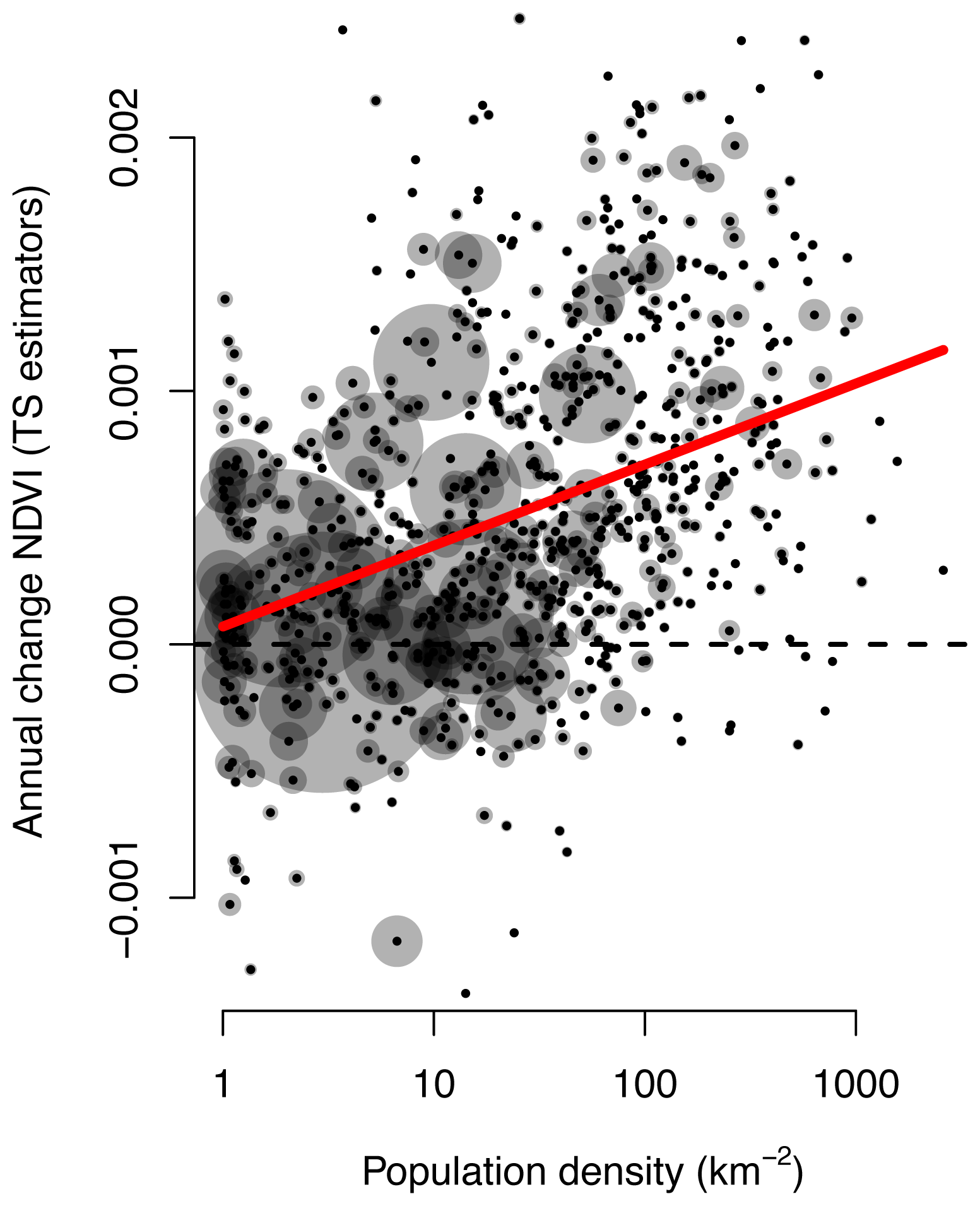
A. Models Relating Trends in NDVI to Population Density
Excluding the Moist Tropical Broadleaf Biome
βp-Value
Intercept−0.0000540.25
Log10 Population (m−2)0.00036<0.0001

Using Standardized TS Estimators
Coefficient of determination: 0.10, Δ AIC: 80, overall significance: <0.0001
βp-Value
Intercept0.0000430.68
Log10 Population (m−2)0.00069<0.0001

Using Fishnet as Spatial Unit
Coefficient of determination: 0.059, Δ AIC: 49, overall significance: <0.0001.
βp-Value
Intercept0.00024<0.0001
Log10 Population (m−2)0.00023<0.0001

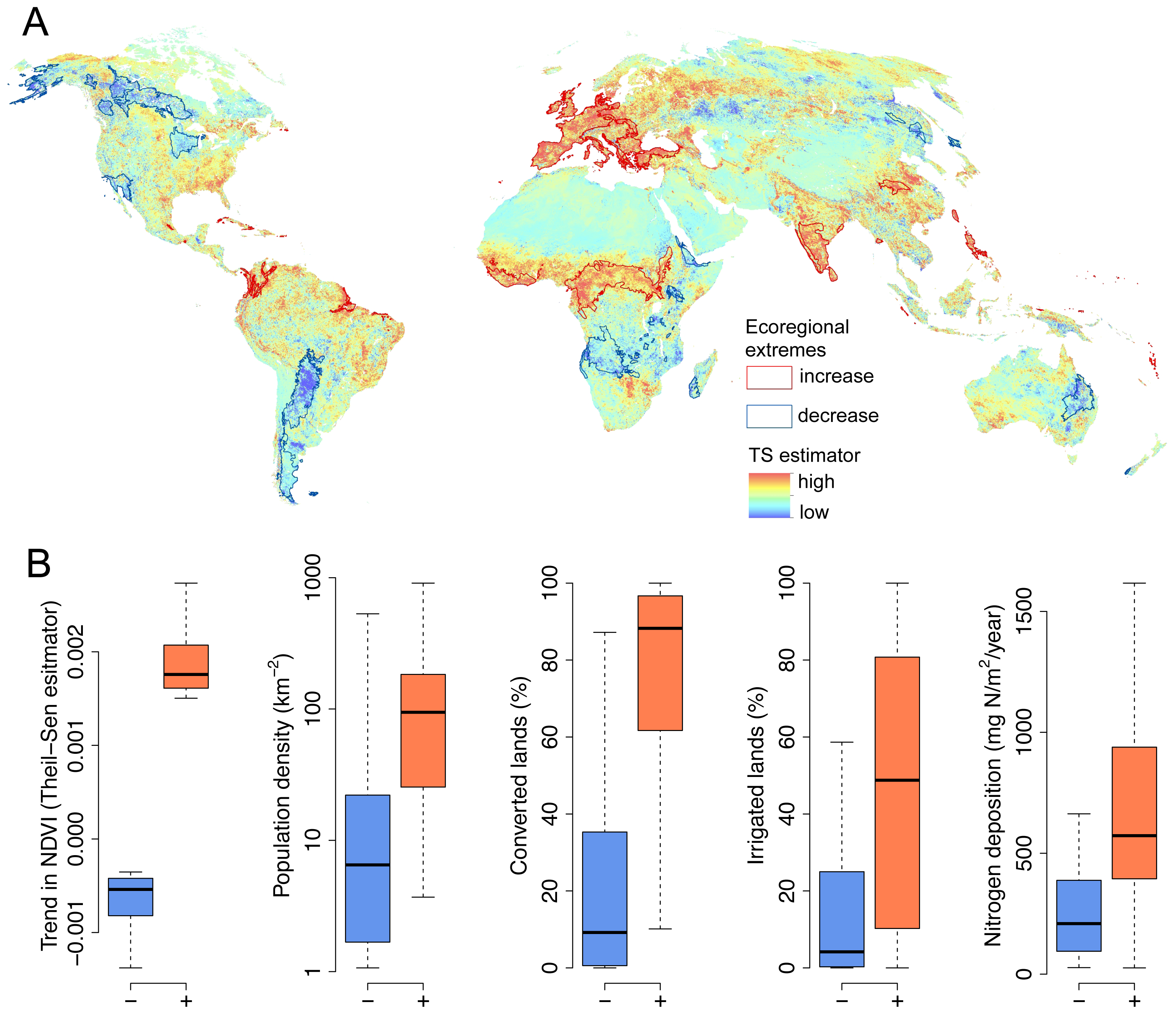
B. Models Relating Trends in NDVI to Nitrogen Deposition, Irrigation, and Converted Lands
Excluding the Moist Tropical Broadleaf Biome
Coefficient of determination: 0.26, Δ AIC: 164, overall significance: <0.0001.
βp-Value
Intercept0.0000680.044
Converted lands (% area)0.00046<0.0001
Nitrogen (mg N/m2/year)0.000000230.0022
Irrigation (% area)0.000350.0028

Using Standardized TS Estimators
Coefficient of determination: 0.15, Δ AIC: 122, overall significance: <0.0001.
βp-Value
Intercept0.000290.0002
Converted lands (% area)0.000530.024
Nitrogen (mg N/m2/year)0.000000430.0075
Irrigation (% area)0.00100.0001

Using Fishnet as Spatial Unit
Coefficient of determination: 0.11, Δ AIC: 88, overall significance: <0.0001
βp-Value
Intercept0.00022<0.0001
Converted lands (% area)0.000370.0003
Nitrogen (mg N/m2/year)0.000000150.020
Irrigation (% area)0.000310.0064

