Estimates of Aboveground Biomass from Texture Analysis of Landsat Imagery

Abstract

Maps of forest biomass are important tools for managing natural resources and reporting terrestrial carbon stocks. Using the San Juan National Forest in Southwest Colorado as a case study, we evaluate regional biomass maps created using physical variables, spectral vegetation indices, and image textural analysis on Landsat TM imagery. We investigate eight gray level co-occurrence matrix based texture measures (mean, variance, homogeneity, contrast, dissimilarity, entropy, second moment and correlation) on four window sizes (3 × 3, 5 × 5, 7 × 7, 9 × 9) at four offsets ([1,0], [1,1], [0,1], [1,−1]) on four Landsat TM bands (2, 3, 4, and 5). The map with the highest prediction quality was created using three texture metrics calculated from Landsat Band 2 on a 3 × 3 window and an offset of [0,1]: entropy, mean and correlation; and one physical variable: slope. The correlation of predicted versus observed biomass values for our texture-based biomass map is r = 0.86, the Root Mean Square Error is 45.6 Mg·ha⁻¹, and the Coefficient of Variation of the Root Mean Square Error is 0.31. We find that models including image texture variables are more strongly correlated with biomass than models using only physical and spectral variables. Additionally, we suggest that the use of texture appears to better capture the magnitude and direction of biomass change following disturbance compared to spectral approaches. The biomass mapping methods we present here are widely applicable throughout the US, as they are based on publically available datasets and utilize relatively simple analytical routines.

1. Introduction

Accurate spatial maps of forest biomass are necessary for managing forest resources, informing climate change modeling studies, and meeting national and international reporting requirements for greenhouse gas inventories [1,2]. Forest biomass maps are also necessary at the sub-national level for purposes such as completing the US Forest Service Climate Change Scorecard that necessitates annual estimates of carbon stocks and fluxes for each National Forest [3], and for quantifying changes in forest biomass on regional scales in response to disturbance. However, there are few spatially explicit regional and local biomass maps available, and as a consequence, relatively few resources available to determine how local biomass changes with disturbance. In this study we evaluate an alternative to traditional spectral analysis approaches to create local biomass maps.

There are two primary methods of mapping aboveground forest biomass. The first is an approach that assigns a biomass value, or a range of biomass values, to areas of land distinguished by characteristics such as vegetation type or land use. This approach, frequently referred to as “stratify and multiply”, uses ground-based measurements to determine biomass values, and spatial datasets to delineate mapping units. Although the stratify and multiply approach is relatively simple to implement, there are some limitations to this technique, namely the ambiguities present in land area classification, and the wide range of variability in aboveground biomass within a given land cover type [4].

The second common approach to mapping aboveground biomass employs a set of spatially continuous variables to predict biomass values at unobserved locations. In this direct mapping approach, a relationship is established between aboveground biomass and one or several spatially continuous variables, and these relationships are used to predict biomass across the population. The direct mapping approach takes advantage of a variety of geospatial variables, such as climate and topography, and information from remote sensing platforms. Many types of remotely sensed information can be used to aid in mapping biomass such as spectral information from remotely sensed imagery [5], backscattered energy from Synthetic Aperture Radar (SAR) [6,7], and Light Detection and Ranging (LiDAR) [8]. The two primary advantages to using a direct mapping approach are (1) the resulting map will more accurately depict variations in biomass across the landscape; and (2) changes to mapped forest biomass are easier to update [4].

There are also some limitations to the direct mapping techniques, particularly related to the use of remotely sensed information. One limitation is the mismatch of spatial scale between the area encompassed by a measurement plot and the area of a remotely sensed pixel. In the case of Landsat imagery, the area of a measurement plot only accounts for a small part of the area represented by a pixel and the plot measurement value may not accurately represent the aggregate value of biomass within that pixel. This disparity in spatial scale can introduce error into the resulting map. Secondly, direct mapping techniques that employ spectral band ratios, such as the Normalized Difference Vegetation Index (NDVI) and the Enhanced Vegetation Index (EVI), tend to under-predict forest biomass in regions of high biomass and multi-storied forest canopies where NDVI in particular can saturate [9]. SAR is a promising technique for biomass estimation, particularly when used in conjunction with methods that model forest biomass by empirically relating backscatter to ground-based biomass measurements, and interferometric SAR (InSAR) techniques that can estimate forest height [10]. However, SAR biomass estimation techniques also saturate in regions of dense forest canopy [7,10], and SAR data is only available on a limited bases. Finally, LiDAR provides a direct measure of forest canopy height [8,11], but its wide scale use is currently limited by the expense of acquiring LiDAR data at fine spatial scales. Until these data access limitations are resolved, other publically available remote sensing products will be required to create regional biomass maps.

Texture analysis is an image processing technique that may address some of the existing problems with vegetation index saturation and the data acquisition constrains related to mapping forest biomass at regional scales. Texture is a measure of variability in pixel values among neighboring pixels for a defined analysis window. A primary advantage of texture is that it can be calculated from optical data, among other types of raster data. The use of optical imagery in calculating texture is advantageous because there are several sources of publically available optical imagery, including Landsat, and, therefore, mapping biomass with image texture analysis is not subject to the constraints in obtaining data that are present for SAR or LiDAR. Furthermore, image texture has been used to aid in mapping forest biomass in dense tropical forests [12], and in some regions texture is a better predictor of biomass than spectral vegetation indices [13,14]. Because texture has been shown to be an effective method of mapping biomass in dense canopies, and can be calculated on widely available optical imagery, texture may be a useful technique for improving biomass maps at local and regional scales.

In this work we use a case study of San Juan National Forest in southwest Colorado to evaluate whether inclusion of image texture features can be used to improve the prediction quality of local scale biomass maps for use in land management and research. We evaluate the prediction quality of local scale biomass maps constructed with physical variables, spectral variables, and image texture metrics. Our methods include only publically available data. The wide range of vegetation types and the complex topography of this region make San Juan National Forest an ideal location to evaluate remote sensing based biomass mapping methods.

2. Materials and Methods

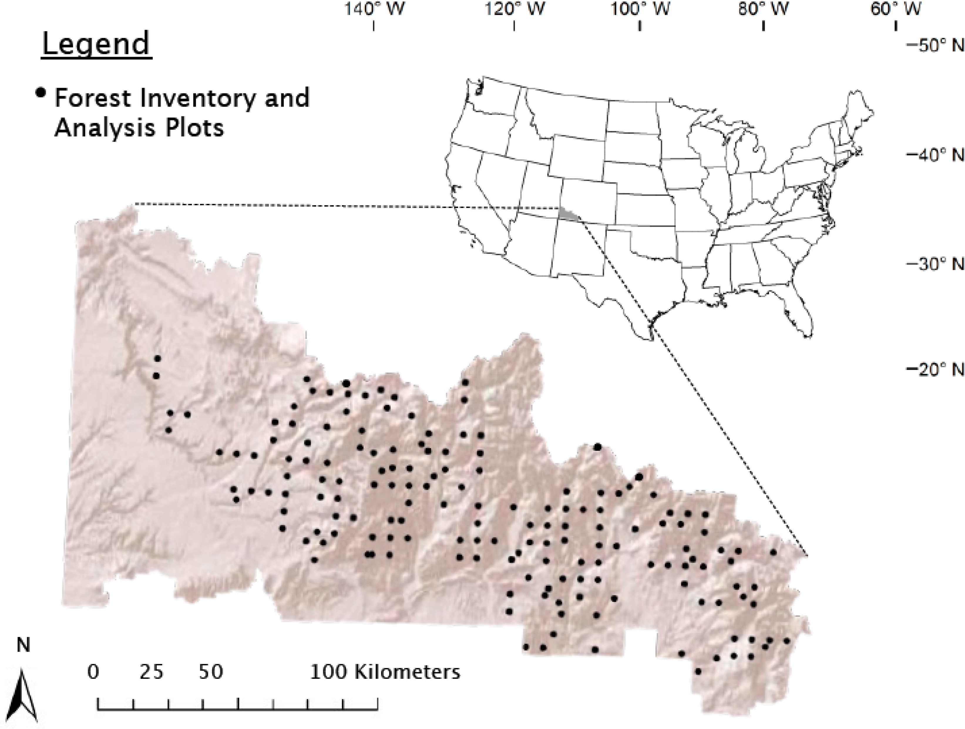
2.1. Study Area

The San Juan National Forest in southwest Colorado, USA is centered at 37°N and 108°W (Figure 1). This forest is roughly 7000 km² in area and ranges in elevation from 1500 m to 3800 m. Total annual average precipitation ranges from 400 mm in the lower elevations to over a meter (1150 mm) in the higher elevation forests [15]. Forests of this region contain Ponderosa Pine woodlands, Warm-Dry Mixed Conifer forests, Cool-Moist Mixed Conifer forests, and Spruce-Fir forests. San Juan National Forest is managed for recreation, timber production and wildfire fuel reduction, and is divided into stands that vary in stand age, treatment, and disturbance history. Landcover type for this region was determined from the Field Sampled Vegetation (FSVeg) database, an online inventory of information on trees, fuels, down woody material, surface cover, and understory vegetation, sampled and maintained by San Juan National Forest [16]. Only regions defined as forest were included in this study.

2.2. Field and Satellite Data

A total of 164 Forest Inventory and Analysis (FIA) Program plots from forested regions within San Juan National Forest (SJNF) were used for this study. The FIA Program consists of a system of ground-based forest inventory plots that are situated approximately one every 2400 ha throughout the coterminous United States, and are measured every 5 to 10 years [18]. FIA ground-based plot biomass data was obtained from the FIA online DataMart [19]. FIA plots consist of four 1/24 acre (168.7 m²) subplots in which live tree biomass is determined from measurements of tree dimensions. This biomass value is hereafter referred to as observed biomass. The observed biomass values for FIA plots within SJNF range from 2.1 to 490.2 Mg·ha⁻¹, with a mean biomass of 134.8 Mg·ha⁻¹. Although the exact location of FIA plots are not provided to the public, exact locations of the FIA plots within SJNF were obtained from the FIA program for the purposes of this study. All FIA plots used in this study were measured between 2002 and 2009. All plot locations were measured by FIA using the Global Positioning System (GPS), and have a horizontal accuracy of around 5 m [20].

Observed biomass values from eight independently sampled plots within or near forest stands clear-cut in the 1970’s were used to validate biomass predictions for clear-cut stands and adjacent untreated forest. Of these eight plots, five plots were located in untreated forest and three plots were located in stands clear-cut in the 1970s. Aboveground biomass measurements consisted of 50 m diameter circular plots (1963.49 m²) surveyed in 2012. Within each plot the diameter of every tree over 1.37 m tall was measured at 1.37 m to obtain a measure of diameter at breast height (DBH) for all trees within the plot. Aboveground live tree biomass was calculated from tree DBH using allometric equations [21,22]. Total observed aboveground live tree biomass was determined as the sum of all trees present within plot.

2.3. Landsat TM Image Analysis

For each FIA plot, spectral information was obtained for the corresponding geographic location from Landsat 5 TM imagery. Images from two adjacent Landsat TM paths were necessary to cover the entire spatial extent of the study area; the two images were acquired in June and July of 2011 (18 June; 21 July). The two scenes used in this study were selected because they are high-quality, cloud-free scenes acquired at similar dates and processed with Level 1T Standard Terrain Correction. All Landsat TM scenes were converted to top of atmosphere (TOA) reflectance using post-launch calibration coefficients [23], and an atmospheric correction was applied using Dark Subtraction Method [24]. A C-correction [25] was applied to correct for illumination differences due to sun-earth-sensor geometry across the variable topography of these two Landsat scenes using a 30-m resolution digital elevation model [26].

In this study, we evaluate the prediction quality of regional biomass maps constructed from physical variables, spectral variables, and image texture variables. The physical variables used included slope, aspect, and elevation calculated from regional digital elevation models [26], vegetation type determined from the SJNF FSVeg database, and precipitation obtained from the PRISM Climate Group [15]. The spectral information used included both the Normalized Difference Vegetation Index (NDVI) and the Enhanced Vegetation Index (EVI) calculated from Landsat TM imagery. Finally, image texture metrics were generated statistically using a Gray Level Co-occurrence Matrix (GLCM) computed from a relative displacement vector (d, θ) that describes the spatial distribution of grey level pairs separated by distance d in direction θ. Many textural metrics can be derived from the GLCM; we use the eight metrics of mean, variance, homogeneity, contrast, dissimilarity, entropy, second moment and correlation [27] as these eight have previously been used to good effect in mapping forest biomass in dense tropical forests [12,13,28]. In addition to d and θ, texture metrics are also dependent on the window size, or the number of pixels, used to calculate the GLCM. A small window size will identify fine-scale variations in pixel brightness while a large window will be sensitive to larger-scale variations. Therefore, a window that is too small may identify variations in pixel brightness that are irrelevant for the task at hand, whereas a window that is too large may overlook important variations in pixel brightness. For purposes of mapping forest biomass, the optimal window size was determined by the window size that had the strongest correlation between texture-predicted biomass and observed biomass. In order to determine the optimal window size for our study, all texture metrics were calculated on four Landsat TM bands (Bands 2–5) using four window sizes: 3 × 3, 5 × 5, 7 × 7, and 9 × 9 pixels. For each window size, texture was also calculated at four offsets, (θ), represented in Cartesian coordinates as [0,1], [1,1], [1,0], and [1,–1]. All GLCMs were constructed using a 64 gray level quantization; this value was chosen to reduce computational effort during GLCM construction, and to avoid creating sparse GLCMs [29].

2.4. Biomass Prediction

Physical variables, spectral vegetation indices, and texture metrics were used to predict aboveground forest biomass using feedforward neural networks built in Statistica12 (StatSoft, Inc., Tulsa, OK, USA). Neural networks are advantageous for this sort of modeling because they do not require any assumptions about the distribution and independence of input data. Our neural network model was constructed using FIA biomass values, and the corresponding physical, spectral and image texture information for that plot location. The observed biomass values from FIA plots were randomly divided into three groups: training, testing and validation data. Seventy percent of the plots were used as training data (116 plots), 15% as testing data (24 plots), and the remaining 15% as validation data (24 plots). Training data were used to build the network, testing data were used to refine the network as it was being built, and validation data were withheld from the training process and used to evaluate the map. The correlation between observed and predicted values for the training and testing groups was carefully monitored as the networks were being built in order to avoid over fitting; the correlation between the testing data and observed data was maintained below 0.7. The relative importance of each variable used in the neural network was evaluated using a global sensitivity analysis in Statistica. The sensitivity analysis is designed to test how the neural network predictions respond to changes in the input variable. The dataset is repeatedly submitted to the network, but each time one variable is replaced with its mean as calculated from the training data. The error in the resulting network is recorded, and the most important variables are identified as those that, when modified, result in the greatest increase in network error.

Forest biomass was predicted on a pixel-by-pixel basis for all forested regions of SJNF by using physical variables, spectral information and Landsat TM texture calculations as input to the neural network model. The model feature selection process is as follows: initial models were constructed using all combinations of physical, spectral, and texture variables. The model complexity was systematically reduced using the global sensitivity analysis to identify the most important variables in the model. We continued reducing the model complexity by removing the least important predictors as long as reductions continued to improve the model. Model quality was repeatedly evaluated using the four measures of error described below, and these measures were used to choose the final model.

2.5. Statistical Analyses

We used four statistical measures to evaluate model performance: Pearson’s Correlation (r),

$$\text{r}=\frac{\mathrm{\Sigma }\left(x_i-\overline{x}\right)\left(y_i-\overline{y}\right)}{\sqrt{\mathrm{\Sigma }{\left(x_i-\overline{x}\right)}^2}\sqrt{\mathrm{\Sigma }{\left(y_i-\overline{y}\right)}^2}}$$

(1)

where x is the observed value, x̄y is the average of the observed values, y is the predicted value and ȳ is the average of the predicted values; the Root Mean Square Error (RMSE):

$$\text{RMSE}=\sqrt{\frac{\mathrm{\Sigma }{\left(x_i-y_i\right)}^2}{n}}$$

(2)

where n is the number of observed values; the Coefficient of Variation of the Root Mean Square Error (CV-RMSE),

$$\text{CV}-\text{RMSE}=\frac{\mathit{RMSE}}{\overline{y}}$$

(3)

where RMSE is the root mean square error; and Akaike’s Information Criteria (AIC),

$$\text{AIC}=\text{n}\cdot \text{ln}\left(\frac{\text{SSE}}{\text{n}}\right)+2\text{k}$$

(4)

where SSE is the summed square error of the model and k is the number of model parameters. AIC is a relative measure of model quality for a given dataset and it provides a means for model selection based on both model fit and model parsimony. In other words, AIC values aid in identifying the model that provides the best description of the data using the smallest number of parameters. Higher quality models are identified by lower AIC values; generally AIC values that differ by >2 indicate that the model with the lower AIC is superior, whereas models with AIC values differing by <2 are similarly effective in describing the data [30].

Biomass prediction quality was also evaluated at fine spatial scales within two regions of the forest with a history of forest disturbance. Forest biomass predicted by the best performing texture-based map was compared to the biomass predicted by the best performing physical-spectral based map for two regions: a region with five forest stands clear-cut in the 1970s, and a region of forest burned by a wildfire in 2002. In each case the average predicted biomass within the disturbed stand was compared to the average predicted biomass in an adjacent undisturbed stand. Stand delineations were obtained from the SJNF FSVeg database.

3. Results

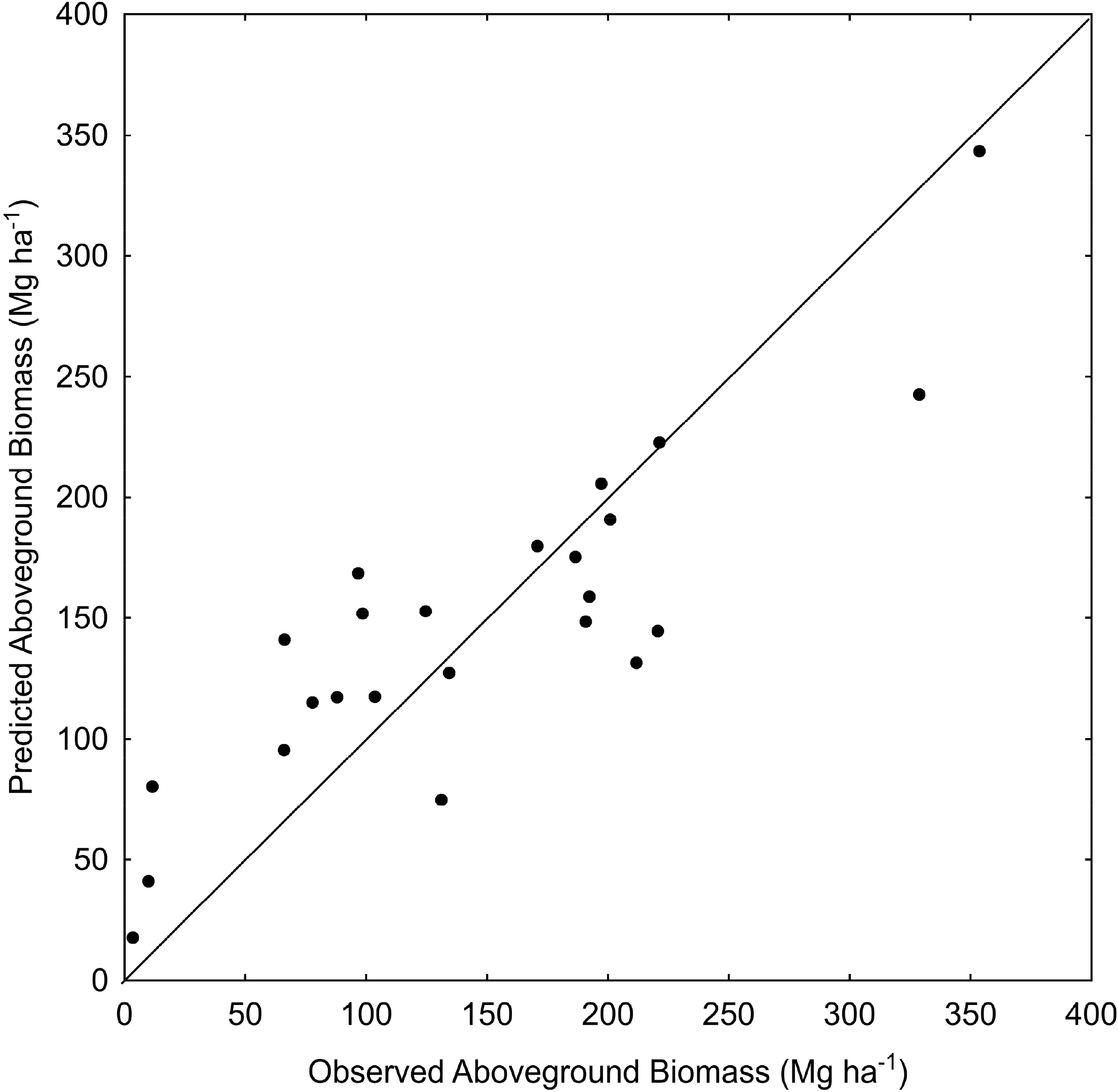
3.1. Biomass Prediction from Image Texture

Our final biomass map was constructed using the best performing neural network model constructed from the texture metrics of entropy, mean and correlation calculated from Landsat Band 2 on a 3 × 3 window and an offset of [0,1], and the physical variable slope (

Table 1. Correlation between predicted and observed biomass (r), Akaike’s Information Criteria (AIC), Root Mean Square Error (RMSE) and Coefficient of Variation Root Mean Square Error (CV-RMSE) for the five best performing neural network models constructed with texture metrics (top 5 rows), and the five best performing neural network models constructed without texture metrics (lower 5 rows). The architecture of each neural network is indicated in the form of input-hidden-output units. The Gray Level Co-occurrence Matrix (GLCM) texture metrics used in the highest preforming models were calculated on Band 2, on a 3 × 3 window at an (0,1) offset; they are: 1-mean, 2-variance, 3-homogeneity, 4-contrast, 5-dissimilarity, 6-entropy, 7-second moment, and 8-correlation.

Parameters	Network Architecture	r	AIC	RMSE	CV-RMSE
6, 1, 8, Slope	4-10-1	0.86	199.0	45.6	0.31
1, 6, 7, Slope, 8, 5	6-9-1	0.81	204.2	52.7	0.36
1, 8, Slope, 6, 5	5-6-1	0.84	207.4	51.9	0.36
1, Slope, 6	3-4-1	0.78	209.1	58.1	0.40
1, Slope, Aspect, 6, NDVI	5-9-1	0.79	211.7	56.4	0.39
Elevation, NDVI, Aspect, Slope	4-8-1	0.57	224.9	76.5	0.53
Elevation, Slope, Aspect	3-3-1	0.44	224.9	79.7	0.55
Elevation, Aspect, Slope, EVI, Precipitation	5-9-1	0.51	226.7	76.3	0.53
Elevation, Aspect, Slope, EVI	4-5-1	0.43	227.6	80.8	0.56
Vegetation Type, Aspect, Slope, Elevation	9-3-1	0.34	229.5	83.9	0.58

). The best performing network was determined as the model with the lowest RMSE and CV-RMSE, 45.6 Mg·ha⁻¹ and 0.31 respectively, the highest correlation between predicted and observed biomass values, 0.86, and the lowest AIC, 199.0 (Table 1; Figure 2). The AIC value of our best performing model differs from the next smallest AIC value of 204.2 by >5 indicating this model is preferable to the other models investigated (Table 1). Our biomass model predicts a wide range of aboveground biomass values across SJNF, with a maximum biomass value of 394 Mg·ha⁻¹. Generally the greatest biomass values were predicted in the high elevation regions and smaller biomass values in the lower elevations (Figure 3). A global sensitivity analysis was used to determine the importance of each variable in the context of this neural network. The texture variable mean contributed the most to this model, followed by correlation, the physical variable slope and the texture variable entropy. The relative importance of each variable is represented by the ratio of model error when the model is constructed excluding and including the variable in question. The relative sensitivities of mean, correlation, slope and entropy are 3.7, 1.8, 1.5, and 1.3, respectively.

Models including texture metrics performed better than those constructed with only physical variables (slope, aspect, elevation, precipitation and vegetation type) and spectral variables (NDVI and EVI; Table 1). The best-performing model constructed without any texture information was produced by a network including slope, aspect, elevation and NDVI (Table 1), and had a lower correlation, higher error and higher AIC than models including texture.

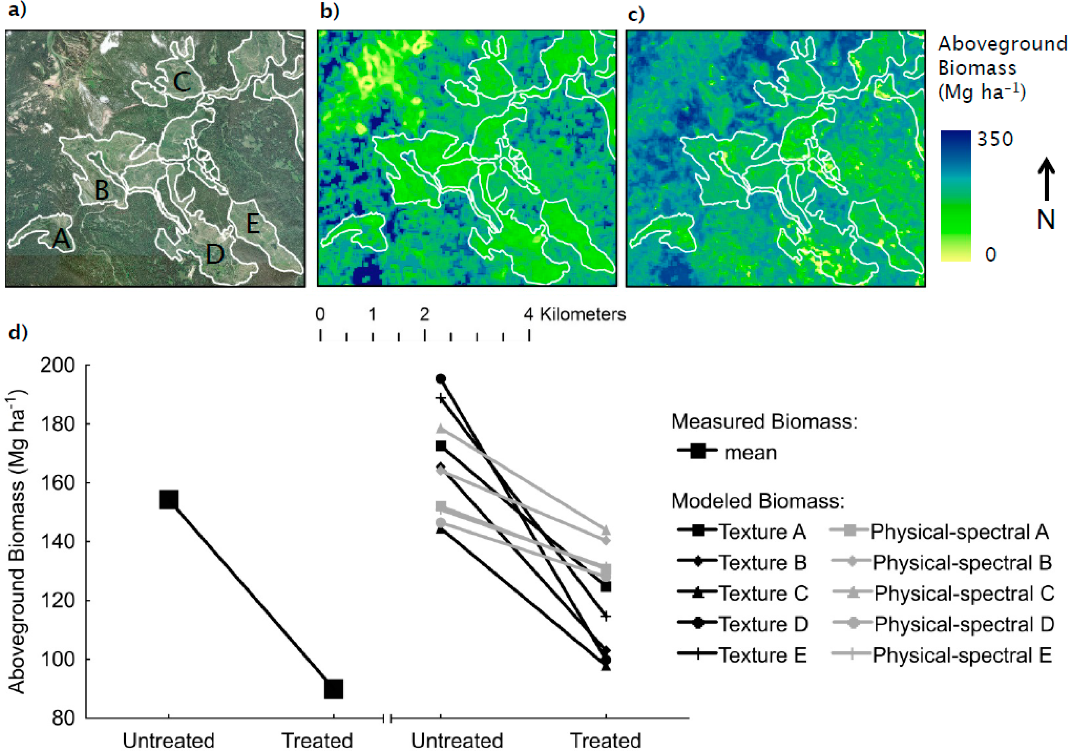
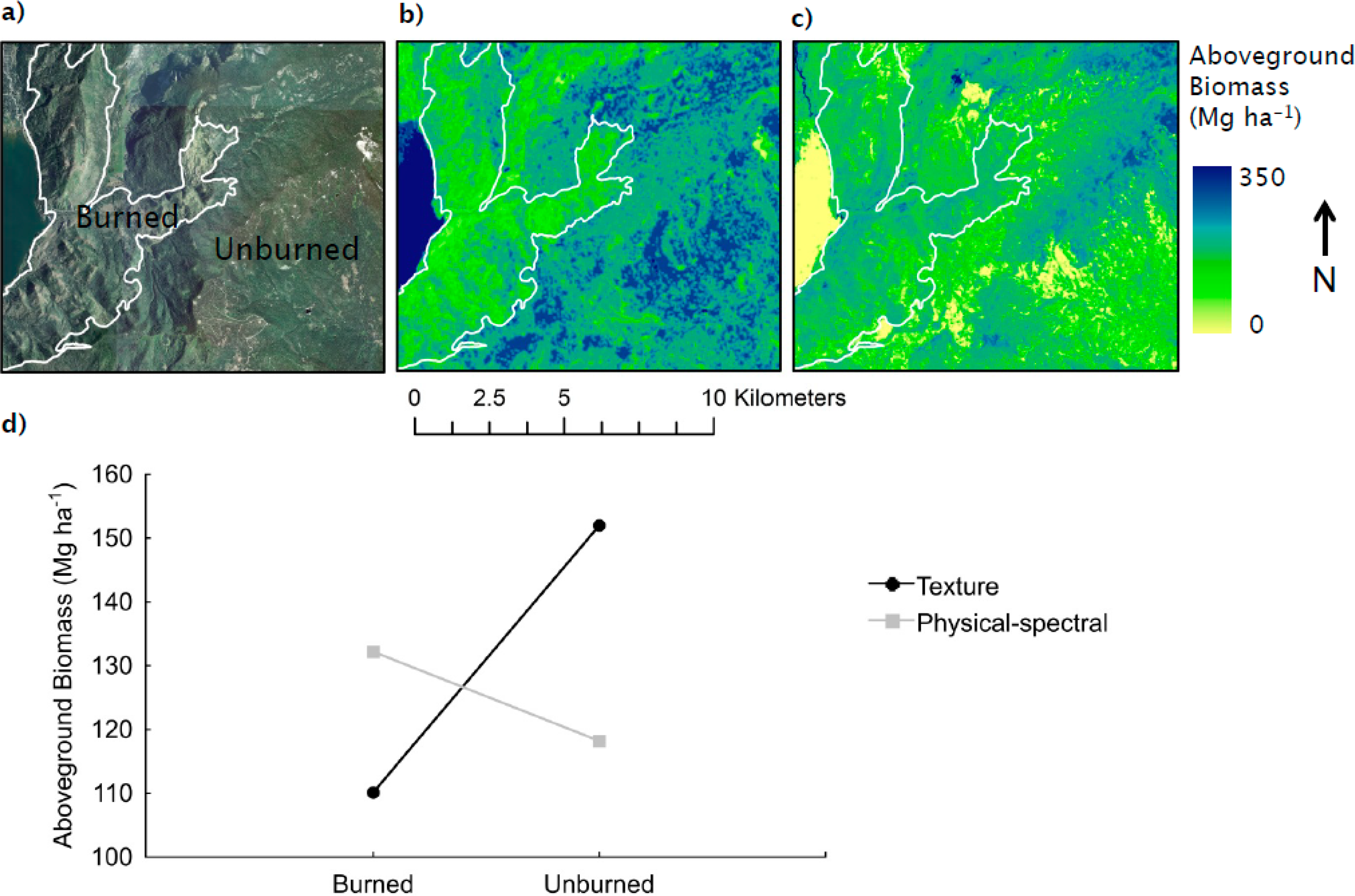
3.2. Biomass Prediction in Areas of Forest Disturbance

The texture-based biomass map also appears better able to capture the magnitude and direction of biomass change due to forest disturbance compared to spectral approaches. Our texture-based map predicted a larger difference in biomass between untreated stands and adjacent clear-cut stands than the physical-spectral map (Figure 4). The observed biomass values suggest an average difference of 64.5 Mg·ha⁻¹ between untreated and clear-cut stands. The texture-based biomass predicted an average difference of 65.3 Mg ha⁻¹ between the clear-cut and untreated stands, whereas the physical-spectral map predicted an average difference of 23.53 Mg ha⁻¹ between the clear-cut and untreated stands (Figure 4).

The texture-based biomass map also improved prediction quality over the physical-spectral map in a region of San Juan National Forest burned in a wildfire in 2002 (Figure 5). In the eastern portion of the Missionary Ridge Fire burn area, the texture-based map predicted a 52.64 Mg·ha⁻¹ decrease in biomass between the burned area and the adjacent unburned forest, where as the physical-spectral based biomass map predicted a 14.0 Mg·ha⁻¹ increase in the amount of biomass present in the burned forest relative to the adjacent unburned forest (Figure 5).

4. Discussion

In this study we demonstrate the utility of image texture analysis on Landsat TM imagery as a method of improving local biomass estimates. Biomass maps including image texture variables perform better than biomass maps created from physical and spectral variables only. Furthermore, our texture-based biomass map is better able to capture biomass change in response to disturbance than maps created excluding image texture. Our analysis provides an alternative avenue for advancing the development of more accurate local biomass maps through a novel application of a widely established remote sensing tool.

4.1. Biomass Prediction from Image Texture

Aboveground biomass predicted by the texture-based model was greatest in high elevation regions, and smallest in the low elevation regions (Figure 3). This pattern is generally spatially consistent with national scale biomass maps for this region [18,31], however, the greatest biomass value predicted by the texture-based map, 394 Mg·ha⁻¹, is lower than the highest observed biomass for this region (490 Mg·ha⁻¹). The correlation between our texture-based model biomass predictions and observed biomass values was r = 0.86 (Table 1; Figure 2).

Our successful use of texture to map biomass in SJNF is encouraging for several reasons. First, our texture-based model was constructed using only publically available data and Landsat TM imagery, whereas most existing biomass maps are constructed from a large suite of geospatial predictors. Although we recognize that many spatial predictors are needed for national scale maps, we suggest that alternate approaches, such as use of texture analysis, may be more appropriate for local maps. Secondly, we believe that texture analysis may be able to improve biomass estimation in regions of forest where spectral indices such as NDVI can saturate. Unlike NDVI, which is calculated on a pixel-by-pixel basis, texture is calculated from a small neighborhood of pixels and the size of this neighborhood can be adjusted to maximize the potential for texture to predict biomass. We find that texture is particularly useful in regions of disturbed forest (Figures 4 and 5), where the texture-based map is more sensitive to changes in forest biomass than a map produced from physical and spectral variables. Furthermore, texture analysis also has the potential to be sensitive to changes in forest biomass even in regions of dense canopy; studies from tropical forests indicate that texture correlates with biomass more strongly than spectral indices [13], and texture is correlated with biomass in some regions where spectral signatures are not [14]. Finally, we also acknowledge the possibility that the success of texture in predicting forest biomass is partially due to the aggregation process of the window used in texture analysis accounting for errors between image geo-rectification and GPS field locations. If the Landsat image is offset by even just one pixel, the plot locations will be 30 m removed from the corresponding pixel in the Landsat image. In this case texture analysis may help account for this geographic error by aggregating pixel values over the window used in texture analysis (i.e., 3 × 3).

There are several opportunities for introduction of error into our texture-based biomass model. First, the ground-based FIA plots used in our model were sampled between 2002 and 2009, whereas the Landsat scenes used for the texture calculation were acquired in 2011. While the Landsat scenes we used in our analysis are temporally consistent with the recently sampled FIA plots, there is almost a 10-year lag between the sampling date of the earliest plots, and the time of Landsat image acquisition. During this time the amount of biomass on the landscape could have changed due to growth or disturbance, thereby introducing error into the resulting map. However, the direction of the map errors (the map under predicts biomass) is not consistent with errors introduced due to forest disturbances that remove biomass, such as forest treatment or wildfire. In the case of disturbances including treatment and wildfire, forest biomass on the landscape would decrease, and therefore the biomass map would over predict forest biomass for disturbed areas. In contrast, our map under predicts forest biomass in some regions.

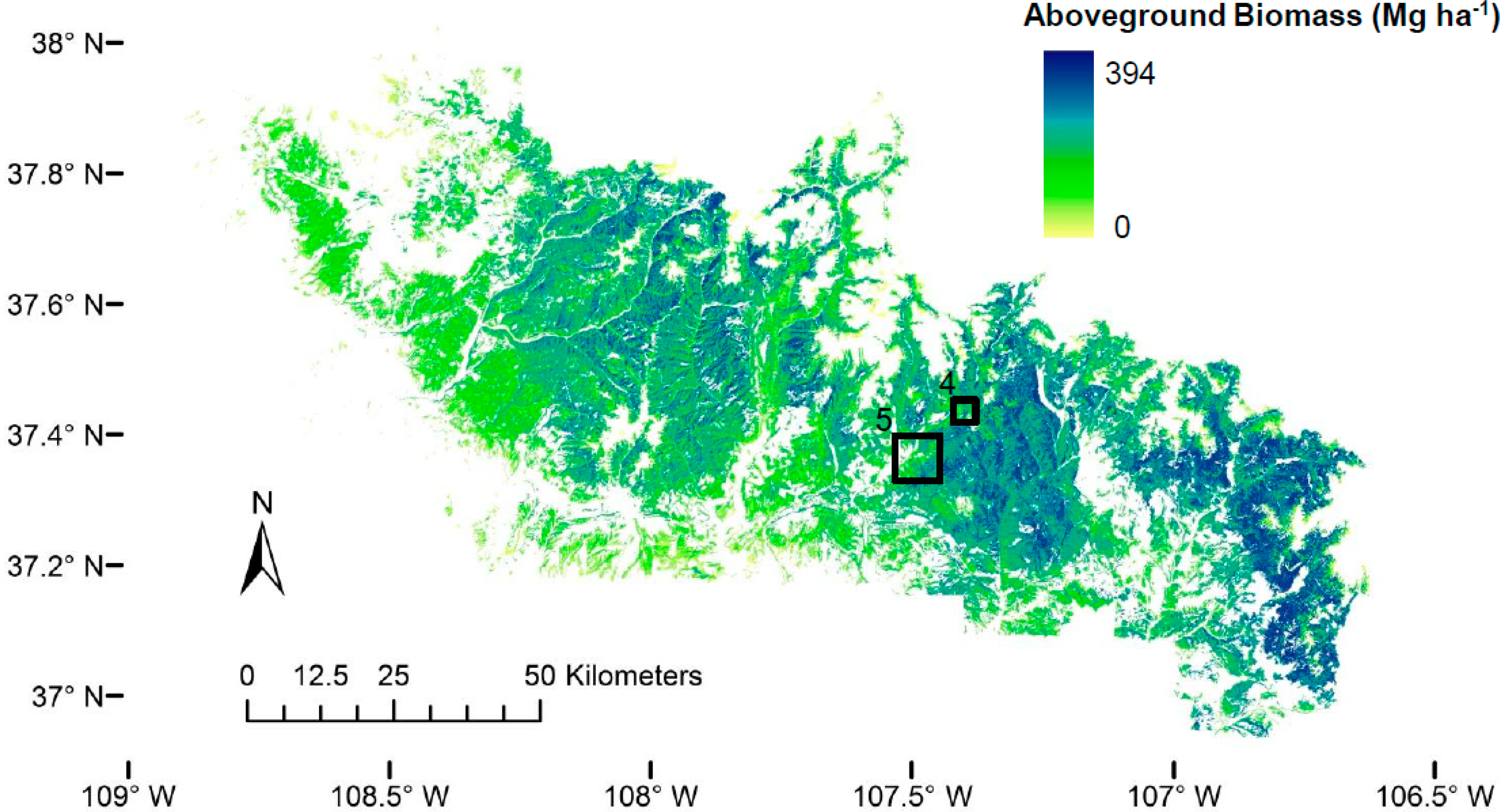
4.2. Texture Analysis for Local Biomass Maps

The texture-based biomass map we present here is an effective method for developing local forest biomass maps, and could have substantial implications for carbon accounting and land management purposes. Local biomass maps are important for tracking biomass stocks and carbon fluxes in regions such as National Forests, which are sites of frequent land management and disturbance. Our texture-based biomass map is particularly sensitive to changes in biomass following disturbance, and actually improves biomass predictions within disturbed regions relative to maps made from exclusively physical and spectral variables. Specifically, the texture-based map produced biomass predictions that closely match observed biomass values from nearby forest stands of the same vegetation type and treatment history (Figure 4). Furthermore, the physical-spectral map predicted an increase in forest biomass in a region of recently burned forest relative to the adjacent unburned forest, whereas the texture-based map predicted a decline in forest biomass in the burned region (Figure 5). We believe this result is due to high prevalence of understory vegetation growing in the burned region, resulting in high NDVI but low biomass. Because texture appears to be sensitive to changes in forest biomass following disturbance in SJNF, we suggest that texture may be an important tool not only for creating biomass maps in regions such as national forests, but also for updating these maps following disturbance or management. The Landsat data used to construct this map are available on sub-annual timescales so map updates are not subject to constraints in data acquisition. Potential future climate change mitigation policies enacted through forest management, or trading schemes introduced under cap-and-trade type policy, will rely on biomass maps to inform decisions, and image texture analysis provides a potential avenue to make necessary improvements to local biomass estimates.

5. Conclusions

Local forest biomass maps are necessary for understanding and anticipating the effects of disturbance and management on forest area, habitat, and local carbon stocks and fluxes. In this study we use a combination of physical variables, spectral information and image texture metrics calculated from Landsat TM imagery to create a local forest biomass map within San Juan National Forest in Southwest Colorado, USA. Aboveground biomass maps were created using neural networks constructed from Forest Inventory and Analysis Program ground-based biomass observations and the corresponding physical, spectral and image texture information for each plot location. We draw the following conclusions:

• Biomass models constructed including image texture variables are more strongly correlated with observed biomass than those constructed using physical and spectral information alone.
• Our texture-based biomass model is sensitive to changes in forest biomass following disturbance such as logging and wildfire; the texture-based model we present in this paper is better able to predict the direction and magnitude of biomass change following disturbance than biomass models constructed without the use of image texture.
• Because the Landsat data used to construct this map are available on sub-annual timescales, texture may be an important tool for creating and updating biomass maps following local forest disturbance or land management actions.
• The methods we present here are widely applicable across the US because we use entirely publically available data processed with relatively simple analytical routines.

The next steps of this research will include evaluating the transferability of this local texture-based biomass model to other geographic regions with varying vegetation and disturbance regimes.

References

1. EPA. Inventory of U.S. Greenhouse Gas Emissions and Sinks: 1990–2009. Available online: http://www.epa.gov/climatechange/Downloads/ghgemissions/US-GHG-Inventory-2011-Complete_Report.pdf (accessed on 7 February 2014).
2. Ryan, M.G.; Harmon, M.E.; Birdsey, R.A.; Giardina, C.P.; Heath, L.S.; Houghton, R.A.; Jackson, R.B.; Mckinley, D.C.; Morrison, J.F.; Murray, B.C.; et al. A synthesis of the science on for U.S. forests. Issues Ecol 2010, 13, 1–16. [Google Scholar]
3. United States Department of Agriculture (USDA), Dimension 4: Mitagation and sustainable consumption. In Navigating the Climate Change Performance Scorecard; USDA: Washington, DC, USA, 2011; pp. 1–103.
4. Goetz, S.J.; Baccini, A.; Laporte, N.T.; Johns, T.; Walker, W.; Kellndorfer, J.; Houghton, R.A.; Sun, M. Mapping and monitoring carbon stocks with satellite observations: A comparison of methods. Carbon Balance Manag 2009, 4. [Google Scholar] [CrossRef]
5. Richards, J.A. Chapter 5: Geometric processing and enhancement: Image domain techniques. In Remote Sensing Digital Image Analysis, 5th ed; Springer: London, UK, 2013; pp. 162–163. [Google Scholar]
6. Le Toan, T.; Beaudoin, A.; Riom, J.; Guyon, D. Relating forest biomass to SAR data. IEEE Trans. Geosci. Remote Sens 1992, 30, 403–411. [Google Scholar]
7. Kasischke, E.S.; Melack, J.M.; Craig Dobson, M. The use of imaging radars for ecological applications—A review. Remote Sens. Environ 1997, 59, 141–156. [Google Scholar]
8. Dubayah, R.O.; Drake, J.B. Lidar remote sensing for forestry. J. For 2000, 98, 44–46. [Google Scholar]
9. Huete, A.R.; van Leeuwen, W.J.D. The use of vegetation indices in forested regions: Issues of linearity and saturation. Proceedings of the 1997 IEEE International Geoscience and Remote Sensing Symposium. Remote Sensing—A Scientific Vision for Sustainable Development (IGARSS’97), Singapore International Convention & Exhibition Centre, Singapore, 3–8 August 1997; 4, pp. 1966–1968.
10. Ouchi, K. Recent trend and advance of synthetic aperture radar with selected topics. Remote Sens 2013, 5, 716–807. [Google Scholar]
11. Lim, K.; Treitz, P.; Wulder, M.; St-Onge, B.; Flood, M. LiDAR remote sensing of forest structure. Prog. Phys. Geogr 2003, 27, 88–106. [Google Scholar]
12. Cutler, M.E.J.; Boyd, D.S.; Foody, G.M.; Vetrivel, A. Estimating tropical forest biomass with a combination of SAR image texture and Landsat TM data: An assessment of predictions between regions. ISPRS J. Photogramm. Remote Sens 2012, 70, 66–77. [Google Scholar] [Green Version]
13. Eckert, S. Improved forest biomass and carbon estimations using texture measures from WorldView-2 satellite data. Remote Sens 2012, 4, 810–829. [Google Scholar]
14. Lu, D. Aboveground biomass estimation using Landsat TM data in the Brazilian Amazon. Int. J. Remote Sens 2005, 26, 2509–2525. [Google Scholar]
15. PRISM Climate Data, 2013. Available online: http://www.prism.oregonstate.edu (accessed on 1 November 2013).
16. San Juan National Forest, Geospatial Data 2013. Available online: http://www.fs.usda.gov/main/sanjuan/landmanagement/gis (accessed on 15 February 2013).
17. ArcGIS Services Directory, 2013. Available online: http://server.arcgisonline.com (accessed on 15 December 2013).
18. Blackard, J.; Finco, M.; Helmer, E.; Holden, G.; Hoppus, M.; Jacobs, D.; Lister, A.; Moisen, G.; Nelson, M.; Reimann, R. Mapping U.S. forest biomass using nationwide forest inventory data and moderate resolution information. Remote Sens. Environ 2008, 112, 1658–1677. [Google Scholar]
19. Forest Inventory and Analysis National Program, Data-Mart 2013. Available online: http://www.fia.fs.fed.us/tools-data/ (accessed on 1 October 2012).
20. Hoppus, M.; Lister, A. The status of accurately locating forest inventory and analysis plots using the Global Positioning System. Proceedings of the Seventh Annual Forest Inventory and Analysis Symposium, Portland, OR, USA, 3–6 October 2005; pp. 179–184.
21. Jenkins, J.C.; Chojnacky, D.C.; Heath, L.S.; Birdsey, R.A. Comprehensive database of diameter-based biomass regressions for North American tree species. In General Technical Report NE-319; United States Department of Agriculture, Forest Service, Northeastern Research Station: St. Paul, MN, USA, 2004. [Google Scholar]
22. Kaye, J.P.; Hart, S.C.; Fulé, P.Z.; Covington, W.W.; Moore, M.M.; Kaye, M.W. Initial carbon, nitrogen, and phosphorus fluxes following ponderosa pine restoration treatments. Ecol. Appl 2005, 15, 1581–1593. [Google Scholar]
23. Chander, G.; Markham, B.L.; Helder, D.L. Summary of current radiometric calibration coefficients for Landsat MSS, TM, ETM+, and EO-1 ALI sensors. Remote Sens. Environ 2009, 113, 893–903. [Google Scholar]
24. Chavez, P.S. An improved dark-object subtraction technique for atmospheric scattering correction of multispectral data. Remote Sens. Environ 1988, 24, 459–479. [Google Scholar]
25. Teillet, P.M.; Guindon, B.; Goodenough, D.G. On the slope-aspect correction of multispectral scanner data. Can. J. Remote Sens 1982, 8, 84–106. [Google Scholar]
26. USGS National Elevation Dataset 2014. Available online: http://ned.usgs.gov (accessed on 10 March 2014).
27. Haralick, R.M.; Shanmugam, K.; Dinstein, I. Textural features for image classification. IEEE Trans. Syst. Man. Cybern 1973, 3, 610–621. [Google Scholar]
28. Lu, D.; Batistella, M. Exploring TM image texture and its relationships with biomass estimation in Rondônia, Brazilian Amazon. Acta Amaz 2005, 35, 249–257. [Google Scholar]
29. Clausi, D.A. An analysis of co-occurrence texture statistics as a function of grey level quantization. Can. J. For. Res 2002, 28, 45–62. [Google Scholar]
30. Spendelow, J.A.; Nichols, J.D.; Nisbet, I.C.T.; Hays, H.; Cormons, G.D. Estimating annual survival and movement rates of adults within a metapopulation of roseate terns. Ecology 1995, 76, 2415–2428. [Google Scholar]
31. Kellndorfer, J.; Walker, W.; LaPoint, E.; Bishop, J.; Cormier, T.; Fiske, G.; Hoppus, M.; Kirsh, K.; Westfall, J. NACP Aboveground Biomass and Carbon Baseline Data. 2000. Data Set. Available online: http://daac.ornl.gov/NACP/guides/NBCD_2000.html (accessed on 11 June 2013).
Figure 1. Location of San Juan National Forest within southwest Colorado, and distribution of Forest Inventory and Analysis plots within San Juan National Forest. Scale bar applies to regional San Juan National Forest map. Base map for San Juan National Forest extent: ESRI shaded relief imagery [17]. Projection: Albers NAD83.
Remotesensing 06 06407f1
Figure 2. Observed versus predicted biomass values for Landsat TM image texture based biomass map.
Remotesensing 06 06407f2
Figure 3. Landsat TM image texture-based map of aboveground biomass within forested regions of San Juan National Forest. The boxes labeled 4 and 5 indicate the location of Figures 4 and 5, respectively.
Remotesensing 06 06407f3
Figure 4. (a) True color image from National Agricultural Imagery Program acquired by a Leica ADS80 Airborne Digital Sensor; (b) image texture-based biomass map; and (c) physical-spectral (slope, aspect, elevation, Normalized Difference Vegetation Index) based biomass map for a region of San Juan National Forest containing forested stands clear-cut in the 1970s. Color bar and scale bar apply to (a), (b), and (c); (d) Observed and modeled stand-average aboveground biomass from adjacent untreated and treated (clear-cut) forest stands. Observed values are calculated from nearby stands of the same vegetation type. Modeled stand-average biomass of treated stands was compared to the stand-average biomass of the untreated stand located directly to the west. Letters indicate locations of biomass comparisons, shown on (a).
Remotesensing 06 06407f4
Figure 5. (a) True color image from National Agricultural Imagery Program, acquired by a Leica ADS80 Airborne Digital Sensor; (b) image texture-based biomass map; and (c) physical-spectral (slope, aspect, elevation, Normalized Difference Vegetation Index) based biomass map for a region of San Juan National Forest burned by a wildfire in 2002. Color bar and scale bar apply to (a), (b), and (c); (d) Modeled stand-average biomass of the burned region was compared to the unburned region to the East of the fire.
Remotesensing 06 06407f5