Urban Built-Up Area Extraction from Landsat TM/ETM+ Images Using Spectral Information and Multivariate Texture


Abstract
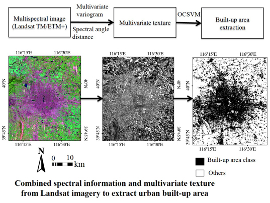
: Urban built-up area information is required by various applications. However, urban built-up area extraction using moderate resolution satellite data, such as Landsat series data, is still a challenging task due to significant intra-urban heterogeneity and spectral confusion with other land cover types. In this paper, a new method that combines spectral information and multivariate texture is proposed. The multivariate textures are separately extracted from multispectral data using a multivariate variogram with different distance measures, i.e., Euclidean, Mahalanobis and spectral angle distances. The multivariate textures and the spectral bands are then combined for urban built-up area extraction. Because the urban built-up area is the only target class, a one-class classifier, one-class support vector machine, is used. For comparison, the classical gray-level co-occurrence matrix (GLCM) is also used to extract image texture. The proposed method was evaluated using bi-temporal Landsat TM/ETM+ data of two megacity areas in China. Results demonstrated that the proposed method outperformed the use of spectral information alone and the joint use of the spectral information and the GLCM texture. In particular, the inclusion of multivariate variogram textures with spectral angle distance achieved the best results. The proposed method provides an effective way of extracting urban built-up areas from Landsat series images and could be applicable to other applications.1. Introduction
Over the past three decades, urban areas in China have been expanding at an unprecedented pace, due to significant economic development. As urban development initiatives encroach on previously un-developed land, the cumulative impact has resulted in the loss of valuable agricultural land, wetland and forest and also an increase in energy consumption and greenhouse gas emission [1]. In order to assess the spatial and temporal nature of urbanization and land-cover change occurring across urban landscapes, city planners, decision-makers and researchers require timely and accurate information.
Remote sensing technologies provide a reliable source for urban land cover/land use data acquisition. In particular, the United States’ NASA Landsat satellite data series (e.g., MSS, TM and ETM+) have been widely used for mapping urban extent and monitoring urban growth [2–7], due to the sensors’ capacity for synoptic view, repeat coverage over large areas and the availability of historical archive imagery [8]. Landsat sensors provide some advantages for the purposes of urban land mapping and change detection in terms of efficiency, as a single image can provide a synoptic view of an area of interest. In comparison to expensive higher-resolution sensors, the comparatively low-resolution nature of the Landsat TM/ETM+ sensor (30 m × 30 m) avoids complications from sparse coverage, limited scene availability and lack of data prior to 2000 when monitoring change for multiple periods. However, mapping urban areas using Landsat TM/ETM+ data remains a complex challenge [9], as there are few thematically pure urban pixels due to the mixture of manmade and vegetative land cover components that comprise urban areas. Complicating matters further, urban areas often display heterogeneous spectral characteristics and significant spectral confusion with other land cover classes: for example, barren land and asphalt concrete share similar spectral characteristics and, as a result, can be readily confused.
Over the past few decades, various methods for urban built-up area extraction have been developed using Landsat TM/ETM+ data. Generally, there are three main categories of urban built-up area extraction methods. First, spectral indexes (i.e., calculated from the spectral information of remotely sensed images) or spatial indexes (e.g., texture), such as the built-up area index or the impervious surface related index, have been proposed and used to extract urban areas [10–16]. However, most existing spectral/spatial indexes mainly focus on the urban class itself, without full consideration of other land cover types; as such, these methods do not successfully address the confusion between urban area and other land cover types. In the second category, combined spectral data and spatial information, such as the combination of road density and spectral information or the combination of spectral data and texture information, are used in the extraction of urban built-up area [2,12,17–19]. However, these existing studies employing single-band texture information did not consider spatial variations between bands [20,21]. In the third category, multi-sensor data, such as Landsat TM/ETM+ and SAR (synthetic aperture radar) data are combined in urban built-up area extraction [4,7,22–27]. Due to the difficulties encountered in synthesizing different data sources, as well as the time-consuming co-registration requirements for multi-sensor images, the methods of multi-sensor data combination have not been used widely.
Image texture is an important source of spatial information that can be derived from images [20]. Texture data, such as classical one-band texture (e.g., gray-level co-occurrence matrix (GLCM) texture), provide additional information for land cover mapping and have been widely used in diverse applications, including urban built-up area extraction [2,12,14,28–30]. However, since each band of a multispectral image generates band-specific texture data, the resultant texture bands have varying capabilities to discriminate between land cover types. The inclusion of one-band texture may not take full advantage of the available texture information contained in the multispectral image. In contrast, multivariate texture (or multi-band texture), e.g., measured by multivariate variogram, extracted simultaneously from all available spectral bands of a multispectral image [31], identifies the spatial variation of multiple bands, thus avoiding the need to select a single band as required in the traditional one-band texture method [21]. The multivariate texture data provide useful spatial information for discriminating between land cover types [31] and have been used in land cover classification, lithological mapping and urban damage assessment [31–34]. In previous studies, Euclidean distance and Mahalanobis distance were used in multivariate variogram texture computation and showed similar performances in land cover classification [31]. However, these two distance measures are sensitive to illumination variations [35], which could be produced by shadow and other factors in rugged terrain [36] and urban area. In contrast, the spectral angle distance [37–39] is insensitive to illumination and albedo effect. As such, the use of spectral angle distance in a multivariate variogram may provide an alternative method for multivariate texture extraction. Thus, the main objective of this study is to combine multivariate variogram texture and spectral data for urban built-up area extraction. The second objective is to investigate if the use of different distance measures in a multivariate variogram for multivariate texture extraction affects the performance of multivariate texture in combined classification for urban area mapping. The third objective is to evaluate the ability of this method in using historical archive Landsat imagery to the application of built-up area extraction
The term “urban area” is widely used in the literature and refers to the spatial extent of urbanized areas on a regional scale, but this is a fuzzy and inconsistent definition [7]. Since urban areas are mainly dominated by built-up lands with impervious surfaces, in this study, urban built-up area is used to represent the area directly occupied by a particular physical structure, including buildings, streets and impervious surfaces, all man-made structures, i.e., a “settlement mask” [7,24].
2. Methods
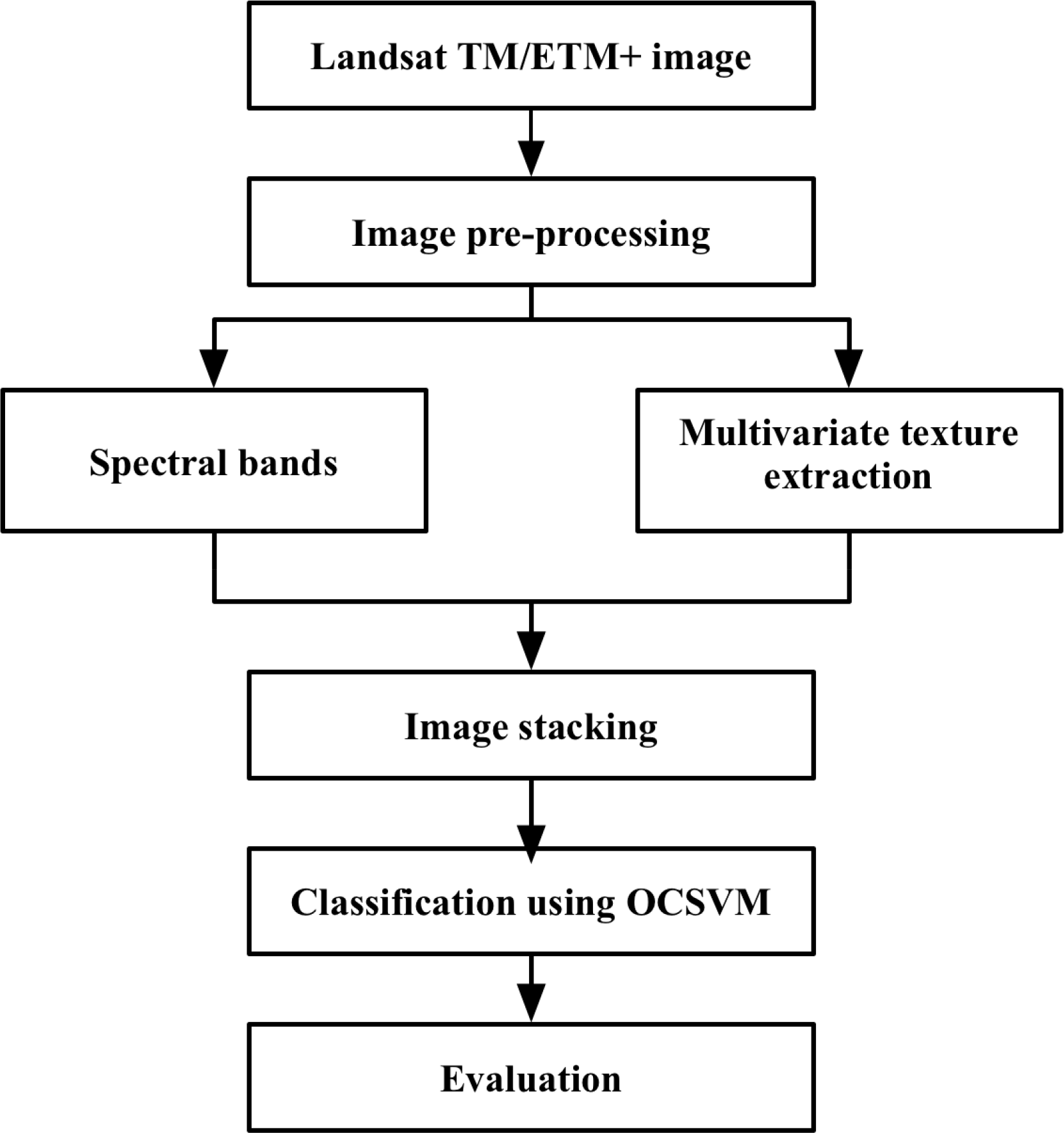
As mentioned previously, the main purpose of this study is to combine multi-band spectral data and multivariate texture information for the extraction of urban built-up areas using the Landsat series data. The main idea can be summarized as follows (Figure 1). First, multivariate variogram texture [31] is extracted from a Landsat TM/ETM+ multispectral image (Section 2.1), and then, the obtained multivariate texture is combined with the original multispectral image as an additional band. The combined spectral and texture images are classified to extract urban built-up area (Section 2.2). A one-class classifier, one-class support vector machine (OCSVM), is used in the classification (Section 2.2). To demonstrate the effectiveness of the proposed method, the image texture measured by the classical GLCM is also used in the extraction of the built-up area for comparison.
2.1. Multivariate Texture Calculation
In this study, multivariate texture was measured using the multivariate variogram [31,40]. The multivariate variogram summarizes the spatial variations of multiple variables (e.g., spectral bands of a multispectral image) [40].
From a perspective of geostatistics, the digital number (DN) of a remote sensing image is considered as a regionalized variable, characterized by both random and spatial correlation aspects [41]. For a multispectral image that can be modeled as multivariate data, each pixel can be viewed as a vector of p spectral bands (variables):
The multivariate variogram with Euclidean distance is expressed as:
The multivariate variogram with Mahalanobis distance is defined as:
In addition to the Euclidean distance and the Mahalanobis distance, the spectral angle distance [37,42], which has not been used for the extraction of multivariate texture in existing studies, is also used in this paper. The multivariate variogram with the spectral angle distance is expressed as:
The multivariate texture was calculated in a local neighborhood (i.e., moving window) from all multispectral bands using Equations (3)–(5), respectively. There are two parameters to be considered when calculating multivariate texture: the window size and the lag distance (including distance and direction) [31]. The obtained multivariate variogram value (for a specified moving window and a lag distance) is assigned to the central pixel of the window. The selection of an appropriate window size is usually done by a trial and error procedure. Generally, multiple lag distances can be used in the calculation of a multivariate variogram. However, it was found from the existing studies that the lag distance of one pixel is widely used for geostatistical texture computation, because it best describes the radiometric differences in the immediate neighborhood of the central pixel [21]. However, other lag distances can also provide useful information [43]. Usually, the lag distance can be measured in individual directions or in multiple directions within a moving window. In most previous studies, the omnidirectional texture that is produced by averaging the texture values from several directions (e.g., NS, EW, NE-SW, NW-SE) was used [21,31]. However, omnidirectional texture usually shows severe edge effect, which is a well-known problem associated with the use of texture measures [12,34,44]. Thus, in this study, the minimum texture, i.e., the minimum of the texture values for different directions, is used, since it is less sensitive to the edge effect [12]. It should be mentioned that since only one lag distance value was used in the multivariate variogram in this study, the multivariate texture obtained is actually the multivariate semivariance texture.
2.2. Urban Built-Up Area Extraction Using Combined Spectral and Texture Information
The obtained multivariate variogram texture and original multispectral image are combined for urban built-up area extraction. The combination is done by a vector stack method, i.e., the derived multivariate variogram texture image is combined with spectral data as an additional band. For example, if there are six spectral bands of the original image and an extracted multivariate variogram texture band, the combined data will have seven bands. In this paper, multivariate textures measured using the multivariate variogram with three different distances (i.e., Euclidean distance, Mahalanobis distance and spectral angle distance) are separately combined with spectral information. Thus, three data combinations are produced. In addition, to fully validate the performance of the proposed method, two other data combinations are used for comparison: (1) spectral information alone; and (2) spectral information and the one-band GLCM texture feature. There are five kinds of data combinations in total.
Since the spectral and texture features generally have different data ranges, the classification process may be dominated by data sources that display a larger scale of variation [45]. With such different data ranges, the classification directly using the original spectral features and the textural features may not achieve a satisfactory classification result. Therefore, prior to classification, both spectral and texture features are first normalized into the same range [0, 1]. The normalization can be formulated as:
The combined spectral and texture images are classified using a supervised classifier to extract urban built-up area. Since the urban built-up area is the only class of interest (or target class), instead of using traditional multi-class classification methods, a one-class classifier, OCSVM, is adopted in this study.
The OCSVM is a recently developed one-class classifier, which is a special type of classical binary support vector machine (SVM). The OCSVM classifier only requires training data from one class (the target class) and can especially focus on the class. In the training process, only samples from the target class are used, and there is no information about outlier objects. The boundary between the target class and others has to be estimated from data in the only available target class. Thus, the task is to define a boundary around the target class; the boundary encircles as many target examples as possible and minimizes the chance of accepting outlier objects [33,46]. Furthermore, the OCSVM classifier is adopted in this study since it has also been successfully applied in specific land cover type mapping [47], change detection of one specific land cover class (e.g., urban expansion and urban building damage detection) [33] and ecological modeling [48].
2.3. Accuracy Assessment
A common method for accuracy assessment is the use of a confusion matrix. For each classification result of different data combinations, the accuracy assessment includes the producer’s accuracy (PA), user’s accuracy (UA), overall accuracy (OA) and kappa coefficient. The kappa coefficient is a measure of the overall statistical agreement of a matrix and takes non-diagonal elements into account. Kappa analysis has been recognized as a powerful technique for analyzing a single error matrix and comparing different confusion matrices [49,50]. In this study, McNemar’s test was used to evaluate the statistical significance of the difference between two classification results using the same set of reference data [51]. If the test value, |Z|, is greater than 1.96, the two classification results produce significantly different accuracies at a 95 percent confidence interval.
3. Study Areas and Data
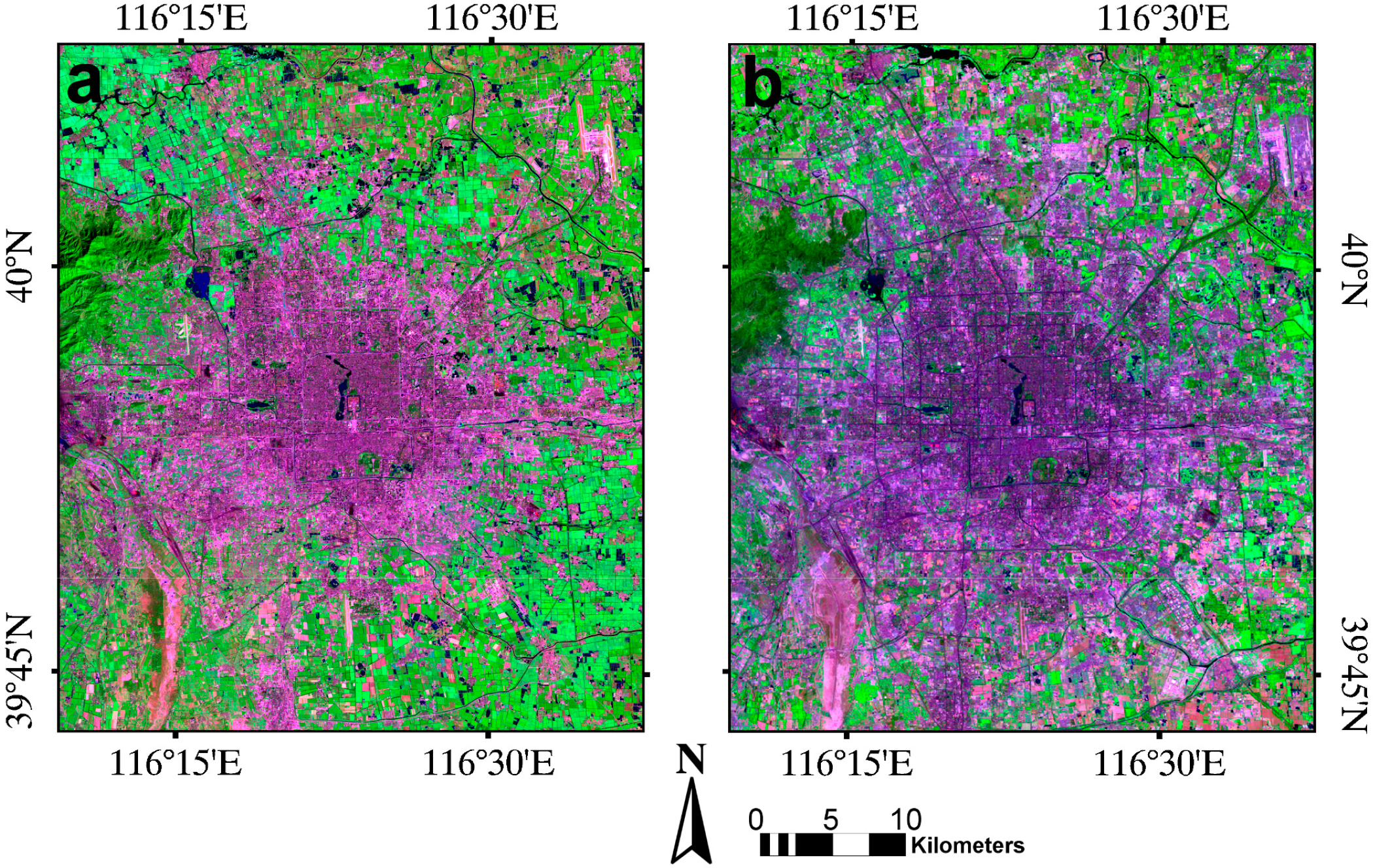
Two megacity areas in China, Beijing and Tianjin, were selected as study areas for the evaluation of the proposed method. Beijing, the capital city of China, is located in northern China. Beijing has experienced a rapid urbanization in the past three decades, resulting in increased infrastructural and housing construction and urban expansion. The land cover types in the area include water, farmland, grassland, woodland, built-up area and bare land.
Bi-temporal Landsat TM/ETM+ data that were acquired in September 1995, and in July 2005, were used. Only six reflective multispectral bands (Bands 1–5, 7) with 30-m spatial resolution were used for each image. The image is free of clouds and of a high quality. No radiometric correction was conducted, since land cover classification does not gain from radiometric correction [52]. Bi-temporal images were co-registered. The image size finally used in the study is 1600 × 1860 pixels, covering an area of approximately 48 km × 55.8 km (Figure 2). The training samples for the target class (built-up area) were visually selected from bi-temporal images. For accuracy assessment, 500 randomly distributed pixels were first generated for both built-up area and non-built-up area classes. After removing the pixels that were located near class boundaries and difficult in the determination of their class attributes and that were near the training pixels, a small polygonal area (cluster) (approximately 80–110 pixels each) around each remaining pixel was then selected as a test area. The training and test samples for the bi-temporal images of Beijing are shown in Table 1.
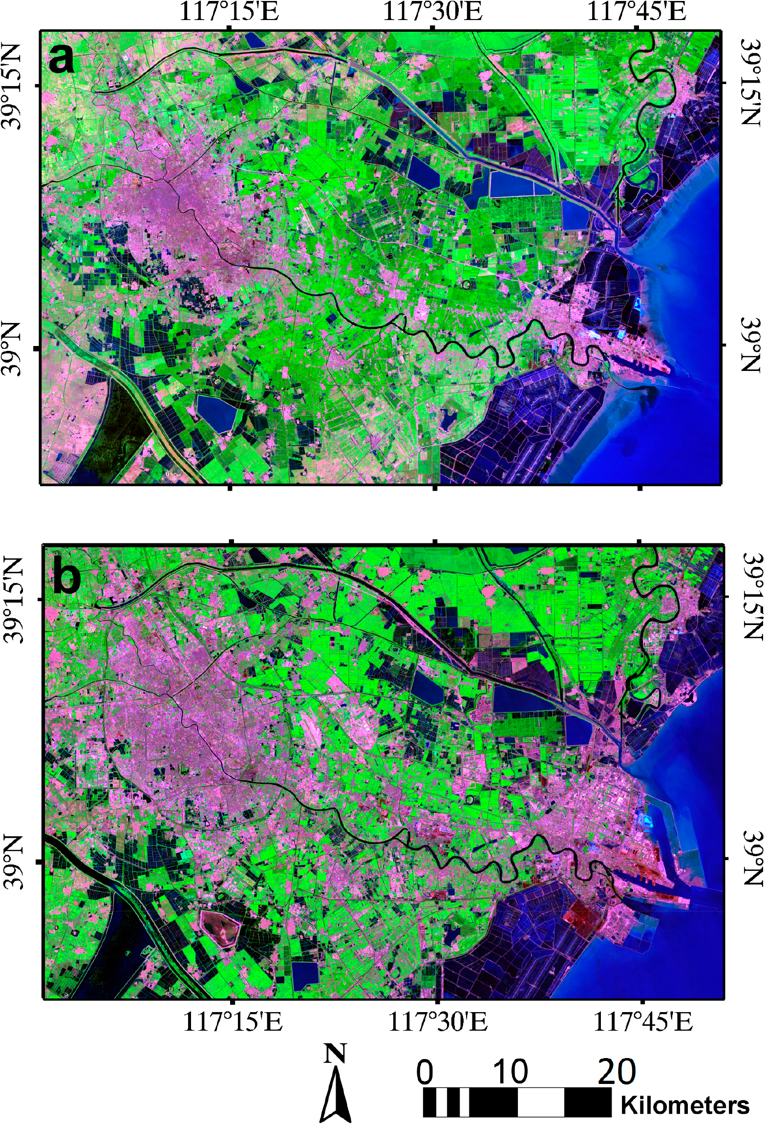
The other study area, Tianjin, is also located in northern China. Tianjin is the third largest city and the second port city of China, which has experienced rapid urban and industrial development over twenty years. The land cover types in the area are the same as those in Beijing area. Two-temporal Landsat TM/ETM+ data acquired in July 1992, and in July 2006, were selected. Only six reflective multispectral bands (Bands 1–5, 7) with 30-m spatial resolution were used. The image is free of clouds and of a good quality. After image registration, the image size used in the study is 2400 × 1600 pixels, covering an area of approximately 72 km × 48 km (Figure 3). The training and test samples were selected following the same procedure used for Beijing images. The training and test samples for bi-temporal images of Tianjin are shown in Table 1.
4. Results and Discussion
4.1. Built-Up Area Extraction Results in Beijing
The multivariate variogram texture was first extracted. In order to choose an appropriate window size for the final texture computation and subsequent combined classification, several window sizes, i.e., 3 × 3, 5 × 5, 7 × 7, 9 × 9 pixels, with a lag distance of one pixel, were respectively used to calculate image textures, which were compared in terms of the accuracy of the combined classification. Considering that spatial variations for these two areas are similar, the Landsat TM image of 2005 was used to estimate the optimal window size. The classification accuracies produced using spectral data and multivariate variogram texture data with different window sizes are shown in Table 2.
From Table 2, it was found that the window size of 7 × 7 pixels used for texture calculation generally achieved the highest kappa coefficient among all window sizes. Hence, the window size of 7 × 7 pixels with a lag distance of one pixel was finally used in the multivariate variogram texture calculation.
In addition, eight GLCM textures were also calculated, namely mean, variance, homogeneity, contrast, dissimilarity, entropy, second moment and correlation. As in many existing studies, the red band and near-infrared (NIR) band were used to compute eight GLCM textures [38,53]. In the process of GLCM texture calculation, a window size of 7 × 7 pixels and a one pixel offset for all directions were computed; the minimum of the texture values for different directions was finally used. After visual inspection and quantitative comparison, the dissimilarity texture computed from the NIR band was used in subsequent analysis, since it achieved the highest accuracy among all combined spectral and GLCM texture classifications (Table 3).
Table 4 shows classification accuracies using different data combinations from the Beijing images. From the table, the classification using spectral information alone produced the lowest accuracies, with kappa coefficients of 75.82% and 77.96% for the 1995 and 2005 images, respectively. By adding textures, either one-band texture (GLCM dissimilarity) or multivariate textures, the classification accuracies were highly improved compared to the use of spectral information alone. For example, by adding one-band texture (GLCM dissimilarity), the increases in the kappa coefficient were 5.14% and 1.02% for the 1995 and 2005 images, respectively. Furthermore, by adding multivariate textures, the accuracies of combined classification were higher than that of classification including one-band texture. In particular, the inclusion of multivariate texture with spectral angle distance in combined classification achieved the highest accuracy among the results of adding one of three multivariate textures. For example, compared to the results using spectral information alone, the increases in the kappa coefficient were 5.07% and 8.67% for the 1995 and 2005 images, respectively; while compared to the results using spectral information and one-band texture, the increases in the kappa coefficient were 2.07% and 5.51% for the 1995 and 2005 images, respectively (Table 4).
Table 5 shows |Z| values from McNemar’s test for Beijing images, which were used to quantify the statistical significance of the difference between the two classification results. From Table 5, it is clear for two images that, compared with the classification results using spectral information alone, all classification results using combined spectral information and texture (GLCM or multivariate variogram) achieved significantly higher accuracies (at the 95% confidence level). Furthermore, the classification result using spectral information and multivariate variogram texture with spectral angle distance generated significantly higher accuracy than all other combinations of spectral data and texture (both GLCM and multivariate variograms with Euclidean and Mahalanobis distances).
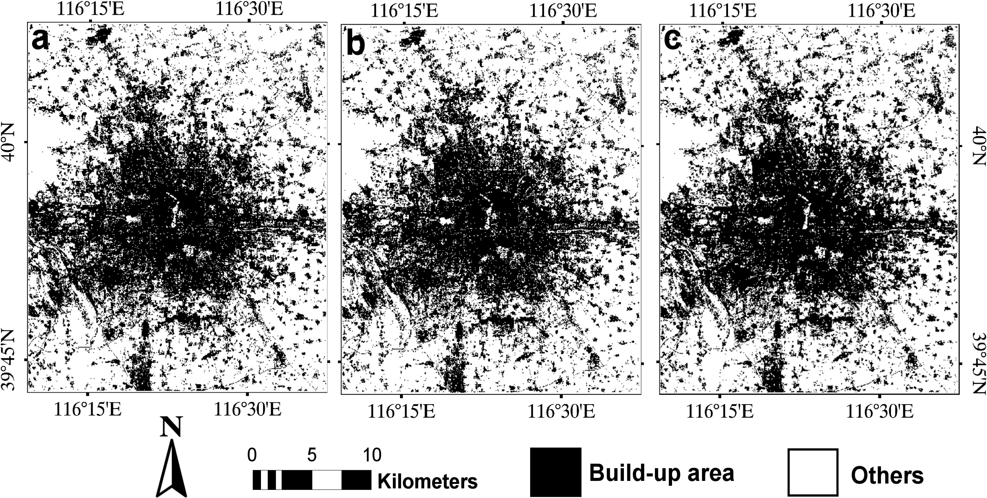
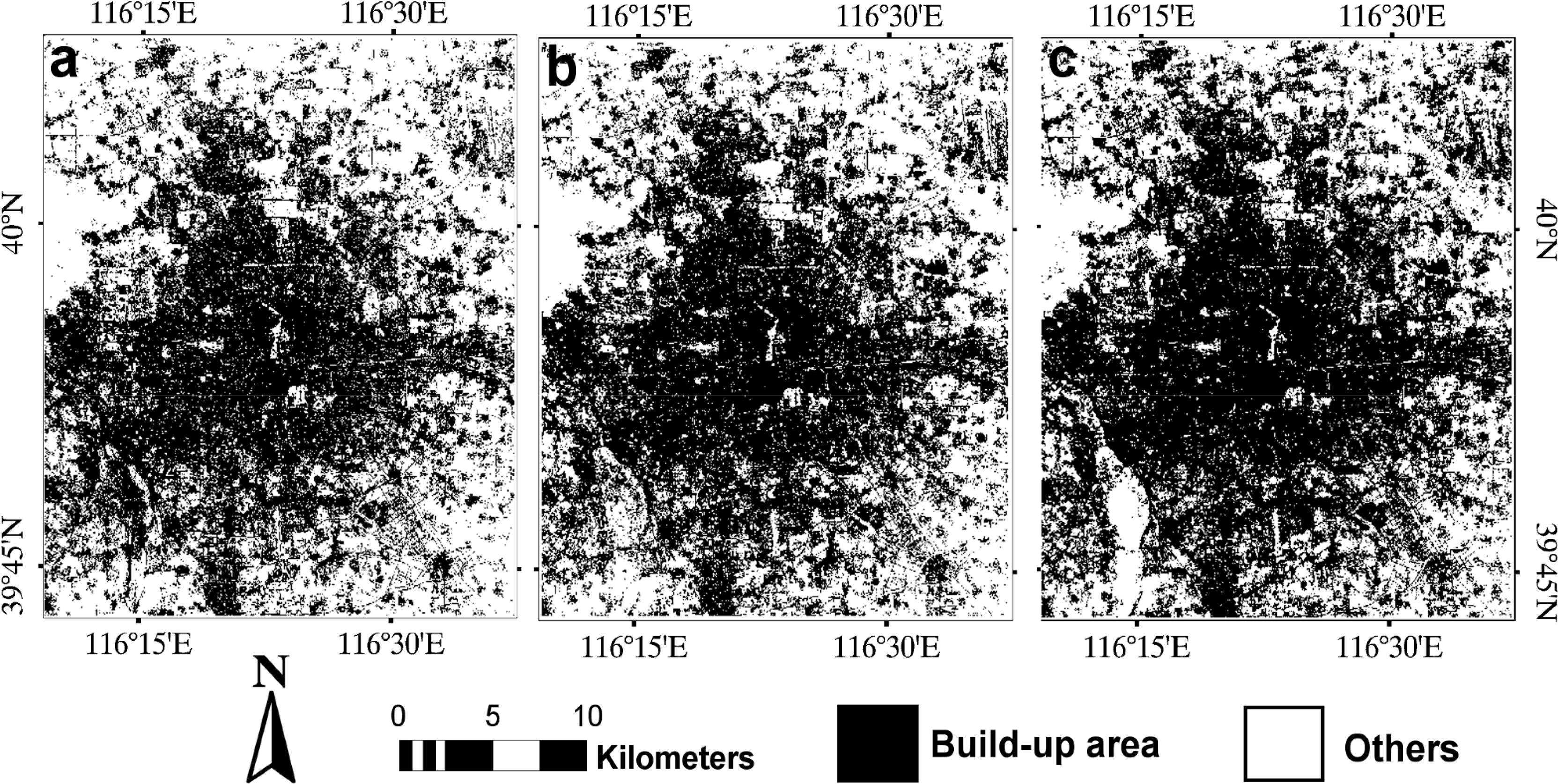
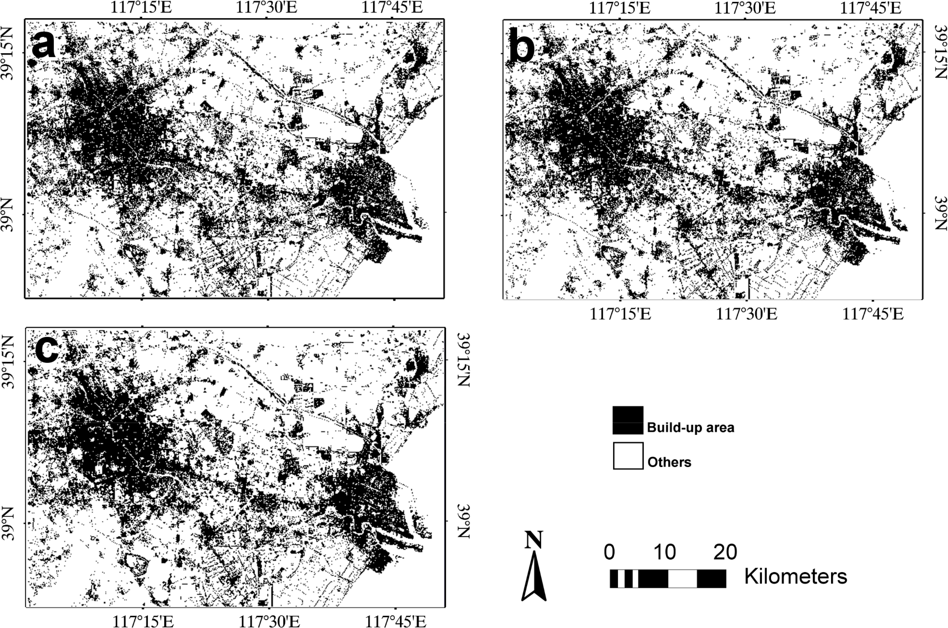
Figures 4 and 5 show the three selected classification results for the 1995 and 2005 images of the Beijing area, respectively. For the 1995 image, it is seen that the results using different data combinations have a similar distribution of the built-up area over the whole scene (Figure 4). For the 2005 image, one obvious difference among these results is shown in the lower left region of three images: there is an area that was labeled as different classes by different methods (Figure 5). For two sets of results, differences among each set of results usually happened in detailed local regions, such as in rural settlement areas, harvested farmland area and built-up area that has unusual spectral information corresponding to surrounding built-up areas. Thus, some local places in each image have been selected for comparison (Figure 6).
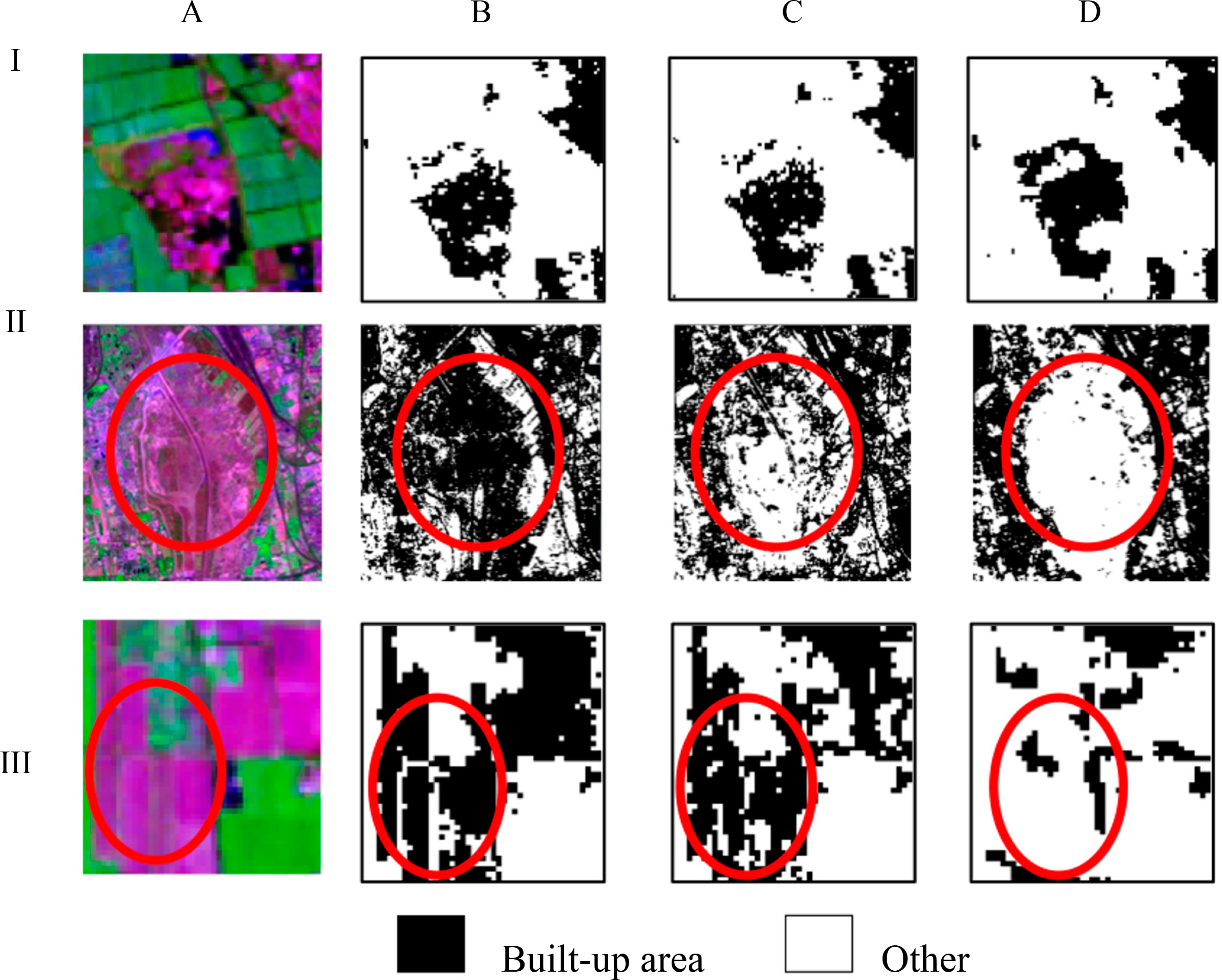
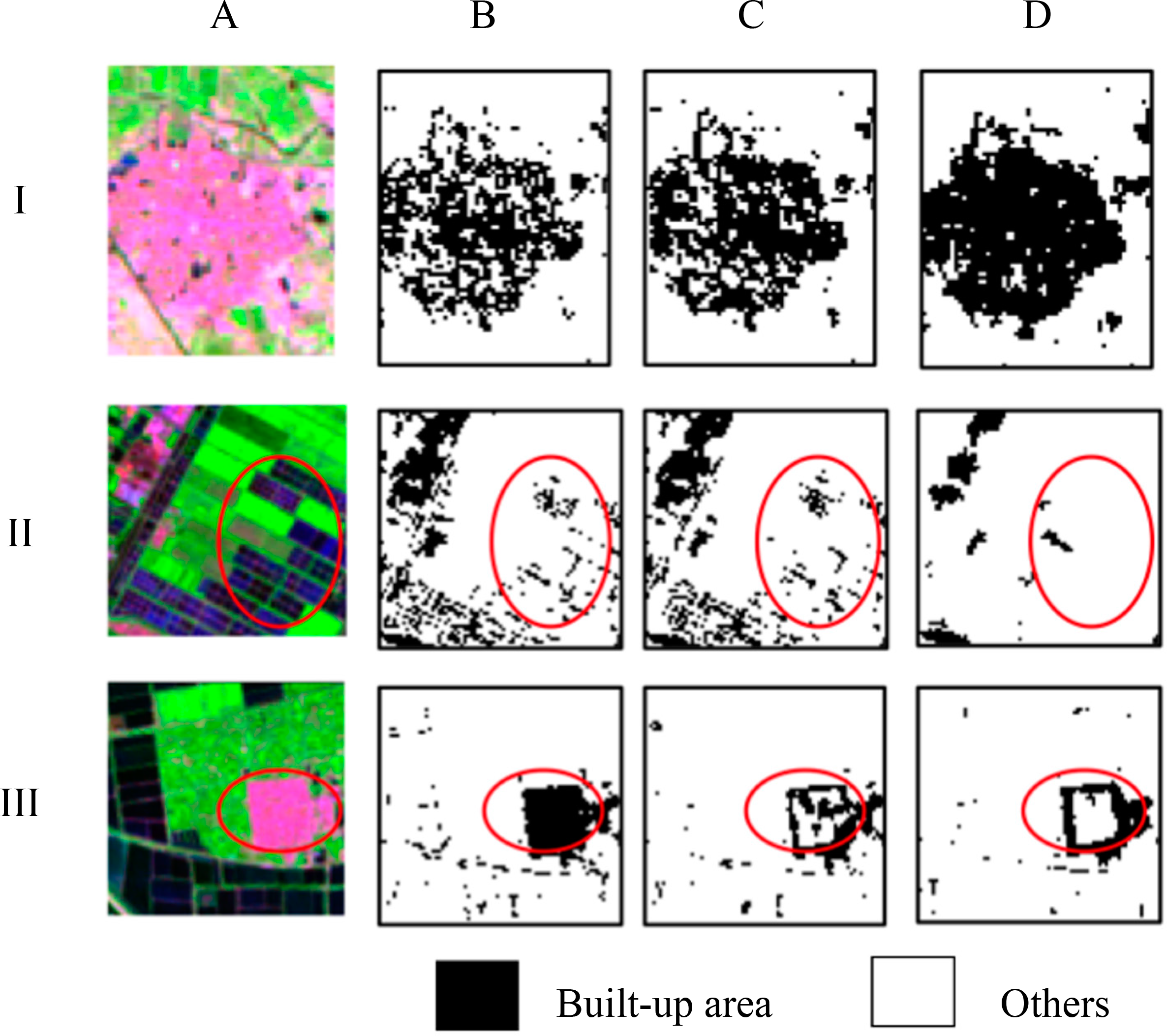
From Figure 6, by using spectral data alone and using combined spectral data and GLCM texture, the urban built-up areas were partially recognized (e.g., I-B, I-C of Figure 6). However, when spectral data and multivariate variogram texture were jointly used, the built-up area was more accurately extracted. When spectral data were used alone, some areas of bare land and harvested land were misclassified as urban built-up area (e.g., II-B, III-B of Figure 6). When GLCM texture was included in classification, the misclassification error was slightly reduced (e.g., II-C, III-C of Figure 6). However, when multivariate variogram texture was included in classification, the misclassification error was significantly reduced (e.g., II-D, III-D of Figure 6).
In summary, the proposed method outperformed the use of spectral information alone and the joint use of spectral information and GLCM texture in bi-temporal images of the Beijing area. Specifically, the proposed method significantly reduced the confusion between built-up area and bare land and the confusion between built-up area and harvested farmland. These results demonstrate the effectiveness of the proposed methods in urban built-up area extraction.
4.2. Built-Up Area Extraction Results in Tianjin Area
Table 6 shows classification results using different data combinations in the Tianjin area. From the Table 6, urban built-up area extraction using spectral information alone produced the lowest accuracies. By adding one-band GLCM texture, the accuracy of the combined classification was slightly improved compared to the use of spectral information alone. However, by adding multivariate variogram textures, the classification accuracies were significantly higher than the use of spectral data alone and the inclusion of one-band GLCM texture. In particular, the inclusion of multivariate variogram texture with spectral angle distance in classification achieved the highest accuracy among the results of using one of three multivariate variogram textures. For example, compared to the results using spectral information and GLCM texture, the increases in the kappa coefficient for the 1992 and 2006 images were 8.30% and 7.55%, respectively.
Table 7 shows |Z| values from McNemar’s test for the Tianjin images, which were used to quantify the statistical significance of the difference between two classification results. From the table, it is similar to the Beijing area, i.e., compared with the classification results using spectral information alone, all classification results using combined spectral information and texture (GLCM or multivariate variogram) achieved significantly higher accuracies (at the 95% confidence level). Furthermore, the classification result using spectral information and multivariate variogram texture with spectral angle distance generated significantly higher accuracy than all other combinations of spectral data and texture (both GLCM and multivariate variograms with Euclidean and Mahalanobis distances).
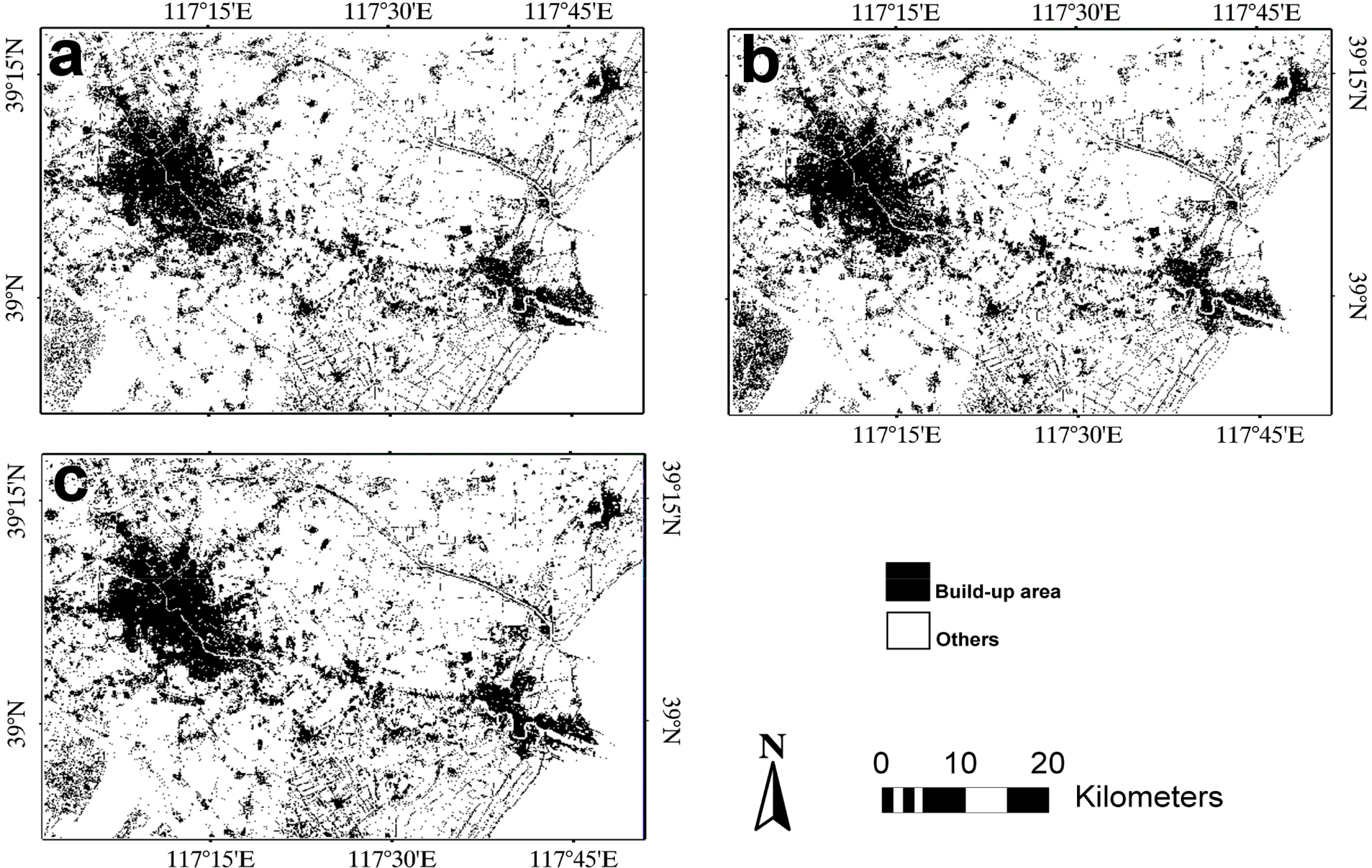
Figures 7 and 8 show the four selected classification results for the 1992 and 2006 images, respectively. From these figures, it is clear that the salt-and-pepper appearance was reduced in the classification results produced by the proposed methods (Figures 7c,d and 8c), compared with the results using spectral data alone (Figures 7a and 8a) and the results including GLCM texture (Figures 7b and 8b), especially in the lower right region of these images.
Figure 9 shows some portions of the classification results using different data combinations. From the figure, using spectral data alone or combining spectral data and GLCM texture, urban built-up areas were partially recognized (e.g., I-B, I-C of Figure 9). However, when spectral data and multivariate variogram texture were combined in the classification, the built-up area was more accurately extracted (e.g., I-D of Figure 9). When spectral data were used alone, some areas of water and harvested farmland were misclassified as urban built-up area (e.g., II-B, III-B of Figure 9). When GLCM texture was included in combined classification, the misclassification errors were slightly reduced (e.g., II-C, III-C of Figure 9). However, when multivariate variogram texture was included in classification, these misclassification errors were significantly reduced (e.g., II-D, III-D of Figure 9).
It is of note that there are some misclassification errors occurring at the boundaries between urban built-up area and other land cover classes in the classification result by the proposed method (e.g., III-D of Figure 9). These misclassification errors are mainly produced by the edge effect of the texture property [54]. In general, as in the first example (the Beijing case), the proposed method outperformed the use of spectral information alone and the joint use of spectral information and GLCM texture in bi-temporal images of the Tianjin area. Specifically, the proposed method significantly reduced the confusion between built-up area and water area and the confusion between built-up area and harvested farmland. These results demonstrated the effectiveness of the proposed methods in urban built-up area extraction.
5. Conclusions
Timely and accurate information about urban areas is very important for diverse applications. Due to significant spectral heterogeneity and spectral confusion with other land cover classes at 30-m resolution (e.g., Landsat TM/ETM+ data), the urban area extraction using spectral data from Landsat series data alone is a challenging task. This paper proposed a method that combines multivariate variogram texture and spectral data in urban area classification. The OCSVM classifier used in this study only requires the training samples from the target class (i.e., urban built-up area), while the traditional multi-class classifiers require training samples from all land cover classes. The proposed method was evaluated using bi-temporal Landsat TM/ETM+ images from two megacity areas. The experimental results indicated that the inclusion of multivariate variogram texture outperformed the use of spectral data alone and the inclusion of classical GLCM texture in classification. In particular, the inclusion of multivariate variogram texture with spectral angle distance achieved increases in the kappa coefficient from 4% to 9% compared to all other data combinations. The increases in the kappa coefficient are statistically significant in terms of McNemar’s test (at the 95% confidence level). The proposed method that employs multivariate texture and a one-class classifier (e.g., OCSVM) provides an effective and efficient way of extracting urban built-up area. The method can be also applicable to other relevant applications.
Acknowledgments
This work was funded by National Science Foundation of China (Grant Number 41371329). We would like to thank anonymous reviewers for their constructive comments, which greatly improved the quality of our manuscript.
Author Contributions
The main idea of extracting built-up area by multivariate texture and spectral information was proposed by Peijun Li. The experiments were carried out by Jun Zhang, who also prepared the figures. Jinfei Wang provided much in-depth analysis of the results. This manuscript was written by Jun Zhang.
Conflicts of Interest
The authors declare no conflicts of interest.
References
- Chameides, W.L.; Kasibhatla, P.S.; Yienger, J.; Levy, H. Growth of continental-scale metro-agro-plexes, regional ozone pollution, and world food production. Science 1994, 264, 74–77. [Google Scholar]
- Guindon, B.; Zhang, Y.; Dillabaugh, C. Landsat urban mapping based on a combined spectral-spatial methodology. Remote Sens. Environ. 2004, 92, 218–232. [Google Scholar]
- Small, C. A global analysis of urban reflectance. Int. J. Remote Sens. 2005, 26, 661–681. [Google Scholar]
- Griffiths, P.; Hostert, P.; Gruebner, O.; van der Linden, S. Mapping megacity growth with multi-sensor data. Remote Sens. Environ. 2010, 114, 426–439. [Google Scholar]
- Sun, Z.; Guo, H.; Li, X.; Lu, L.; Du, X. Estimating urban impervious surfaces from Landsat-5 TM imagery using multilayer perceptron neural network and support vector machine. J. Appl. Remote Sens. 2011. [Google Scholar] [CrossRef]
- Schneider, A. Monitoring land cover change in urban and pen-urban areas using dense time stacks of Landsat satellite data and a data mining approach. Remote Sens. Environ. 2012, 124, 689–704. [Google Scholar]
- Taubenböck, H.; Esch, T.; Felbier, A.; Wiesner, M.; Roth, A.; Dech, S. Monitoring urbanization in mega cities from space. Remote Sens. Environ. 2012, 117, 162–176. [Google Scholar]
- Wulder, M.A.; White, J.C.; Masek, J.G.; Dwyer, J.; Roy, D.P. Continuity of landsat observations: Short term considerations. Remote Sens. Environ. 2011, 115, 747–751. [Google Scholar]
- Small, C.; Lu, J.W.T. Estimation and vicarious validation of urban vegetation abundance by spectral mixture analysis. Remote Sens. Environ. 2006, 100, 441–456. [Google Scholar]
- Zha, Y.; Gao, J.; Ni, S. Use of normalized difference built-up index in automatically mapping urban areas from TM imagery. Int. J. Remote Sens. 2003, 24, 583–594. [Google Scholar]
- Xu, H. Extraction of urban built-up land features from landsat imagery using a thematic-oriented index combination technique. Photogramm. Eng. Remote Sens. 2007, 73, 1381–1391. [Google Scholar]
- Pesaresi, M.; Gerhardinger, A.; Kayitakire, F. A robust built-up area presence index by anisotropic rotation-invariant textural measure. IEEE J. Sel. Top. Appl. Earth Observ. Remote Sens. 2008, 1, 180–192. [Google Scholar]
- Xu, H. A new index for delineating built-up land features in satellite imagery. Int. J. Remote Sens. 2008, 29, 4269–4276. [Google Scholar]
- Pesaresi, M.; Gerhardinger, A. Improved textural built-up presence index for automatic recognition of human settlements in arid regions with scattered vegetation. IEEE J. Sel. Top. Appl. Earth Observ. Remote Sens. 2011, 4, 16–26. [Google Scholar]
- Deng, C.; Wu, C. BCI: A biophysical composition index for remote sensing of urban environments. Remote Sens. Environ. 2012, 127, 247–259. [Google Scholar]
- Weng, Q. Remote sensing of impervious surfaces in the urban areas: Requirements, methods, and trends. Remote Sens. Environ. 2012, 117, 34–49. [Google Scholar]
- Zhang, Q.; Wang, J.; Peng, X.; Gong, P.; Shi, P. Urban built-up land change detection with road density and spectral information from multi-temporal Landsat TM data. Int. J. Remote Sens. 2002, 23, 3057–3078. [Google Scholar]
- He, C.; Wei, A.; Shi, P.; Zhang, Q.; Zhao, Y. Detecting land-use/land-cover change in rural–urban fringe areas using extended change-vector analysis. Int. J. Appl. Earth Observ. Geoinf. 2011, 13, 572–585. [Google Scholar]
- Lyons, M.B.; Phinn, S.R.; Roelfsema, C.M. Long term land cover and seagrass mapping using Landsat and object-based image analysis from 1972 to 2010 in the coastal environment of South East Queensland, Australia. ISPRS J. Photogramm. Remote Sens. 2012, 71, 34–46. [Google Scholar]
- Haralick, R.M.; Karthikeyan, S.; Dinstein, I.H. Textural features for image classification. IEEE Trans. Syst. Man Cybernet. 1973, 6, 610–621. [Google Scholar]
- Chica-Olmo, M.; Abarca-Hernandez, F. Computing geostatistical image texture for remotely sensed data classification. Comput. Geosci. 2000, 26, 373–383. [Google Scholar]
- Wentz, E.A.; Stefanov, W.L.; Gries, C.; Hope, D. Land use and land cover mapping from diverse data sources for an arid urban environments. Comput. Environ. Urban Syst. 2006, 30, 320–346. [Google Scholar]
- Leinenkugel, P.; Esch, T.; Kuenzer, C. Settlement detection and impervious surface estimation in the Mekong delta using optical and SAR remote sensing data. Remote Sens. Environ. 2011, 115, 3007–3019. [Google Scholar]
- Bagan, H.; Yamagata, Y. Landsat analysis of urban growth: How Tokyo became the world’s largest megacity during the last 40 years. Remote Sens. Environ. 2012, 127, 210–222. [Google Scholar]
- Huang, B.; Zhang, H.; Yu, L. Improving Landsat ETM Plus urban area mapping via spatial and angular fusion with MISR multi-angle observations. IEEE J. Sel. Top. Appl. Earth Observ. Remote Sens. 2012, 5, 101–109. [Google Scholar]
- Zhu, Z.; Woodcock, C.E.; Rogan, J.; Kellndorfer, J. Assessment of spectral, polarimetric, temporal, and spatial dimensions for urban and peri-urban land cover classification using Landsat and SAR data. Remote Sens. Environ. 2012, 117, 72–82. [Google Scholar]
- Kenduiywo, B.K.; Tolpekin, V.A.; Stein, A. Detection of built-up area in optical and synthetic aperture radar images using conditional random fields. J. Appl. Remote Sens. 2014. [Google Scholar] [CrossRef]
- Karathanassi, V.; Iossifidis, C.; Rokos, D. A texture-based classification method for classifying built areas according to their density. Int. J. Remote Sens. 2000, 21, 1807–1823. [Google Scholar]
- Stefanov, W.L.; Ramsey, M.S.; Christensen, P.R. Monitoring urban land cover change: An expert system approach to land cover classification of semiarid to arid urban centers. Remote Sens. Environ. 2001, 77, 173–185. [Google Scholar]
- Dekker, R.J. Texture analysis and classification of ERS SAR images for map updating of urban areas in the Netherlands. IEEE Trans. Geosci. Remote Sens. 2003, 41, 1950–1958. [Google Scholar]
- Li, P.; Cheng, T.; Guo, J. Multivariate image texture by multivariate variogram for multispectral image classification. Photogramm. Eng. Remote Sens. 2009, 75, 147–157. [Google Scholar]
- Li, P.; Yu, H.; Cheng, T. Lithologic mapping using ASTER imagery and multivariate texture. Can. J. Remote Sens. 2009, 35, S117–S125. [Google Scholar]
- Li, P.; Xu, H.; Guo, J. Urban building damage detection from very high resolution imagery using OCSVM and spatial features. Int. J. Remote Sens. 2010, 31, 3393–3409. [Google Scholar]
- Li, P.; Xu, H.; Song, B. A novel method for urban road damage detection using very high resolution satellite imagery and road map. Photogramm. Eng. Remote Sens. 2011, 77, 1057–1066. [Google Scholar]
- Sohn, Y.S.; Moran, E.; Gurri, F. Deforestation in north-central Yucatan (1985–1995): Mapping secondary succession of forest and agricultural land use in sotuta using the cosine of the angle concept. Photogramm. Eng. Remote Sens. 1999, 65, 947–958. [Google Scholar]
- Guo, L.J.; Moore, J.M. Cloud-shadow suppression technique for enhancement of airborne thematic mapper imagery. Photogramm. Eng. Remote Sens. 1993, 59, 1287–1291. [Google Scholar]
- Kruse, F.A.; Lefkoff, A.B.; Boardman, J.W.; Heidebrecht, K.B.; Shapiro, A.T.; Barloon, P.J.; Goetz, A.F.H. The spectral image-processing system (SIPS)-interactive visualization and analysis of imaging spectrometer data. Remote Sens. Environ. 1993, 44, 145–163. [Google Scholar]
- Lu, D.; Hetrick, S.; Moran, E. Land cover classification in a complex urban-rural landscape with Quickbird imagery. Photogramm. Eng. Remote Sens. 2010, 76, 1159–1168. [Google Scholar]
- Pouch, G.W.; Campagna, D.J. Hyperspherical direction cosine transformation for separation of spectral and illumination information in digital scanner data. Photogramm. Eng. Remote Sens. 1990, 56, 475–479. [Google Scholar]
- Bourgault, G.; Marcotte, D. Multivariable variogram and its application to the linear-model of coregionalization. Math. Geol. 1991, 23, 899–928. [Google Scholar]
- Ramstein, G.; Raffy, M. Analysis of the structure of radiometric remotely-sensed images. Int. J. Remote Sens. 1989, 10, 1049–1073. [Google Scholar]
- Murphy, R.J.; Monteiro, S.T.; Schneider, S. Evaluating classification techniques for mapping vertical geology using field-based hyperspectral sensors. IEEE Trans. Geosci. Remote Sens. 2012, 50, 3066–3080. [Google Scholar]
- Lark, R.M. Geostatistical description of texture on an aerial photograph for discriminating classes of land cover. Int. J. Remote Sens. 1996, 17, 2115–2133. [Google Scholar]
- Ferro, C.J.S.; Warner, T.A. Scale and texture in digital image classification. Photogramm. Eng. Remote Sens. 2002, 68, 51–63. [Google Scholar]
- Mather, P.; Tso, B. Classification Methods for Remotely Sensed Data; CRC Press: Boca Raton, FL, USA, 2003. [Google Scholar]
- Tax, D.M.; Duin, R.P. Combining one-class classifiers. In Multiple Classifier Systems; Springer-Berlin: Heidelberg, Germany, 2001; pp. 299–308. [Google Scholar]
- Sanchez-Hernandez, C.; Boyd, D.S.; Foody, G.M. One-class classification for mapping a specific land-cover class: SVDD classification of fenland. IEEE Trans. Geosci. Remote Sens 2007, 45, 1061–1073. [Google Scholar]
- Guo, Q.; Kelly, M.; Graham, C.H. Support vector machines for predicting distribution of Sudden Oak Death in California. Ecol. Modell 2005, 182, 75–90. [Google Scholar]
- Congalton, R.G. A review of assessing the accuracy of classifications of remotely sensed data. Remote Sens. Environ. 1991, 37, 35–46. [Google Scholar]
- Smits, P.C.; Dellepiane, S.G.; Schowengerdt, R.A. Quality assessment of image classification algorithms for land-cover mapping: A review and a proposal for a cost-based approach. Int. J. Remote Sens. 1999, 20, 1461–1486. [Google Scholar]
- Foody, G.M. Thematic map comparison: Evaluating the statistical significance of differences in classification accuracy. Photogramm. Eng. Remote Sens. 2004, 70, 627–633. [Google Scholar]
- Song, C.; Woodcock, C.E.; Seto, K.C.; Lenney, M.P.; Macomber, S.A. Classification and change detection using Landsat TM data: When and how to correct atmospheric effects? Remote Sens. Environ. 2001, 75, 230–244. [Google Scholar]
- Marceau, D.J.; Howarth, P.J.; Dubois, J.M.M.; Gratton, D.J. Evaluation of the gray-level cooccurrence matrix-method for land-cover classification using SPOT imagery. IEEE Trans. Geosci. Remote Sens. 1990, 28, 513–519. [Google Scholar]
- Maillard, P. Comparing texture analysis methods through classification. Photogramm. Eng. Remote Sens. 2003, 69, 357–367. [Google Scholar]


| Training Samples | Test Samples | ||
|---|---|---|---|
| Built-Up | Built-Up | Non-Built-Up | |
| Beijing | |||
| 1995 image | 17,703 | 18,861 | 25,608 |
| 2005 image | 13,624 | 17,608 | 22,522 |
| Tianjin | |||
| 1992 image | 7717 | 10,220 | 18,547 |
| 2006 image | 7154 | 13,332 | 17,280 |
| Data Combinations | OA | Kappa | Built-Up Class | Non-Built-Up Class | ||
|---|---|---|---|---|---|---|
| PA | UA | PA | UA | |||
| Spectral + MV3_1 (Eu) | 90.90 | 81.61 | 91.97 | 87.85 | 90.06 | 93.48 |
| Spectral + MV5_1 (Eu) | 91.23 | 82.23 | 91.15 | 89.10 | 91.28 | 92.96 |
| Spectral + MV7_1 (Eu) | 91.68 | 83.05 | 89.07 | 91.72 | 93.72 | 91.64 |
| Spectral + MV9_1 (Eu) | 91.58 | 82.84 | 88.57 | 91.95 | 93.94 | 91.31 |
| Spectral + MV3_1 (Ma) | 90.70 | 81.04 | 87.43 | 91.02 | 93.26 | 90.47 |
| Spectral + MV5_1 (Ma) | 90.52 | 80.84 | 91.27 | 87.64 | 89.93 | 92.95 |
| Spectral + MV7_1 (Ma) | 91.56 | 82.91 | 91.36 | 89.62 | 91.72 | 93.14 |
| Spectral + MV9_1 (Ma) | 91.68 | 83.11 | 90.54 | 90.50 | 92.57 | 92.60 |
| Spectral + MV3_1 (Sa) | 91.78 | 83.43 | 93.87 | 88.16 | 90.15 | 94.95 |
| Spectral + MV5_1 (Sa) | 92.15 | 84.14 | 93.08 | 89.46 | 91.43 | 94.42 |
| Spectral + MV7_1 (Sa) | 92.35 | 84.49 | 91.87 | 90.81 | 92.73 | 93.58 |
| Spectral + MV9_1 (Sa) | 92.31 | 84.43 | 92.54 | 90.19 | 92.13 | 94.04 |
OA: overall accuracy; PA: producer’s accuracy; UA: user’s accuracy; spectral: six TM bands; MVw_1: multivariate variogram texture with a window size of w × w pixels and a lag distance of one pixel; Eu: Euclidean distance; Ma: Mahalanobis distance; Sa: Spectral angle distance.
| Data Combinations | OA | Kappa | Built-Up Class | |
|---|---|---|---|---|
| PA | UA | |||
| Spectral + Var | 88.75 | 77.47 | 93.71 | 82.88 |
| Spectral + Con | 89.74 | 79.37 | 92.95 | 85.05 |
| Spectral + SM | 89.56 | 79.03 | 93.11 | 84.64 |
| Spectral + Hom | 90.12 | 80.15 | 93.71 | 85.23 |
| Spectral + Dis | 90.64 | 80.96 | 88.62 | 89.90 |
| Spectral + Dis (Red) | 89.09 | 77.86 | 87.90 | 87.32 |
OA: overall accuracy; PA: producer’s accuracy; UA: user’s accuracy; spectral: six TM bands; V: variance texture; C: contrast texture; SM: second moment texture; Hom: homogeneity texture; Dis: dissimilarity texture; Dis (Red): dissimilarity texture calculated from the red band. Textures that do not mention the band were calculated from the NIR band.
| Data Combinations | OA | Kappa | Built-Up Class | Non-Built-Up Class | ||
|---|---|---|---|---|---|---|
| PA | UA | PA | UA | |||
| 1995 | ||||||
| Spectral | 89.20 | 77.96 | 88.29 | 86.53 | 89.87 | 91.25 |
| Spectral + GLCM_Dis | 89.73 | 78.98 | 87.92 | 87.88 | 91.07 | 91.10 |
| Spectral + MV_Eu | 89.82 | 79.11 | 87.08 | 88.70 | 91.83 | 90.61 |
| Spectral + MV_Ma | 89.90 | 79.29 | 87.48 | 88.56 | 91.68 | 90.86 |
| Spectral + MV_Sa | 91.72 | 83.03 | 90.04 | 90.39 | 92.95 | 92.68 |
| 2005 | ||||||
| Spectral | 88.07 | 75.82 | 87.16 | 85.87 | 88.79 | 89.84 |
| Spectral + GLCM_Dis | 90.64 | 80.96 | 88.62 | 89.90 | 92.21 | 91.20 |
| Spectral + MV_Eu | 91.68 | 83.05 | 89.07 | 91.72 | 93.72 | 91.64 |
| Spectral + MV_Ma | 91.56 | 82.91 | 91.36 | 89.62 | 91.72 | 93.14 |
| Spectral + MV_Sa | 92.35 | 84.49 | 91.87 | 90.81 | 92.73 | 93.58 |
OA: overall accuracy; PA: producer’s accuracy; UA: user’s accuracy; spectral: spectral data; GLCM_Dis: dissimilarity texture from GLCM; MV_Eu: multivariate variogram texture with Euclidean distance; MV_Ma: multivariate variogram texture with Mahalanobis distance; MV_Sa: multivariate variogram texture with spectral angle distance.
| Spectral | Spectral + GLCM_Dis | Spectral + MV_Eu | Spectral + MV_Ma | Spectra + MV_Sa | |
|---|---|---|---|---|---|
| 1995 | |||||
| Spectral | \ | S | S | S | S |
| Spectral + GLCM_Dis | 2.4386 | \ | NS | NS | S |
| Spectral + MV_Eu | 2.8265 | 0.3880 | \ | NS | S |
| Spectral + MV_Ma | 3.2054 | 0.7671 | 0.3791 | \ | S |
| Spectral + MV_Sa | 12.1263 | 9.7105 | 9.3136 | 8.9359 | \ |
| 2005 | |||||
| Spectral | \ | S | S | S | S |
| Spectral + GLCM_Dis | 11.1329 | \ | S | S | S |
| Spectral + MV_Eu | 16.0409 | 4.9499 | \ | NS | S |
| Spectral + MV_Ma | 15.4989 | 4.4018 | 0.5487 | \ | S |
| Spectral + MV_Sa | 19.3730 | 8.3273 | 3.3851 | 3.9334 | \ |
S: significant; NS: not significant.
| Data Combinations | OA | Kappa | Built-Up Class | Non-Built-Up Class | ||
|---|---|---|---|---|---|---|
| PA | UA | PA | UA | |||
| 1992 | ||||||
| Spectral | 86.54 | 70.64 | 81.24 | 80.94 | 89.46 | 89.64 |
| Spectral + GLCM_Dis | 86.86 | 71.37 | 81.92 | 81.25 | 89.58 | 89.99 |
| Spectral + MV_Eu | 89.31 | 76.70 | 85.23 | 84.76 | 91.56 | 91.84 |
| Spectral + MV_Ma | 88.20 | 74.15 | 82.58 | 83.95 | 91.30 | 90.49 |
| Spectral + MV_Sa | 90.72 | 79.67 | 86.19 | 87.50 | 93.21 | 92.45 |
| 2006 | ||||||
| Spectral | 85.21 | 69.92 | 82.97 | 83.06 | 86.94 | 86.87 |
| Spectral + GLCM_Dis | 86.07 | 71.60 | 83.00 | 84.70 | 88.44 | 87.08 |
| Spectral + MV_Eu | 86.72 | 72.96 | 84.32 | 85.05 | 88.56 | 87.98 |
| Spectral + MV_Ma | 86.64 | 72.83 | 84.66 | 84.67 | 88.17 | 88.17 |
| Spectral + MV_Sa | 89.54 | 78.65 | 86.49 | 89.16 | 91.89 | 89.81 |
OA: overall accuracy; PA: producer’s accuracy; UA: user’s accuracy; spectral: spectral data; GLCM_Dis: dissimilarity texture from GLCM; MV_Eu: multivariate variogram texture with Euclidean distance; MV_Ma: multivariate variogram texture with Mahalanobis distance; MV_Sa: multivariate variogram texture with spectral angle distance.
| Spectral | Spectral + GLCM_Dis | Spectral + MV_Eu | Spectral + MV_Ma | Spectral + MV_Sa | |
|---|---|---|---|---|---|
| 1992 | |||||
| Spectral | \ | NS | S | S | S |
| Spectral + GLCM_Dis | 1.0517 | \ | S | S | S |
| Spectral + MV_Eu | 9.5622 | 8.5150 | \ | S | S |
| Spectral + MV_Ma | 5.6076 | 4.5573 | 3.9662 | \ | S |
| Spectral + MV_Sa | 14.8610 | 13.8211 | 5.3433 | 9.2973 | \ |
| 2006 | |||||
| Spectral | \ | S | S | S | S |
| Spectral + GLCM_Dis | 2.7942 | \ | S | NS | S |
| Spectral + MV_Eu | 4.9731 | 2.1802 | \ | NS | S |
| Spectral + MV_Ma | 4.7187 | 1.9256 | 0.2547 | \ | S |
| Spectral + MV_Sa | 15.0591 | 12.2892 | 10.1222 | 10.3755 | \ |
S: significant; NS: not significant.
© 2014 by the authors; licensee MDPI, Basel, Switzerland This article is an open access article distributed under the terms and conditions of the Creative Commons Attribution license (http://creativecommons.org/licenses/by/3.0/).
Share and Cite
Zhang, J.; Li, P.; Wang, J. Urban Built-Up Area Extraction from Landsat TM/ETM+ Images Using Spectral Information and Multivariate Texture. Remote Sens. 2014, 6, 7339-7359. https://0-doi-org.brum.beds.ac.uk/10.3390/rs6087339
Zhang J, Li P, Wang J. Urban Built-Up Area Extraction from Landsat TM/ETM+ Images Using Spectral Information and Multivariate Texture. Remote Sensing. 2014; 6(8):7339-7359. https://0-doi-org.brum.beds.ac.uk/10.3390/rs6087339
Chicago/Turabian StyleZhang, Jun, Peijun Li, and Jinfei Wang. 2014. "Urban Built-Up Area Extraction from Landsat TM/ETM+ Images Using Spectral Information and Multivariate Texture" Remote Sensing 6, no. 8: 7339-7359. https://0-doi-org.brum.beds.ac.uk/10.3390/rs6087339