Evaluating MERIS-Based Aquatic Vegetation Mapping in Lake Victoria

Abstract
: Delineation of aquatic plants and estimation of its surface extent are crucial to the efficient control of its proliferation, and this information can be derived accurately with fine resolution remote sensing products. However, small swath and low observation frequency associated with them may be prohibitive for application to large water bodies with rapid proliferation and dynamic floating aquatic plants. The information can be derived from products with large swath and high observation frequency, but with coarse resolution; and the quality of so derived information must be eventually assessed using finer resolution data. In this study, we evaluate two methods: Normalized Difference Vegetation Index (NDVI) slicing and maximum likelihood in terms of delineation; and two methods: Gutman and Ignatov’s NDVI-based fractional cover retrieval and linear spectral unmixing in terms of area estimation of aquatic plants from 300 m Medium Resolution Imaging Spectrometer (MERIS) data, using as reference results obtained with 30 m Landsat-7 ETM+. Our results show for delineation, that maximum likelihood with an average classification accuracy of 80% is better than NDVI slicing at 75%, both methods showing larger errors over sparse vegetation. In area estimation, we found that Gutman and Ignatov’s method and spectral unmixing produce almost the same root mean square (RMS) error of about 0.10, but the former shows larger errors of about 0.15 over sparse vegetation while the latter remains invariant. Where an endmember spectral library is available, we recommend the spectral unmixing approach to estimate extent of vegetation with coarse resolution data, as its performance is relatively invariant to the fragmentation of aquatic vegetation cover.
1. Introduction
Aquatic weed infestation is one of the major environmental challenges globally. The weeds, which mostly comprise water hyacinth and hippo-grass, are associated with many adverse effects. Continuous observation and monitoring of their proliferation is essential for proper lake management and weed control [1]. Remote sensing information has increasingly become essential for water resource management. It is a powerful tool for studying large scale phenomena in aquatic vegetation communities, and is capable of delivering timely information unmatched by any other surveying technique [2]. High resolution data such as those acquired by IKONOS and Korea Multi-Purpose Satellite (KOMPSAT) satellites provide detailed information but are associated with low observation frequency and small swath, and their cost may be prohibitively expensive for large area assessments [3]. A common remote sensing practice is to mosaic spatially adjacent images that are acquired within a short temporal range to produce extensive cover maps. Rapid proliferation and the dynamic nature of floating aquatic vegetation have the implication that mosaicking is not suitable for aquatic environments with freely floating vegetation. Coarse resolution products such as Medium Resolution Imaging Spectrometer (MERIS) and MODIS provide a wider view and higher data frequency at the expense of spatial details. Because of this inherent trade-off, it may be appropriate to use coarse resolution data for continuous frequent observation of aquatic vegetation, and occasionally use the high resolution data to assess the quality of derived information.
Frequent and accurate monitoring of aquatic vegetation is not only essential in providing reliable and timely information to the lake management authorities for sustained water resource management [4], but also in improving the quality of related studies which rely on this information for their analyses. For example a study to evaluate the effect of nutrient influx on vegetation proliferation would require adequately accurate information on the extent and location of aquatic plants. Assessing the accuracy of remotely derived information allows users to ascertain their reliability, and it is a means through which the producers communicate product limitations to users, leading to appropriate use of the information [5]. According to [6], accuracy assessment of remote sensing map products has evolved in four developmental stages. It started with visual assessment of images to determine whether the classification results were good or not. It improved to the stage where an overall non-site-specific percentage accuracy was provided, and further to a site-specific accuracy assessment. Finally, a more detailed analysis of the site-specific accuracy assessments emerged, for example the use of error/confusion matrix and kappa coefficients. Error matrix has become one of the most commonly used method of classification accuracy assessment, with several applications in land use/land cover mapping, for example [7] and [8]. This method requires manual identification of reference sites/pixels from homogeneous surfaces, which are assumed to represent pure feature classes (endmembers) [9]. Error matrix also allows the use of “Pareto Boundary” analysis of the trade-off between commission and omission error, in order to determine the optimal classification performance that can be obtained for a specific low resolution data.
Several algorithms have been developed for the remote retrieval of biophysical characteristics of vegetation. The authors of [1] used an unsupervised clustering technique with thresholds based on a “wetness index”, to identify water hyacinth and water hyacinth-free areas in Lake Victoria. The authors of [10] applied Minimum Distance—a simple parametric classification algorithm to identify floating vegetation areas, before applying a spectral linear mixture model—a sub-pixel analysis to discriminate different vegetation species according to the weed spectral behaviour. The most widely used method, however, is the mathematical combination of visible and near-infrared reflectance bands in the form of spectral vegetation indices [11]. Vegetation indices are widely used because of their computational simplicity. Many studies on Lake Victoria have used vegetation indices, for example, [12] used NDVI to investigate the dependency of hyacinth biomass production on nutrients levels. In [13], the authors used a time-series of NDVI to evaluate the link between the occurrence of El Nino events in East Africa and water hyacinth blooms in Winam Gulf section of Lake Victoria. The authors of [14] used NDVI and several of its derivatives to monitor Lake Victoria’s water level and drought conditions. More recently [15] used NDVI to map vegetation distribution in the lake, and to develop a floating vegetation index for quantifying its surface extent.
Vegetation cover estimates obtained with remote sensing methods can provide useful decision support information required for the control of aquatic plants proliferation. This information can only be useful if the practitioners have a way of ascertaining its accuracy. Little information is available on the accuracy of aquatic vegetation cover estimates derived at coarse resolution. The accuracy of a method in detection of terrestrial vegetation and aquatic vegetation may be different because of the difference in backgrounds. Water, which forms the background to aquatic vegetation, has a stronger absorption of electromagnetic radiation than soil. Further, the dynamic nature of the floating aquatic vegetation introduces a unique case to the evaluation of detection accuracy of aquatic vegetation. Floating vegetation is carried away by tides and wind, making it difficult to identify sampling sites where manual vegetation cover estimates can be made. Unlike in the case of terrestrial vegetation where the target is stationary, it is technically challenging to collect reference in situ measurements. A viable alternative is to use as reference results obtained with finer resolution remote sensing products. In addition, the reference image must have its acquisition time as close as possible, ideally in the order of minutes, to that of the classified image. Obtaining such pair of data is perhaps the biggest challenge in the assessment of floating aquatic vegetation classifications.
Our objective is to evaluate the performance of algorithms commonly used to monitor aquatic plants in extensive water bodies, in terms of their accuracy in detecting aquatic plants from coarse resolution remote sensing data—in this case the 300 m resolution MERIS data. MERIS sensor ended data acquisition in March 2013, but its products are good test data for the anticipated Sentinel 2/3 products. In terms of delineation, we evaluate two methods: NDVI slicing—with special focus on the empirical slicing proposed by [15], and maximum likelihood classifier. In terms of area estimation, we evaluate two methods: NDVI-based fractional cover retrieval model proposed by [16], and linear spectral unmixing (LSU)—which is a form of spectral mixture analysis. We also aim at assessing the suitability of using higher resolution data as reference in assessing the quality of aquatic vegetation cover information obtained with coarse resolution products.
2. Study Area
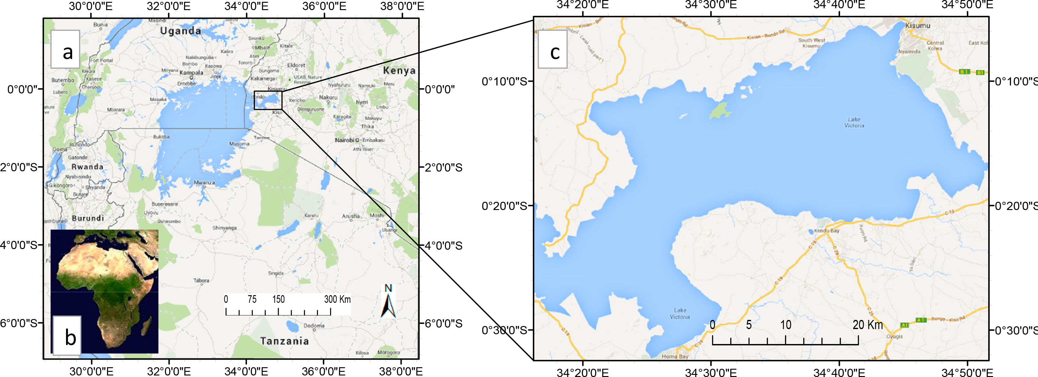
Our study area is the Winam Gulf section of Lake Victoria. Lake Victoria is a large fresh water body in East Africa. It stretches 412 km from north to south between 0°30′N and 3°12′S and 355 km from west to east between 31°37′E and 34°53′E. The lake, which is the largest of all African lakes, is also the second largest freshwater body in the world by area, with an extensive surface area of 68,800 km2. Figure 1 shows the geographic location of Lake Victoria.
We focus on the Winam Gulf because this almost enclosed shallow section of the lake is more vulnerable to vegetation invasion perhaps due to high levels of eutrophication. Earlier work of [15] show that vegetation proliferation is preceded by about two months by high levels of water quality indicators such as total suspended matter (TSM) and phytoplankton measured as a Chlorophyll-a (Chl-a) index. The most prevalent of these invasive weeds include the non-native water hyacinth and hippo-grass. The weeds are associated with many adverse effects which include obstruction to fishing, navigation and irrigation, interference with the aquatic biodiversity [17,18], water quality deterioration and a general risk to public health [19]. The lake is an important economic resource to the three riparian countries, Kenya, Tanzania and Uganda, through fishing and transport, as well as providing a livelihood for the local communities.
3. Materials and Method
3.1. Data
We use two pairs of coarse and fine resolution images, acquired almost simultaneously, to evaluate the performance of four algorithms in retrieval of aquatic vegetation cover information. MERIS (Medium Resolution Imaging Spectrometer) image in its full resolution mode (MERIS FR) has a spatial resolution of 300 m. We use as reference the results obtained with Landsat-7 ETM+ imagery at 30 m spatial resolution. Due to the dynamic nature of floating aquatic vegetation, the key consideration in selecting data for use in assessing the classification accuracy of aquatic vegetation is the temporal proximity of the image pair. During a field survey, it was estimated to take about an hour for a floating vegetation mat to move across a length approximately equal to the size of a MERIS pixel (300 m). Allowing vegetation displacement to a maximum of 0.25 of the pixel, then the interval between the acquisitions of the image pair should not be longer than 15 min. For the period 2003–2012, the entire lifetime of MERIS sensor, there are just seven scenes of Winam Gulf whose acquisition time coincides with those of ETM+, with acquisition intervals of the image pairs ranging from two to fifteen minutes. We selected two of these image pairs for our analysis, and their specifications are summarised in Table 1. The choice of these image pairs is based primarily on the short acquisition interval, and secondarily on the amount and distribution of aquatic vegetation in the images. Central acquisition time for each image is indicated. Since the image pairs were acquired almost simultaneously, we assume similar conditions of cloud, haze and water surface roughness (due to wind conditions). One of the greatest confounding factors limiting the quantity and accuracy of remotely sensed data from water bodies is sun glint, the specular reflection of directly transmitted sunlight from the upper side of the air-water interface [20]. Sun glint is a function of the state of the water surface (surface roughness), sun position and satellite viewing angle. Sun zeniths of 30°–60° degrees are optimal for minimizing sunglint [21]. Sun zenith angles are respectively 34.6° and 35.4° for MERIS and ETM+. The range of sensor viewing angles across the study area is indicated for each image. Since the radiance received by sensor is inversely proportional to the cosine of the sensor view angle, then sunglint effect on the images is negligible.
3.2. Pre-Processing
Before using the satellite data, we convert the sensor radiance values into reflectance values and perform atmospheric corrections as here described. Atmospheric corrections of MERIS data were performed using SMAC Processor 1.5.203 (a Simplified Method for Atmospheric Corrections of satellite measurements) [22], incorporated in the software package BEAM (Basic ERS and Envisat (A) ATSR and MERIS Toolbox). It is a semi-empirical approximation of the radiative transfer in the atmosphere which takes into account the attenuation due to atmospheric absorption and radiance of the scattered skylight. We used FLAASH (Fast Line-of-sight Atmospheric Analysis of Spectral Hypercubes), an atmospheric correction code based on the MODTRAN 4 (MODerate resolution atmospheric TRANsmission) radiative transfer model, to convert Landsat-7 ETM+ sensor radiance to surface reflectance. A certain degree of geolocation errors is inevitable when dealing with multiple data sets. We co-registered the image pairs using an image to image first order polynomial transformation and nearest neighbour resampling, with RMSE = 0.0745 and RMSE = 0.1218 for image pair 1 and 2 respectively. This represents a geolocation error of about 22.35 m for image pair 1, and 36.54 m for image pair 2, which is about the pixel size of the reference image. This may have an impact on the margins of the sample areas, but minimal.
3.3. Sampling
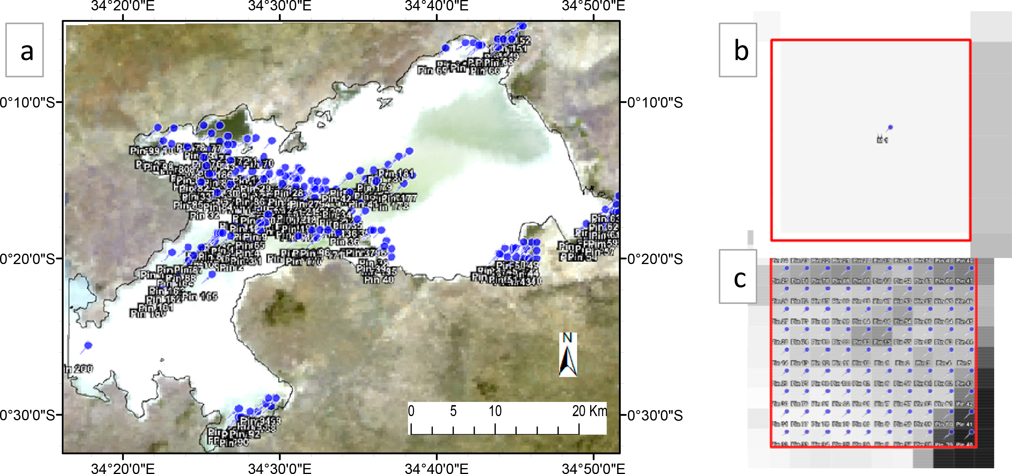
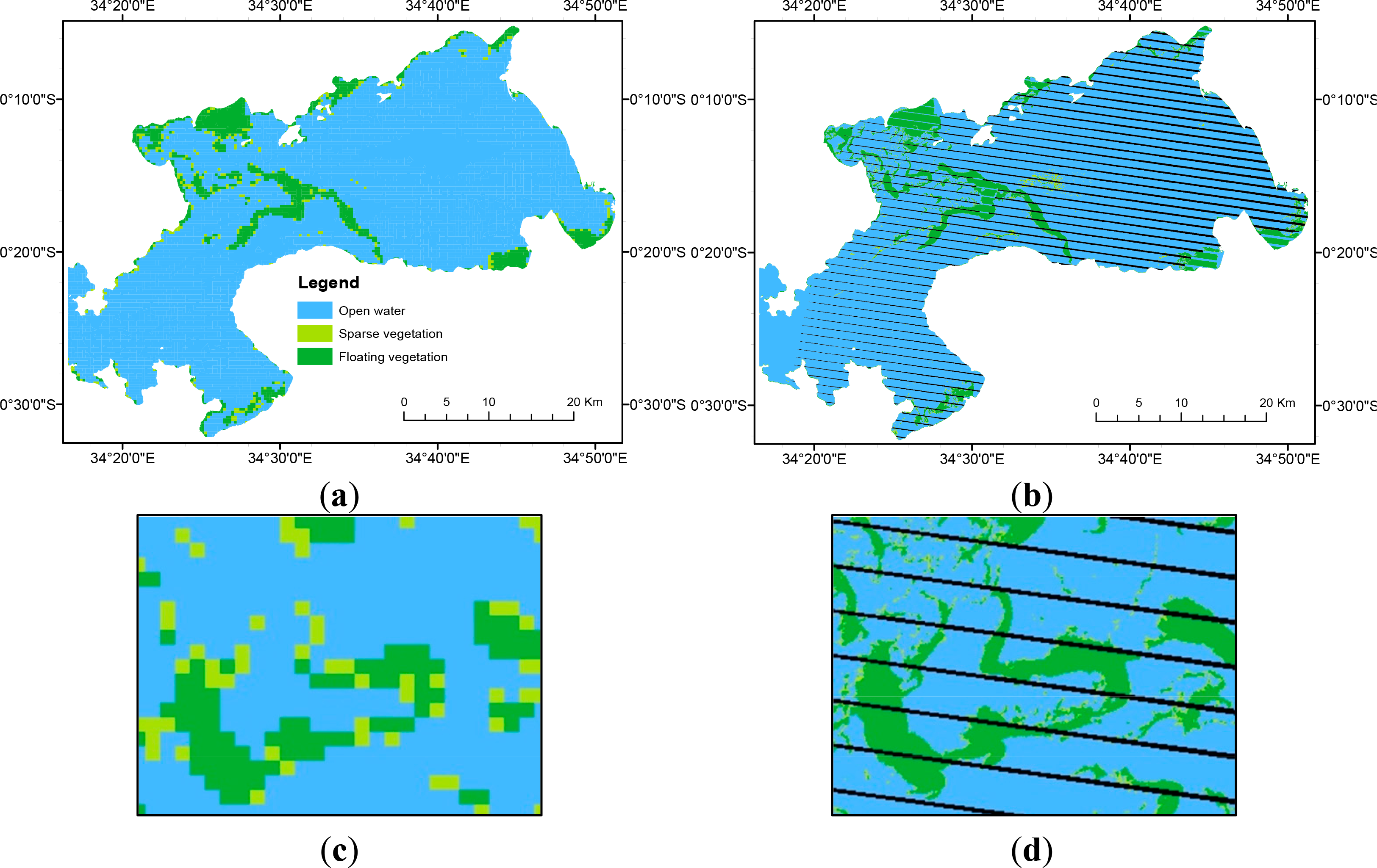
Evaluation of methods was carried out with two hundred (300 m × 300 m) samples. Each MERIS sample pixel corresponds to a square area covered by 10 × 10 ETM+ (30 m × 30 m) pixels. Sample MERIS pixels were selected such that their corresponding location in the ETM+ image would fall right in the middle of the stripes occasioned by the scan line corrector (SLC) failure in Landsat-7, so as to avoid the no-data pixels. Under these restrictive circumstances, a limited number of samples were selected. The samples were selected in Winam Gulf to include both the high and low vegetation density areas, as well as areas along the vegetation-water edges. Figure 2a shows the selected sample pixels for image pair 1; Figure 2b is a close-up (300 m × 300 m) MERIS pixel, while Figure 2c shows the corresponding one hundred (30 m × 30 m) ETM+ pixels. Although we use a shoreline derived from high resolution data to isolate our study area, we avoided samples too close to the shore, to avoid a possible confusion with terrestrial vegetation due to an imperfect shoreline.
3.4. Experimental Design
Our objective is to determine and monitor the lake area covered by aquatic vegetation: because of the size of Lake Victoria and the temporal variability of the extent of aquatic vegetation, satellite data should provide observations at daily intervals or shorter, with spatial resolution limited to 1 km or worse. We aim at determining the total lake area covered by aquatic vegetation and at delineating it.
In this study we regard MERIS as our primary source of observations and we want to assess the accuracy of both estimated total area and of the delineation of it. We used Landsat ETM+ data as a reference.
In summary we have evaluated different ways to determine the two variables of interest using the methods listed below and described in the following sections:
Delineation: slicing of NDVI, maximum likelihood classifier;
Total area: retrieval of fractional abundance from NDVI and by linear spectral un-mixing;
All four methods have been applied to MERIS data and evaluated against results obtained with ETM+. The list of image data has been given in Table 1, while the design of the evaluation experiment is given in Table 2.
3.5. Empirical Slicing of Vegetation Indices
Though many vegetation indices have been developed [23], in this study we focus on Normalized Difference Vegetation Index (NDVI) [24]. It is a dimensionless quantity which is an indicator of the greenness of vegetation, and is based on the contrast between the maximum reflection in the near infrared (ρnir) caused by leaf cellular structure and the maximum absorption in the red (ρr) due to chlorophyll pigments [25]. It is expressed as a ratio of the difference and the sum of ρnir and ρr:
NDVI is the most commonly used indicator of vegetation parameters in remotely sensed data for global vegetation mapping [25,26]. It has been applied to quantify the vegetation cover in various studies, both in terrestrial environment [27,28] as well as aquatic environment [29]. Empirical slicing of vegetation indices is commonly used to discriminate vegetation from other cover classes. The challenge, however, is the correct identification of suitable thresholds separating various feature classes in the scene. The authors of [13] applied NDVI = 0.1 as a threshold to detect presence of vegetation, while [15] estimated the aquatic vegetation cover in Lake Victoria using a three-level NDVI scale:
We give a special reference to the NDVI slicing in Equation (2) to assess accuracy of aquatic vegetation classification with NDVI slicing. While this slicing clearly provides an excellent display of the spatial distribution of vegetation in the lake as seen in [15], in this study we evaluate the impact of limiting NDVI to a few classes. NDVI was computed from Landsat-7 ETM+ using red and near infrared bands 3 and 4 centred at 660 nm and 825 nm respectively; while MERIS NDVI was computed using bands 7 and 13 centred at 664 nm and 865 nm.
3.6. Maximum Likelihood Classification
Maximum likelihood is a conventional classifier, which assigns a pixel to the class to which it most probably belongs according to a Bayesian probability function. Based on statistics (mean; variance/covariance), the probability function is calculated from the inputs for classes established from training sites. In this study, binary images consisting of water and vegetation classes were achieved by applying maximum likelihood classifier to MERIS and ETM+. The training sites for water and vegetation were obtained from the same images. This was implemented in the software package ENVI.
3.7. Estimating Vegetation Fractional Cover (fv) from NDVI
Vegetation amount is usually parameterized through the fractional area (fv) of the vegetation occupying each grid cell, which gives its horizontal density [30]. fv is sometimes estimated from vegetation indices. NDVI does not directly give fv, and some methods have been developed to derive it from vegetation indices. A commonly-used linear model for deriving fv from vegetation indices [31] is described by [16] as:
3.8. Linear Spectral Unmixing (LSU)
Linear spectral unmixing is one of the spectral mixture analysis (SMA) techniques which decompose a mixed pixel into various distinct components. It is most suitable where the spatial resolution of the satellite data is relatively coarse. It has been applied in various studies including analysis of rock and soil types [32], desert vegetation [33], land-cover changes [34], estimation of urban vegetation abundance [35], and delineating potential erosion areas in tropical watersheds [9]. Non-linear mixture models also exist [36], but linear spectral unmixing is by far the most common type of SMA, and is widely used because of its simplicity and interpretability [9]. It is a supervised classification technique which is based on the assumption that the observed reflectance of a pixel (ρk) at wavelength (k) is a linear combination of the reflectance (ρi,k) of individual class features represented in that pixel, and the contribution of each depends on its respective abundance (fi). The basic physical assumption is that there is not a significant amount of photon multiple scattering between the macroscopic materials. For a specified number of endmembers (n), linear spectral unmixing can be expressed as:
εk is the residual error. The unknown value in the expression is the fractional abundance fi and which the model estimates. We used a fully constrained model which requires that for all i, fi must sum to unity and is non-negative. The number of spectral bands in an image introduces a limitation to the number of endmembers that can be used for unmixing [37], so that it must always be less than the number of available bands in the multispectral image. The model retrieves the spectral characteristics ρi of endmembers from an input endmember spectral library.
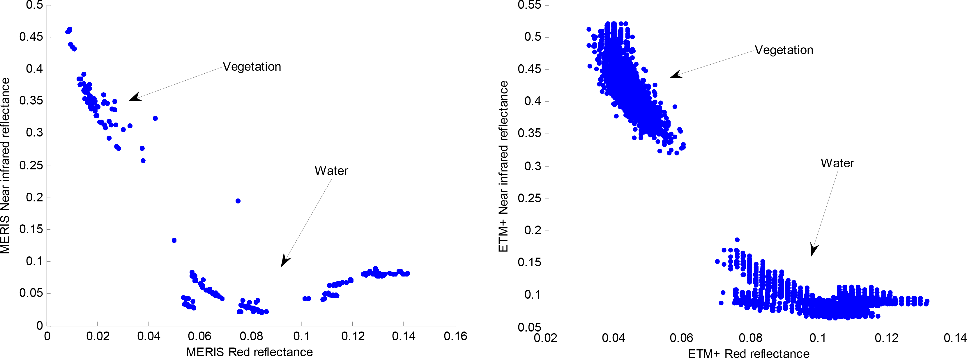
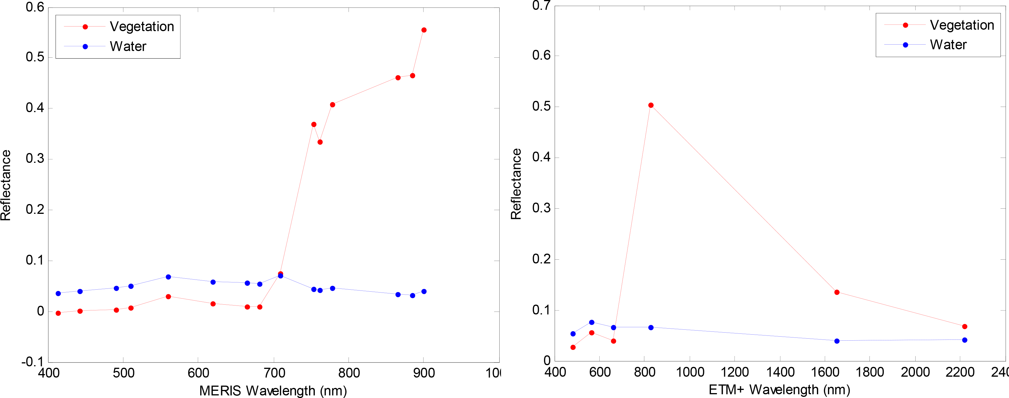
In order to build an endmember library for our study region, we first need to identify the appropriate number of endmembers. Spectral characteristics of water in the lake vary spatially according to the concentrations of dissolved or suspended sediments in it, indicating the extent of nutrient enrichment. Clearer and deeper water in the centre of the lake displays low reflectance values, while that near the shores displays generally higher reflectance values. In order to understand the spectral variability of the study area, we performed K-Means clustering [38,39], an unsupervised classification of clouds-free MERIS image whose acquisition date (15 December 2010) coincides with a field survey. K-Means is a statistical clustering method which follows the following procedure for a specified cluster number (k): (1) randomly choose k pixels whose samples define the initial cluster centres; (2) assign each pixel to the nearest cluster centre as defined by the Euclidean distance; (3) recalculate the cluster centres as the arithmetic means of all samples from all pixels in a cluster; and (4) repeat steps 2 and 3 until the convergence criterion is met. The convergence criterion is met when the maximum number of iterations specified by the user is exceeded or when the cluster centres did not change between two iterations. We begin by setting k first to 14 and specifying 30 iterations. A spectral plot of the 14 resultant classes revealed about five significantly unique classes. K-Means was repeated with k = 5, resulting in five classes; one confirmed by a field survey as vegetation and four different ‘water species’ confirmed by their relatively low reflectance values. A scatter plot of red and near infrared spectral bands for selected regions of the resulting five classes (Figure 3) showed that spectral variability among the four water classes was small with respect to the vegetation. Since vegetation was our target class, we reduced the number of endmembers to two by obtaining an average spectrum for the four water classes. Figure 3 shows good separability between vegetation and water classes, with vegetated pixels clustered at the top-left corner of the two dimensional space, due to vegetation’s strong absorption of the red and high reflection of the near infrared radiation. Water pixels are clustered at the bottom right corner, due to water’s strong absorption of the near infrared radiation.
To ensure consistency, endmember spectral libraries for MERIS and ETM+ shown in Figure 4 were compiled from the same area sampling.
We apply a fully constrained linear spectral unmixing model (Equation (4)), using as input parameters the two endmembers spectral libraries shown in Figure 4, to estimate aquatic (fv) from MERIS and ETM+ images respectively. This was implemented in the software package BEAM. The model outputs for each endmember a grey scale image, with pixel values indicating the class densities (fi) in the range of 0–1. We pick the vegetation density (fv) image for our analysis. We then assess the performance of spectral unmixing in vegetation detection using exactly the same 200 sample pixels that were used for the NDVI accuracy assessment.
4. Results and Discussion
4.1. Area-Averaging of NDVI
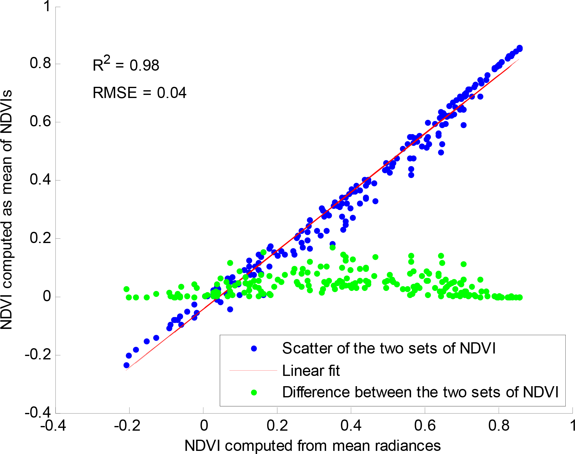
Due to non-linearity nature of NDVI, area-averaged NDVI obtained by averaging NDVIs of high resolution pixels is usually different from that obtained with averaged radiances of the high resolution pixels. Figure 5 shows a comparison of the two sets of area-averaged NDVI for 200 samples, each averaged from a hundred high resolution pixels. Even though the two sets of average NDVIs seem to compare well with R2 = 0.98 and RMSE = 0.04, variations of mean NDVI computed from the two methods can be as high as 0.17 (see the green dots in Figure 5). This difference is quite significant especially for a study where averaged NDVI is an important variable used to derive another parameter. In this study, the NDVI of a square area represented by 100 ETM+ pixels corresponding to one MERIS pixel was obtained by first averaging the reflectance of 100 ETM+ pixels in the red and near infrared, before using them to compute NDVI.
4.2. Sliced Normalized Difference Vegetation Index (NDVI)
Figure 6 shows NDVI images of the Winam Gulf section of Lake Victoria as derived from MERIS and ETM+ data. Figure 6a is MERIS NDVI while Figure 6c is ETM+ NDVI. The large green area in the centre of the lake is a floating mat of aquatic vegetation. The image shows the three classes described in Equation (2); open water (OW), sparse vegetation (SV) and floating vegetation (FV). The stripes in ETM+ image are a consequence of the SLC failure in the Landsat-7 satellite, resulting in no-data pixels. As expected, it is clear from these images that the higher resolution ETM+ (30 m) displays more vegetation cover details than MERIS (300 m), as seen from the close-up portions of the images.
Error matrices in Table 3 show the quantitative assessment of the classification accuracy of NDVI slicing. The rows show classification of the 200 MERIS sample pixels to the three classes of Equation (2); FV, SV and OW. The columns show classification of the reference pixels (ETM+) to the same classes according to Equation (2).
The diagonal matrix of the error matrix of the first image pair, Table 3(left), shows that 153 of the 200 sample pixels are correctly classified, which gives an overall classification accuracy of 76.5%. The error matrix of the second image pair, Table 3(right), shows an overall classification accuracy of 73%. In both cases, the commission and omission errors in the classification of SV are higher than those of FV and OW, indicating that major misclassifications occurred along the water-vegetation boundaries. These results seem to confirm the findings of [31], where the reported classification accuracies for NDVI of pixels along the edges of distinct endmembers were generally lower than those of non-edges. This is a common weakness to all “hard” classifiers which output discrete feature classes, and only gets worse with lower resolutions. Since NDVI slicing is heavily biased along the water-vegetation boundaries, it may have a significant impact on detection of aquatic vegetation from low resolution data. Slicing NDVI to a few levels also limits its sensitivity to vegetation density variations.
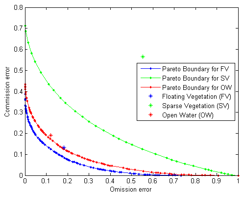
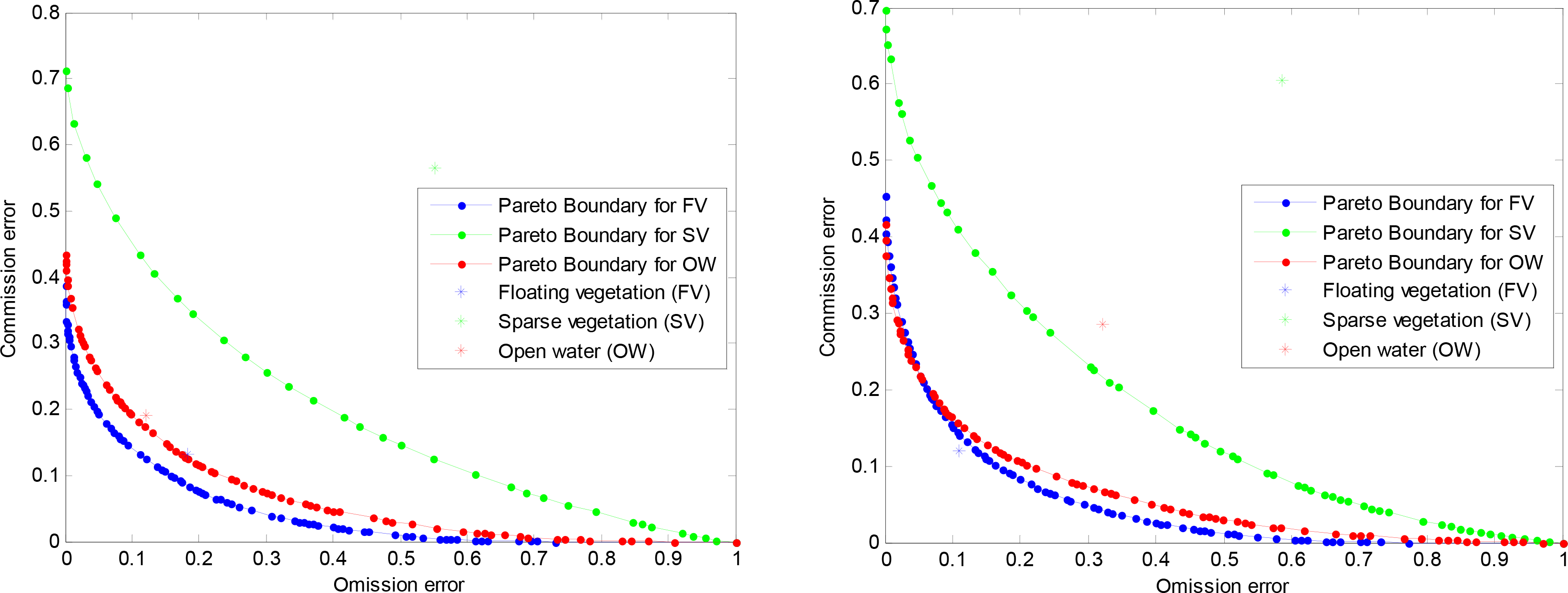
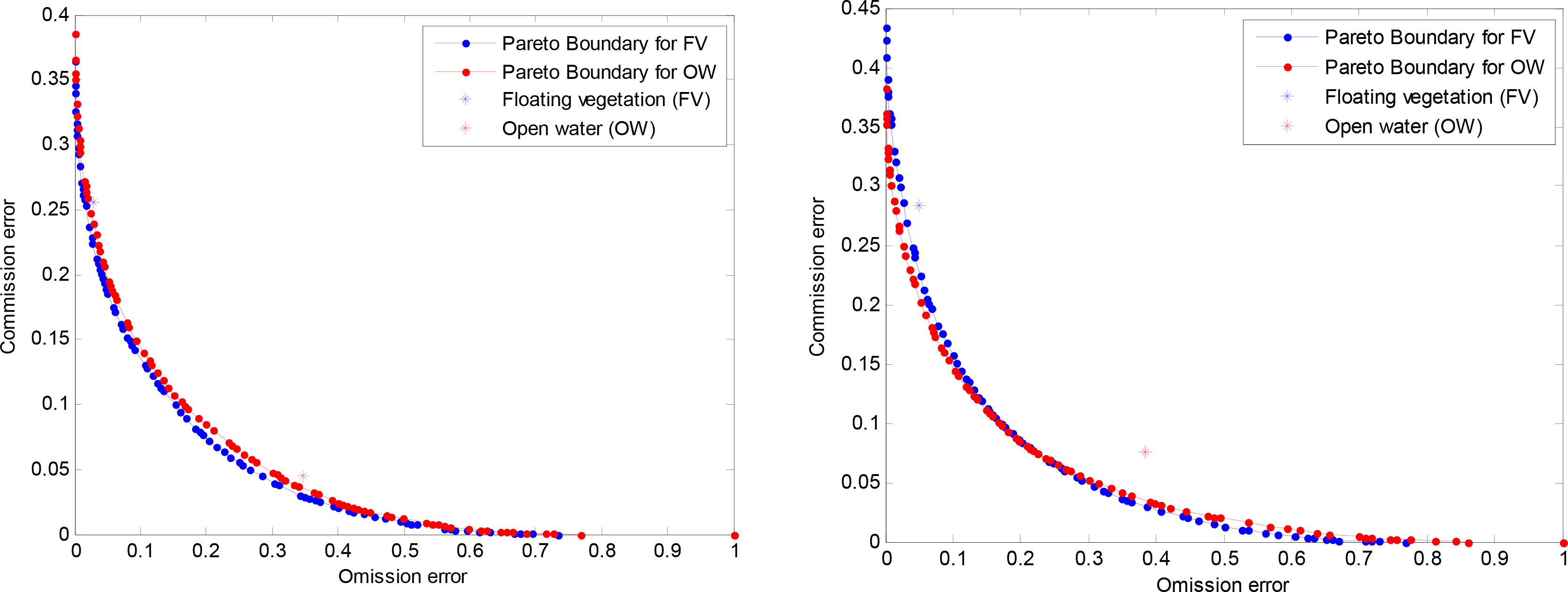
It is however known that some errors are due to the low resolution of the data rather than the weakness of the classification algorithm, a concept known as “low resolution bias” explained by [40] using Pareto Boundary. Using the Pareto Boundary, it is possible to determine the optimal classification accuracies that can be obtained by an algorithm, beyond which it is impossible to reduce the commission errors without increasing the omission errors, and vice versa. If all the pure pixels are correctly classified, then the irreducible errors are assumed to be due to the low resolution of the data. We refer readers to article [40] for a detailed description of the low resolution bias.
Figure 7 shows Pareto Boundaries for the optimal classification of floating vegetation, sparse vegetation and open water. This was obtained by setting a series of thresholds for the number of high resolution pixels of a specific class that are required to assign a low resolution pixel to that class, and computing the commission and omission errors incurred at each threshold level. Though Pareto Boundary applies only to dichotomic classifications, these results were obtained by first considering FV and collapsing SV and OW into the background, and repeating the procedure for SV and OW; resulting in three Pareto Boundaries, one for each class. Positions of the commission and omission errors obtained from the error matrix are shown in the commission error—omission error space; indicating how close the classification results are to the optimal levels.
In both image pairs, the positions of the commission and omission errors of SV are clearly farther away from their Pareto Boundaries, further confirming observations made from Table 3, that slicing of NDVI results in major misclassifications especially along the water-vegetation boundary. The radiance from this multi-class boundary received by a low resolution sensor is a combination of the spectral responses of the representative classes, and a “hard” classification of such a pixel results in high commission and omission errors.
4.3. Maximum Likelihood Classification
Error matrices in Table 4 show accuracy assessment of vegetation delineation obtained with binary Maximum Likelihood classifier for image pair 1 (left) and image pair 2 (right).
The rows show classification of MERIS sample pixels to two classes; FV and OW. The columns show classification of regions corresponding to MERIS sample pixels to two classes; FV class for regions half or more of ETM+ pixels are classified as vegetation, and OW class where less than half of ETM+ pixels are classified as vegetation. These results show an overall classification accuracy of 81.5% and 78.5% for pair 1 and pair 2 respectively. Pareto boundary analyses of the trade-off between commission and omission errors in these classifications are presented in Figure 8. In both cases, the positions of the omission and commission errors in the classification of vegetation and water are close to their respective Pareto boundaries, indicating a good performance of the classifier.
4.4. Estimating Vegetation Fractional Cover (fv) from NDVI
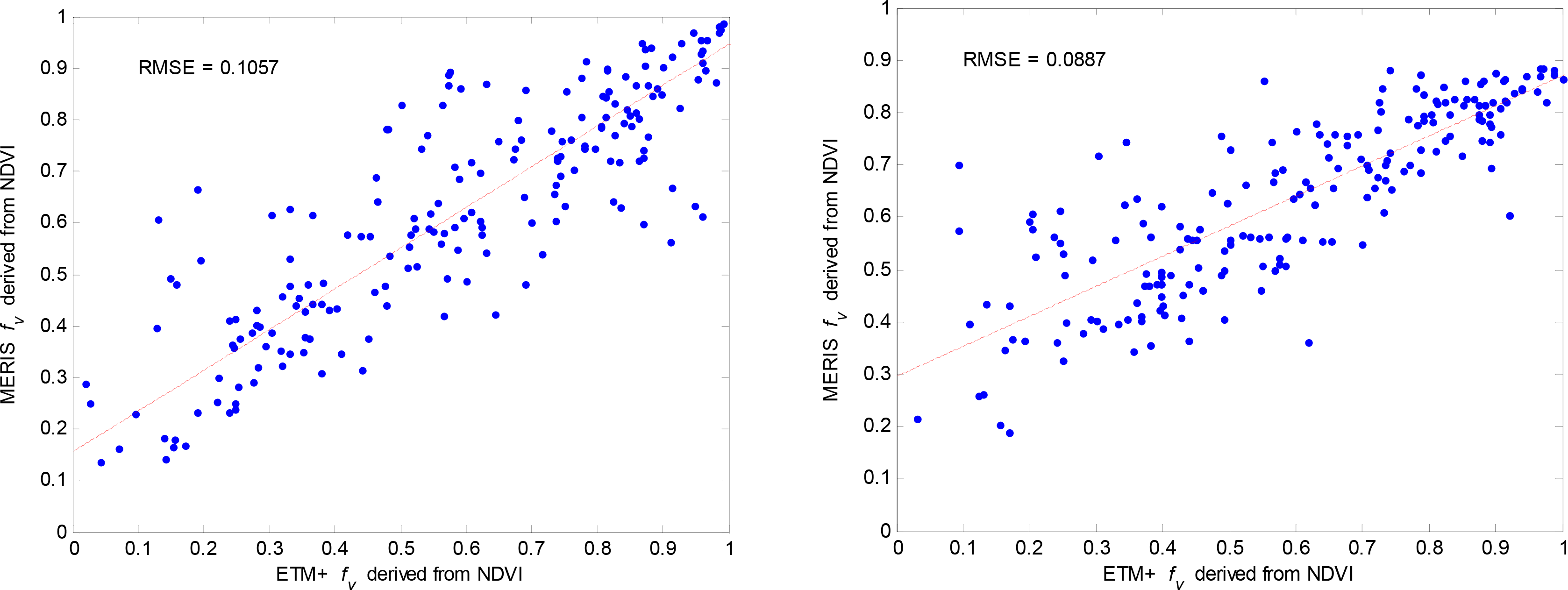
Figure 9 shows a comparison between fv derived from MERIS NDVI using the NDVI-based fv retrieval model (Equation (3)) with reference fv derived from ETM+ NDVI with the same method.
The results show an RMSE of 0.11 and 0.09 for image pair 1 and 2 respectively, indicating the level of errors incurred in estimating fv from low resolution MERIS data using NDVI-based fv retrieval model.
4.5. Spectral Unmixing
Figure 10 shows fv results of spectral unmixing of MERIS and ETM+ images. The scale indicates fv increasing from blue (open water surface) to green (fully dense vegetation cover).
As seen in the close-up of the two images, both the low and high resolution data display fv even in the sparsely populated areas. This is the advantage of spectral unmixing and similar methods which output fv, so that no vegetation information is lost however small the proportion of the pixel it covers. Of course the accuracy of the model in estimating these densities decreases with reduced resolution, but this problem is not unique to spectral unmixing.
A comparison of fv derived with spectral unmixing from MERIS imagery with those derived from the reference ETM+ data (Figure 11), shows an RMSE of 0.10 for both image pair 1 and 2, indicating the level of accuracy conceded for deriving fv at lower resolution.
The methods showed varying results when tested with two sets of samples; dense vegetation (case 1), and sparse vegetation (case 2). Sliced NDVI showed classification accuracies of 96% and 52% for case 1 and 2 respectively, indicating better performance at high vegetation densities. This heavy bias along the water-vegetation boundaries may have a significant impact on detection of sparse aquatic vegetation from coarse resolution data. Maximum likelihood classifier showed accuracies of 98% and 72% for case 1 and 2 respectively, also indicating better performance at high vegetation densities. The method of deriving fv from NDVI also showed better performance at higher vegetation densities with RMSE of 0.04 and 0.15 for case 1 and 2 respectively, because this method was designed as a dense vegetation model. Spectral unmixing showed minimal variation in the two vegetation density scales, with RMSE of 0.10 and 0.09 for case 1 and 2 respectively. These results show that detection accuracy of vegetation may vary with the density scale of vegetation cover, but with moderate effect on the results of maximum likelihood and minimal effect on the results of spectral unmixing. Spectral unmixing decomposes the pixel into various class features according to their relative abundances, and no vegetation cover information is discarded even if it constitutes a small proportion of the pixel. Spectral unmixing appears to be the most suitable method of estimating the extent of vegetation cover with coarse resolution products, but if an endmember spectral library is unavailable—due to technicalities involved in compiling it—the NDVI-based approach may be appropriate alternative, but only over dense vegetation.
Remote sensing has a huge potential of providing crucial decision support information required for the control of aquatic plants proliferation. Changes in the status of aquatic plants in inland waters sometimes occur rapidly, and thus require regular and frequent monitoring. Due to the dynamic nature of floating aquatic plants, the technique of mosaicking small pieces of high resolution remote sensing products is not feasible. For large water bodies, vegetation cover information is best derived with remote sensing products with sufficiently large swath and high acquisition frequency. Most of these products are associated with coarse spatial resolution. For each of the methods evaluated in this study, the accuracy of obtaining vegetation cover information at coarse resolution has been analysed. It is worth noting that some of the vegetation detection errors discussed may be due to geolocation errors as a result of misregistration of the image pairs, and some due to displacement of floating plants. Considering the dynamic nature of floating plants, the acquisition interval between the image pairs is crucial in assessing the accuracy of aquatic vegetation information derived at coarse resolution. The appropriate interval can be determined by considering the spatial resolution of the image pairs as well as the rate of vegetation displacement; the latter can be estimated by considering wind speed.
5. Conclusions
Timely and frequent observations of large water bodies can provide the information needed to reposition the resources at hand for interventions (e.g., mechanical removal) to mitigate the impact of aquatic vegetation. While it is desirable to use finer resolution products to accurately detect small changes in the proliferation of aquatic plants, coarse resolution products remain best suited for the management of the plants in extensive water bodies. Understanding which remote sensing techniques work best with these coarse resolution products is thus necessary. In this study we analyzed the accuracy of vegetation cover information derived from coarse resolution MERIS product in terms of delineating aquatic plants, as well as estimating its surface extent, in both cases using as reference the results obtained with Landsat-7 ETM+ acquired almost simultaneously with MERIS.
In terms of delineation of aquatic plants, we evaluated two methods: NDVI slicing and Maximum Likelihood classifier. NDVI slicing produced an average classification accuracy of 75%, but showed a lower performance of 52% over sparse vegetation, with Pareto Boundary analysis showing largest commission and omission errors in these regions. Maximum likelihood classifier showed an average classification accuracy of 80% and a lower performance of 72% over sparse vegetation. In general, maximum likelihood classifier showed better performance than NDVI slicing, and the fragmentation of vegetation cover showed lesser effect on the performance of maximum likelihood than NDVI slicing.
In terms of total area estimation, we evaluated two methods: NDVI-based vegetation fractional cover retrieval method suggested by Gutman and Ignatov [16], and linear spectral unmixing. NDVI-based approach showed an average root mean square (RMS) error of 0.097, but larger errors of 0.15 over sparse vegetation. Linear spectral unmixing showed an average RMS error of 0.096, with similar performance over dense and sparse vegetation. The two methods seem to have similar performance over dense vegetation, but while the performance of NDVI-based approach significantly drops at sparse vegetation that of spectral unmixing remains invariant with the scale of vegetation density.
In summary, among the methods evaluated in this study, we recommend maximum likelihood for the delineation of aquatic plants and spectral unmixing for estimation of its surface extent, as the methods produce more accurate results and their performances are less sensitive to the fragmentation of aquatic vegetation cover.
Acknowledgments
This research was carried out under the framework of ESA’s (European Space Agency) ALCANTARA Initiative, and was facilitated by Delft University of Technology, The Netherlands, and the University of Nairobi, Kenya. The authors acknowledge Isaiah Cheruiyot for assisting with field campaign.
Author Contributions
All authors contributed extensively to the work presented in this paper. Collins Mito, Massimo Menenti, Ben Gorte and Elijah Cheruiyot contributed to the concept design and research development. Field data was acquired by Elijah Cheruiyot, Collins Mito and Ben Gorte. Satellite data was processed by Elijah Cheruiyot and Nadia Akdim. Analysis was carried out by all authors with significant contribution from Elijah Cheruiyot and Roderik Koenders. Elijah Cheruiyot prepared the manuscript. All authors read and approved the manuscript.
Conflicts of Interest
The authors declare no conflict of interest.
References
- Albright, T.P.; Moorhouse, T.G.; McNabb, T.J. The rise and fall of water hyacinth in Lake Victoria and the Kagera River Basin, 1989–2001. J. Aquat. Plant Manag 2004, 42, 73–84. [Google Scholar]
- Silva, T.S.F.; Costa, M.P.F.; Melack, J.M.; Novo, E.M.L.M. Remote sensing of aquatic vegetation: Theory and applications. Environ. Monit. Assess 2008, 140, 131–145. [Google Scholar]
- Sawaya, K.E.; Olmanson, L.G.; Heinert, N.J.; Brezonik, P.L.; Bauer, M.E. Extending satellite remote sensing to local scales: Land and water resource monitoring using high-resolution imagery. Remote Sens. Environ 2003, 88, 144–156. [Google Scholar]
- Govender, M.; Chetty, K.; Bulcock, H. A review of hyperspectral remote sensing and its application in vegetation and water resource studies. Water SA 2007, 33, 145–152. [Google Scholar]
- Latifovic, R.; Olthof, I. Accuracy assessment using sub-pixel fractional error matrices of global land cover products derived from satellite data. Remote Sens. Environ 2004, 90, 153–165. [Google Scholar]
- Congalton, R.G. A review of assessing the accuracy of classifications of remotely sensed data. Remote Sens. Environ 1991, 37, 35–46. [Google Scholar]
- Kitada, K.; Fukuyama, K. Land-use and land-cover mapping using a gradable classification method. Remote Sens 2012, 4, 1544–1558. [Google Scholar]
- Kindu, M.; Schneider, T.; Teketay, D.; Knoke, T. Land use/land cover change analysis using object-based classification approach in munessa-shashemene landscape of the ethiopian highlands. Remote Sens 2013, 5, 2411–2435. [Google Scholar]
- De Asis, A.M.; Omasa, K.; Oki, K.; Shimizu, Y. Accuracy and applicability of linear spectral unmixing in delineating potential erosion areas in tropical watersheds. Int. J. Remote Sens 2008, 29, 4151–4171. [Google Scholar]
- Cavalli, R.M.; Laneve, G.; Fusilli, L.; Pignatti, S.; Santini, F. Remote sensing water observation for supporting Lake Victoria weed management. J. Environ. Manag 2009, 90, 2199–2211. [Google Scholar]
- Viña, A.; Gitelson, A.A.; Nguy-Robertson, L.A.; Peng, Y. Comparison of different vegetation indices for the remote assessment of green leaf area index of crops. Remote Sens. Environ 2011, 115, 3468–3478. [Google Scholar]
- Ouma, G.; Omeny, P.A.; Kabubi, J. Remote sensing application on eutrophication monitoring in Kavirondo Gulf of Lake Victoria Kenya. J. Afr. Meteorol. Soc 2003, 6, 11–18. [Google Scholar]
- Kiage, L.M.; Obuoyo, J. The potential link between el nino and water hyacinth blooms in winam gulf of Lake Victoria, East Africa: Evidence from satellite imagery. Water Resour. Manag 2011, 25, 3931–3945. [Google Scholar]
- Omute, P.; Corner, R.; Awange, J.L. The use of NDVI and its derivatives for monitoring Lake Victoria’s water level and drought conditions. Water Resour. Manag 2012, 26, 1591–1613. [Google Scholar]
- Fusilli, L.; Collins, M.O.; Laneve, G.; Palombo, A.; Pignatti, S.; Santini, F. Assessment of the abnormal growth of floating macrophytes in Winam Gulf (Kenya) by using MODIS imagery time series. Int. J. Appl. Earth Obs. Geoinf 2013, 20, 33–41. [Google Scholar]
- Gutman, G.; Ignatov, A. The derivation of the green vegetation fraction from NOAA/AVHRR data for use in numerical weather prediction models. Int. J. Remote Sens 1998, 19, 1533–1543. [Google Scholar]
- Aloo, P.; Ojwang, W.; Omondi, R.; Njiru, J.M.; Oyugi, D. A review of the impacts of invasive aquatic weeds on the bio-diversity of some tropical water bodies with special reference to Lake Victoria (Kenya). Biodivers. J 2013, 4, 471–482. [Google Scholar]
- Plummer, M.L. Impact of invasive water hyacinth (eichhornia crassipes) on snail hosts of schistosomiasis in Lake Victoria, East Africa. EcoHealth 2005, 2, 81–86. [Google Scholar]
- Mailu, A.M.; Ochiel, G.R.S.; Gitonga, W.; Njoka, S.W. Water hyacinth: An environmental disaster in the Winam Gulf of Lake Victoria and its control. Proceedings of the First IOBC Global Working Group Meeting for the Biological and Integrated Control of Water Hyacinth, Harare, Zimbabwe, 16–19 November 1998; Hill, M.P., Julien, M.H., Center, T.D., Eds.; pp. 101–105.
- Kay, S.; Hedley, J.D.; Lavender, S. Sun glint correction of high and low spatial resolution images of aquatic scenes: A review of methods for visible and near-infrared wavelengths. Remote Sens 2009, 1, 697–730. [Google Scholar]
- Dekker, A.G.; Byrne, G.T.; Brando, V.E.; Anstee, J.M. Hyperspectral Mapping of Intertidal Rock Platform Vegetation as a Tool for Adaptive Management; CSIRO Land and Water: Acton, Australia, 2003. [Google Scholar]
- Rahman, H.; Dedieu, G. SMAC: A simplified method for the atmospheric correction of satellite measurements in the solar spectrum. Int. J. Remote Sens 1994, 15, 123–143. [Google Scholar]
- Jackson, R.D.; Huete, A.R. Interpreting vegetation indices. Prev. Vet. Med 1991, 11, 185–200. [Google Scholar]
- Rouse, J.W.; Haas, R.H.; Schell, J.A. Monitoring the Vernal Advancement and Retrogradation (Greenwave Effect) of Natural Vegetation; Texas A&M University: College Station, TX, USA, 1974. [Google Scholar]
- Haboudane, D. Hyperspectral vegetation indices and novel algorithms for predicting green LAI of crop canopies: Modeling and validation in the context of precision agriculture. Remote Sens. Environ 2004, 90, 337–352. [Google Scholar]
- Elmore, A.J.; Mustard, J.F.; Manning, S.J.; Lobell, D.B. Quantifying vegetation change in semiarid environments: Precision and accuracy of spectral mixture analysis and the normalized difference vegetation index. Remote Sens. Environ 2000, 73, 87–102. [Google Scholar]
- Lunetta, R.S.; Knight, J.F.; Ediriwickrema, J.; Lyon, J.G.; Worthy, L.D. Land-cover change detection using multi-temporal MODIS NDVI data. Remote Sens. Environ 2006, 105, 142–154. [Google Scholar]
- Zhang, J.; Liu, Z.; Sun, X. Changing landscape in the three gorges reservoir area of Yangtze River from 1977 to 2005: Land use/land cover, vegetation cover changes estimated using multi-source satellite data. Int. J. Appl. Earth Obs. Geoinf 2009, 11, 403–412. [Google Scholar]
- Ma, R.; Duan, H.; Gu, X.; Zhang, S. Detecting aquatic vegetation changes in Taihu Lake, China using multi-temporal Satellite Imagery. Sensors 2008, 8, 3988–4005. [Google Scholar]
- Jiang, Z.; Huete, A.R.; Chen, J.; Chen, Y.; Li, J.; Yan, G.; Zhang, X. Analysis of NDVI and scaled difference vegetation index retrievals of vegetation fraction. Remote Sens. Environ 2006, 101, 366–378. [Google Scholar]
- Johnson, B.; Tateishi, R.; Kobayashi, T. Remote Sensing of fractional green vegetation cover using spatially-interpolated endmembers. Remote Sens 2012, 4, 2619–2634. [Google Scholar]
- Adams, J.B.; Smith, M.O.; Johnson, P.E. Spectral mixture modeling: A new analysis of rock and soil types at the Viking Lander 1 site. J. Geophys. Res. Solid Earth 1986, 91, 8098–8112. [Google Scholar]
- Smith, M.O.; Ustin, S.L.; Adams, J.B.; Gillespie, A.R. Vegetation in deserts: I. A regional measure of abundance from multispectral images. Remote Sens. Environ 1990, 31, 1–26. [Google Scholar]
- Adams, J.B.; Sabol, D.E.; Kapos, V.; Filho, R.A.; Roberts, D.A.; Smith, M.O.; Gillespie, A.R. Classification of multispectral images based on fractions of endmembers: Application to land-cover change in the Brazilian Amazon. Remote Sens. Environ 1995, 52, 137–154. [Google Scholar]
- Small, C. Estimation of urban vegetation abundance by spectral mixture analysis. Int. J. Remote Sens 2001, 22, 1305–1334. [Google Scholar]
- Liu, W.; Wu, E.Y. Comparison of non-linear mixture models: Sub-pixel classification. Remote Sens. Environ 2005, 94, 145–154. [Google Scholar]
- Theseira, M.A.; Thomas, G.; Sannier, C.A.D. An evaluation of spectral mixture modelling applied to a semi-arid environment. Int. J. Remote Sens 2002, 23, 687–700. [Google Scholar]
- Hartigan, A. Clustering Algorithms; Wiley: Hoboken, NJ, USA, 1975. [Google Scholar]
- Hartigan, J.A.; Wong, M.A. Algorithm AS 136: A k-means clustering algorithm. Appl. Stat 1979, 28, 100–108. [Google Scholar]
- Boschetti, L.; Flasse, S.P.; Brivio, P.A. Analysis of the conflict between omission and commission in low spatial resolution dichotomic thematic products: The Pareto Boundary. Remote Sens. Environ 2004, 91, 280–292. [Google Scholar]


| Image Pair | Sensor | Acquisition Time | Spatial Resolution | Spectral Resolution (Visible and NIR) | Sensor Viewing Angles |
|---|---|---|---|---|---|
| Pair 1 | MERIS | 15 December 2010 07:49 | 300 m | 15 bands | 7°–11° |
| ETM+ | 15 December 2010 07:48 | 30 m | 5 bands | 0°–5° | |
| Pair 2 | MERIS | 27 July 2011 07:41 | 300 m | 15 bands | 6°–10° |
| ETM+ | 27 July 2011 07:48 | 30 m | 5 bands | 0°–5° | |
| MERIS | ETM+ | Comparison method | ||
|---|---|---|---|---|
| Method | Retrievals | Method | Retrievals | |
| -- | -- | Delineation | -- | -- |
| Sliced NDVI | 3 classes | Sliced NDVI | 3 classes | Error matrix |
| Maximum Likelihood | 2 classes | Maximum Likelihood | 2 classes | Error matrix |
| -- | -- | Total area | -- | -- |
| NDVI | fv | NDVI | fv | RMSE, Linear regression |
| Spectral unmixing | fv | Spectral unmixing | fv | RMSE, Linear regression |
| Reference (ETM+) | Commission Error | Reference (ETM+) | Commission Error | ||||||||||
|---|---|---|---|---|---|---|---|---|---|---|---|---|---|
| FV | SV | OW | Row Total | FV | SV | OW | Row Total | ||||||
| Classified (MERIS) | FV | 85 | 12 | 1 | 98 | 13% | Classified (MERIS) | FV | 89 | 9 | 3 | 101 | 12% |
| SV | 16 | 17 | 6 | 39 | 56% | SV | 10 | 17 | 16 | 43 | 60% | ||
| OW | 3 | 9 | 51 | 63 | 19% | OW | 1 | 15 | 40 | 56 | 29% | ||
| Column Total | 104 | 38 | 58 | 200 | Column Total | 100 | 41 | 59 | 200 | ||||
| Omission Error | 18% | 55% | 12% | Omission Error | 11% | 59% | 32% | ||||||
| Reference (ETM+) | Commission Error | Reference (ETM+) | Commission Error | ||||||||
|---|---|---|---|---|---|---|---|---|---|---|---|
| FV | OW | Row Total | FV | OW | Row Total | ||||||
| Classified (MERIS) | FV | 99 | 34 | 133 | 26% | Classified (MERIS) | FV | 96 | 38 | 134 | 28% |
| OW | 3 | 64 | 67 | 4% | OW | 5 | 61 | 66 | 8% | ||
| Column Total | 102 | 98 | 200 | Column Total | 101 | 99 | 200 | ||||
| Omission Error | 3% | 35% | Omission Error | 5% | 38% | ||||||
© 2014 by the authors; licensee MDPI, Basel, Switzerland This article is an open access article distributed under the terms and conditions of the Creative Commons Attribution license (http://creativecommons.org/licenses/by/3.0/).
Share and Cite
Cheruiyot, E.K.; Mito, C.; Menenti, M.; Gorte, B.; Koenders, R.; Akdim, N. Evaluating MERIS-Based Aquatic Vegetation Mapping in Lake Victoria. Remote Sens. 2014, 6, 7762-7782. https://0-doi-org.brum.beds.ac.uk/10.3390/rs6087762
Cheruiyot EK, Mito C, Menenti M, Gorte B, Koenders R, Akdim N. Evaluating MERIS-Based Aquatic Vegetation Mapping in Lake Victoria. Remote Sensing. 2014; 6(8):7762-7782. https://0-doi-org.brum.beds.ac.uk/10.3390/rs6087762
Chicago/Turabian StyleCheruiyot, Elijah K., Collins Mito, Massimo Menenti, Ben Gorte, Roderik Koenders, and Nadia Akdim. 2014. "Evaluating MERIS-Based Aquatic Vegetation Mapping in Lake Victoria" Remote Sensing 6, no. 8: 7762-7782. https://0-doi-org.brum.beds.ac.uk/10.3390/rs6087762