Wheat Yield Forecasting for Punjab Province from Vegetation Index Time Series and Historic Crop Statistics

 ,
,
Abstract
: Policy makers, government planners and agricultural market participants in Pakistan require accurate and timely information about wheat yield and production. Punjab Province is by far the most important wheat producing region in the country. The manual collection of field data and data processing for crop forecasting by the provincial government requires significant amounts of time before official reports can be released. Several studies have shown that wheat yield can be effectively forecast using satellite remote sensing data. In this study, we developed a methodology for estimating wheat yield and area for Punjab Province from freely available Landsat and MODIS satellite imagery approximately six weeks before harvest. Wheat yield was derived by regressing reported yield values against time series of four different peak-season MODIS-derived vegetation indices. We also tested deriving wheat area from the same MODIS time series using a regression-tree approach. Among the four evaluated indices, WDRVI provided more consistent and accurate yield forecasts compared to NDVI, EVI2 and saturation-adjusted normalized difference vegetation index (SANDVI). The lowest RMSE values at the district level for forecast versus reported yield were found when using six or more years of training data. Forecast yield for the 2007/2008 to 2012/2013 growing seasons were within 0.2% and 11.5% of final reported values. Absolute deviations of wheat area and production forecasts from reported values were slightly greater compared to using the previous year’s or the three- or six-year moving average values, implying that 250-m MODIS data does not provide sufficient spatial resolution for providing improved wheat area and production forecasts.1. Introduction
Pakistan is anticipating massive population growth over the coming decades. Population size is projected to increase from 185 million in 2014 to 271 million by 2050, which is nearly as high as the current U.S. population, while only occupying an area equivalent to eight percent of the U.S. land area [1]. Food production has not increased at the same rate as human population, resulting in concerns for food security. More severe droughts and floods due to global climate change are expected to negatively impact food availability [2]. Accurate and timely information provided through large-scale monitoring of crop production and yield forecasting is an essential tool to help address these concerns.
The most important food crop in Pakistan is wheat, which is cultivated during the Rabi season (winter season) on the majority of agricultural land in the Punjab province [3]. Wheat contributes 12.5% to the value added to GDP in agriculture and accounts for 2.6% of total GDP [4]. Accurate wheat production forecasts allow government planners, policy experts and decision makers to better determine whether and how much grain to import or export, while maintaining adequate reserves for national food security and to set support prices at appropriate levels. The effect of inaccurate forecasts was exemplified in 2005 when a large surplus of wheat was expected in Pakistan, allowing private traders to purchase wheat significantly below the support price and triggering the government to sell wheat grain on the international markets, while the final production was much lower than expected, caused by damage from rains and strong winds [5,6].
The conventional system employed by the provincial government for collecting agricultural statistical data relies on labor- and time-intensive field data collection in a small percentage of villages. The sample villages are selected at random, stratified by village size and do not represent all agricultural areas equally within a cropping season, and field data are not collected from inaccessible areas. The list frame system is based on an extensive system of crop reporters in the field and is effective in the provision of data for agricultural management. However, the data are acquired through manual surveys and enumeration techniques, and data compilation and analysis are only completed several months after harvest. As a result, the use of these data for timely decision making and adequate planning for wheat shortages or surplus is limited [7].
The use of satellite remote sensing and geographic information system (GIS) technologies for agricultural monitoring and estimating crop yield and production has a long history from the first civilian applications of air- and space-borne remote sensing imagery, which were focused on agricultural monitoring [8], to the Large Area Crop Inventory Experiment (LACIE) [9] and Agricultural and Resources Inventory Surveys Through Aerospace Remote Sensing (AgRISTARS) [10] programs. The Monitoring Agricultural Resources Unit (MARS) Crop Yield Forecasting System (MCYFS) currently provides seasonal yield forecasts for key European crops, through a system combining remote sensing, meteorological and agro-meteorological data and biophysical models [11]. The Global Agricultural Monitoring Project (GLAM), a joint initiative of NASA, the US Department of Agriculture (USDA) and the University of Maryland, has built an operational system for global satellite-based crop condition monitoring as part of the Decision Support System (DSS) of the USDA Foreign Agricultural Service (FAS) [12]. Bastiaanssen and Ali [13] used AVHRR satellite data and a deterministic model to forecast crop yield across the Indus Basin in Pakistan. Most recently, the national space agency, Pakistan Space and Upper Atmosphere Research Commission (SUPARCO), together with the Food and Agricultural Organization of the United Nations (UN-FAO) developed an area frame system utilizing SPOT satellite data for obtaining agricultural statistics on crop yield and production of wheat and other crops and is publishing a monthly crop bulletin [14].
The first objective of this study is to develop and test the use of remote sensing technology for early season yield forecasting in Punjab Province, Pakistan, with the goal of providing a tool complementing the existing system based on field surveys. The aim is to provide first approximations of wheat yield before the final results using the conventional system become available to help improve timely decision-making. The second objective of the study is to improve existing methods based on regressing time series of NDVI against reported yield by testing different vegetation indices for Punjab Province under the local conditions, which are characterized by smaller and more diverse fields than many other wheat-producing countries for which these kind of relationships have been typically tested.
In this study, we developed a methodology for forecasting wheat yield for the Punjab Province using time series of satellite imagery and historic crop statistics. We also tested the production of wheat area maps for production forecasting. Already existing global-scale crop maps, such as [15], typically suffer from varying spectral phenologies at the global scale and can be improved upon when applied locally. Wheat area maps were generated from a time series of Moderate Resolution Imaging Spectroradiometer (MODIS) eight-day composite satellite imagery converted to seasonal metrics using a bagged decision tree approach [16]. This method and the selection of metrics is based on previous work by [17–19] and others derived from AVHRR, MODIS and Landsat time series and a decision tree methodology for mapping tree cover. The temporal signature inherent in the MODIS time series can be used to distinguish major crop types [20,21]. MODIS time series transformed into seasonal metrics capture salient points in the vegetation phenological cycle and represent generic signatures, which allow one to determine crop types over large areas [22]. Chang et al. [23] used 279 annual metrics calculated from MODIS 32-day composites to estimate areas of corn and soybean in the U.S. with high accuracy.
2. Materials
In this study, we developed regression-based models for estimating wheat area, yield and production prior to harvest for the Punjab Province of Pakistan from satellite remote sensing data and historic, reported crop statistics. The model developed by [24] for Kansas was adapted and re-written in the Python programming language, and model parameters were calibrated to local conditions. Three principal data sources were used in this study: (1) Landsat TM and ETM satellite imagery; (2) MODIS 8-day composites; and (3) historic, reported crop statistics for wheat yield, area and production. The Landsat data were used to train a decision tree classifier for estimating crop area from MODIS-derived seasonal metrics. The MODIS composites were also used to forecast yield by regressing crop statistics against MODIS-derived vegetation indices.
2.1. Study Site
Agriculture is of central importance to Pakistan. The agricultural sector overall contributes approximately 20% to GDP each year and fetches 80% of the country’s total export earnings. The agriculture sector plays a vital role for food security, poverty reduction and overall economic growth. The majority of the rural population depends on agriculture for their livelihoods. The study area of this research project is Punjab, the central province and main wheat producing region of Pakistan. Punjab Province covers more than 70% of the total cropped area nation-wide and, over the last year, accounted, on average, for 74% of national wheat production [4].
Punjab Province is a fertile region covered by thick layers of alluvium deposited by five major rivers flowing down from the rapidly eroding Himalayan Mountains south into the Indus River Delta and the Arabian Sea. The extensive alluvial plain gently slopes from an altitude of approximately 500 m.a.s.l. to 100 m.a.s.l. [25].
Pakistan has two main cropping seasons, the summer season (Kharif, meaning autumn) from mid April to mid October, during which time the annual monsoon rains occur, and the winter season (Rabi, meaning spring) from mid-October to mid-April. The main crops in the Kharif season are rice, cotton, sugarcane and maize. The principal crop in the Rabi season is wheat. Sowing of wheat takes place between the end of October and mid-December, and harvesting occurs during the months of April and early May. The climate is dry with an annual precipitation gradient from 100 mm in the south to 600 mm in the northwest, reaching up to 1000 mm along the northeastern boundary. Nearly three quarters of annual precipitation fall in the monsoon months June to September before the start of the Rabi season [26]. Cumulative evapotranspiration of wheat during the Rabi season typically ranges from 200 mm to 500 mm and can reach up to 800 mm under heavy irrigation [27]. As a consequence, precipitation in Punjab is insufficient in most areas to support wheat production, and the vast majority of wheat fields are irrigated. Only the Potohar plateau in the north supports large areas of rainfed agriculture.
Pakistan has the largest contiguous irrigation system in the world. The irrigation system was massively expanded after separation from India through the 1960s and 1970s. Today, the irrigation system faces numerous challenges. Per capita availability of water has been decreasing steadily. Water productivity measured as crop yield per cubic meter water is comparatively low. Loss of water reservoir capacity from sedimentation is increasing, and water supply through the Indus River system is expected to decrease in the future, due to climate change [2]. Any change in the supply of irrigation water will directly impact agricultural production, emphasizing the need of crop condition monitoring during the growing season and timely and accurate crop yield and production forecasts.
2.2. Landsat Data
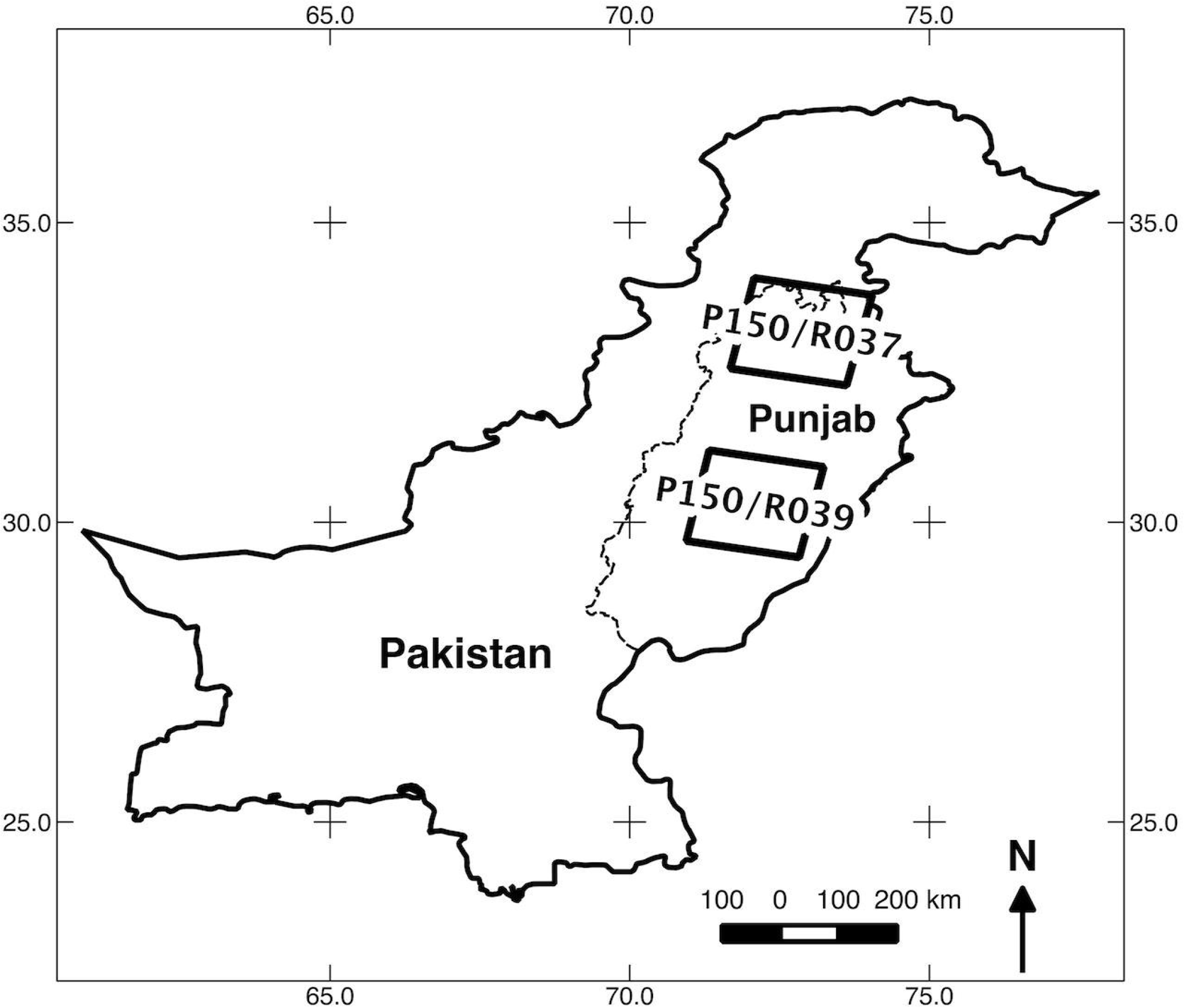
We used satellite imagery from both the Landsat 7 ETM and Landsat 5 TM satellite instruments to derive training data for driving the wheat classification of the MODIS time series. For each Rabi season from 2001/2002 to 2009/2010, we selected three Landsat images for each of two locations in Punjab Province, one in central Punjab with low rainfall dominated by irrigated agriculture and one in northern Punjab with higher rainfall and a higher proportion of rainfed agriculture (Figure 1). The combined area of both Landsat scenes comprise 28.1% of the area of Punjab, which was considered a sufficiently large subset to serve as training.
The first of the three seasonal images was from the early growing season after crop emergence (January), the second from the height of the growing season (mid-February to mid-March) and the third after harvest (mid-April to mid-May). The total number of images used for training was 54 (Table 1). Bands 1 (blue) and 2 (green) were excluded because of their sensitivity to atmospheric disturbances. Bands 3 (red), 4 (near-infrared), 5 (mid-infrared), 6 (thermal, resampled to 30 m) and 7 (shortwave-infrared) were used for the analysis.
2.3. MODIS Data
In this study, we used MODIS data for two purposes, for yield forecasting and for mapping the presence of wheat. For yield forecasting, we used a time series of 8-day, clear-sky MODIS surface reflectance composites at 250-m resolution (MODIS science product MOD09Q1) from 31 October 2001 to 24 May 2013. The composited imagery represents the best available observation per pixel for each 8-day period. Low-quality pixels with MODIS quality assurance (QA) bits indicating clouds, cloud adjacency, cloud shadows, water, high level of aerosols, cirrus clouds, fire and snow/ice were excluded from the analysis (Table 2).
The 8-day composites of the three MODIS tiles overlapping the study area (MODIS tile numbers h23/v05, h24/v05 and h24/v06) were mosaicked together, reprojected to the sinusoidal projection with a sphere radius 6,371,007.181 m and central meridian 75 degrees east, subset to the area of Punjab Province and converted to the NDVI, saturation-adjusted normalized difference vegetation index (SANDVI), EVI2 and WDRVI indices. All indices were scaled from 0 to 250 and stored in 8-bit format.
For the per pixel characterization of wheat presence in the Punjab province, we used a multi-year time series of MODIS 8-day composites from the Rabi season 2001/2002 to 2012/2013 between the growing season dates 3 December and 26 February. Time series of three of the seven MODIS spectral land bands, one thermal band and two derived spectral indices were converted to seasonal metrics in order to reduce the effects of residual cloud cover and to enhance the development of the generic model of wheat presence per 250-m MODIS pixel across multiple years. The MODIS inputs consisted of Band 1 (620–670 nm, red) and Band 2 (841–876 nm, near-infrared) at 250-m spatial resolution, Band 7 (2105–2155 nm, short-wave infrared) at 500-m resolution and Band 31 (10,780–11,280 nm, thermal) at 1-km resolution. The thermal and short-wave infrared data were resampled to 250-m resolution. The normalized difference water index (NDWI) was calculated as NDWI = (NIR − SWIR)/(NIR + SWIR), where NIR is the near-infrared band and SWIR the short-wave infrared band.
2.4. Official Crop Statistics
The Crop Reporting Service (CRS) of the Government of Punjab produces official agricultural statistics for wheat and other crops for all 36 Punjab districts. CRS Punjab was founded in 1978 and employs more than one thousand crop reporters collecting field data in 1240 villages (5% of the total number of villages) throughout the province. The list of villages was compiled by CRS through random selection within three strata based on village size. The village list is updated every five years. Statistical experts at CRS interpret and aggregate the collected data to the district and provincial levels and calculate estimates for crop yield, area and production. The field personnel also reports on crop conditions fortnightly and on weather conditions weekly [28].
The CRS produces three official estimates for the wheat crop. The first crop inspection is carried out in January after completion of sowing. This field survey is the basis for the first estimate of wheat cultivated area, released on 1 February of each year. The second inspection in late February and early March surveys production inputs and crop condition and generates a list of all wheat growing fields in each sample village, the so-called wheat crop frame. From these data, CRS statistical experts derive the expected crop production and release the forecast on 1 April, before the beginning of the harvest period. The third inspection takes place during harvest when the crop reporters measure yield in experimental plots of a size 20 ft × 15 ft (28 square meters). Two of the measurement plots are placed at random within each of three randomly selected wheat fields per village. The final wheat area estimate is derived from a complete census. The complete census is an estimate of area sown under all crops and based on the enumeration of all districts carried out by government land tenure officials of the Pakistan Revenue Department for tax purposes. CRS calculates the final production estimates by multiplying measured yield values with the final area values. CRS reports the final data to the Government of Pakistan by 1 August of each year [28].
3. Methods
The methodology has two main components. In the first component, we calculate spatial data layers of percent wheat per 250-m MODIS pixel. The wheat coverage layers are used for identifying pixels with high wheat percentage as input for the yield forecasting model and for testing the estimation of wheat crop area. In the second component, we develop wheat yield regression models and apply them to the forecast years.
3.1. Landsat Classification
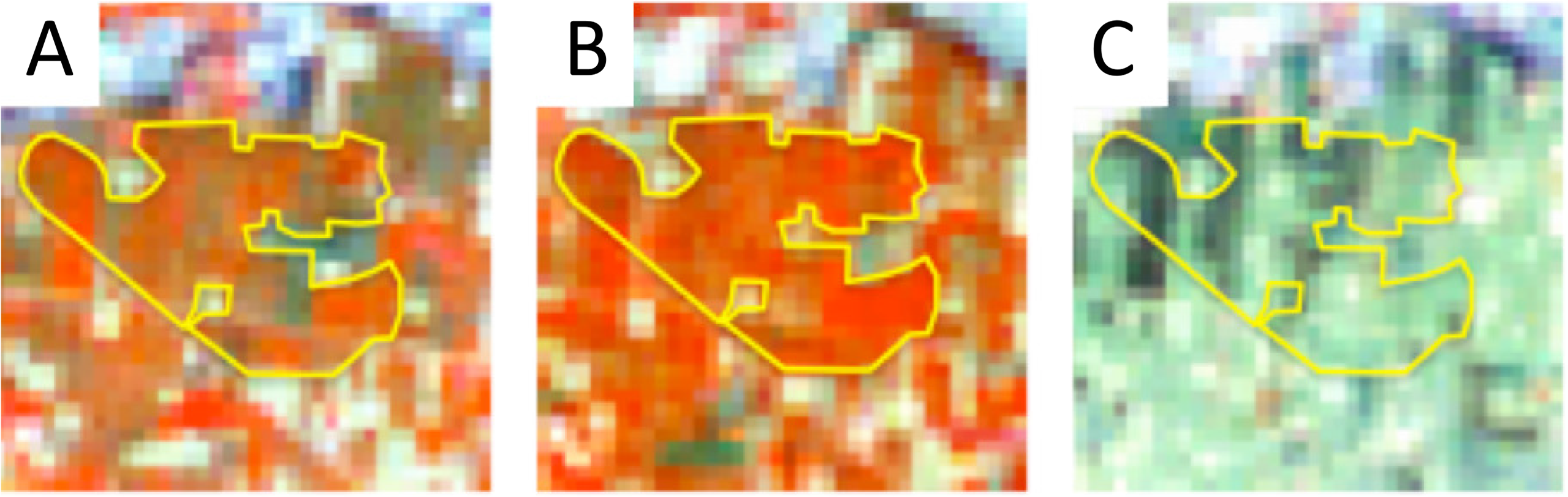
Landsat 7 ETM imagery at processing level 1T was acquired from the U.S. Geological Survey (USGS). The imagery consists of radiometrically and geometrically corrected at-aperture spectral radiance, scaled to 8-bit digital numbers. For each Rabi season, we stacked Bands 3 to 7 of the three selected Landsat scenes per location into a single data file and classified it for wheat/non-wheat on a pixel-by-pixel basis. Clouds and stripes of missing data pixels resulting from the malfunctioning Landsat scan-line corrector (SLC) were masked out. This was repeated for the two path/row locations. Training data for the classification were selected by visual interpretation of the Landsat time series, based on the phenology of wheat, which was familiar to the analyst from previous work in other wheat-growing areas in Kansas and Ukraine [24]. The vast majority of winter wheat in Pakistan is sown in November and December and harvested in April. This is clearly visible in time sequences of Landsat scenes. When displayed in the band combination, 4-5-3, wheat fields appear light red in the early growing season (January), bright red at the height of the growing season (mid-February to mid-March) and blue/purple after maturity or dark green after harvest (mid-April to mid-May), as displayed in Figure 2.
At each path/row, we selected approximately 8 to 20 training polygons of wheat fields and a similar number of non-wheat polygons, preferably directly adjacent to each other. This helps in training the algorithm to detect boundaries between the two land cover types. Additional non-wheat training pixels were selected throughout the image from visually discernible non-wheat areas.
For classifying the Landsat data, we used a bagged decision tree approach [16]. The reflectance values for each training pixel of all 15 stacked Landsat bands served as the input to the decision tree algorithm. The algorithm recursively splits the training data into subsets, or nodes, using a reflectance band threshold, so that each new node has maximum homogeneity measured as the minimum overall residual sum of squares or deviance. This way, the data are split at each node into two subsets, and a binary decision tree is incrementally developed. For the bagging procedure, a total of seven decision trees was calculated, each using a 20% subset of the complete set of training data, selected at random with replacement. All seven trees were applied to the entire image area. Membership of the pixels to each of the two classes, wheat or non-wheat, was determined by selecting the majority of the seven resulting values (voting). The analyst inspected the result visually and, if not satisfactory, selected additional training pixels in incorrectly classified areas. Using the expanded set of training data, the bagged decision tree classification process was repeated and again evaluated by visual interpretation of the results. This process was repeated again until the results were satisfactory to the trained eye of the analyst. The final result was reprojected to the sinusoidal projection of the MODIS imagery composites and aggregated to a pixel size of 250-m resolution, resulting in a percent wheat value for each MODIS pixel.
3.2. MODIS Classification
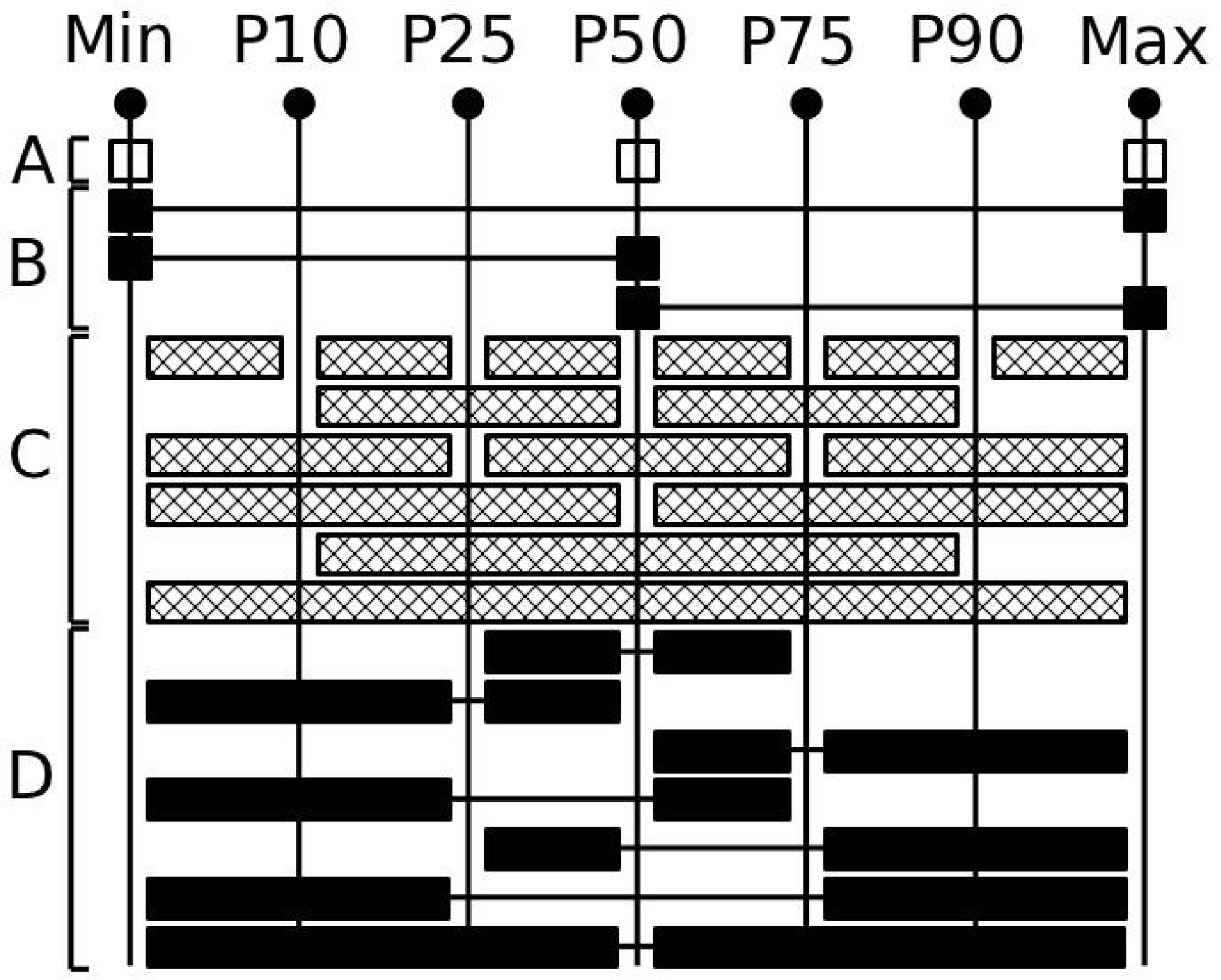
Percent wheat data layers were generated for all 12 Rabi seasons 2001/2002 to 2012/2013 using MODIS data as inputs/explanatory variables and training data from the nine Rabi seasons between 2001/2002 and 2009/2010. The classification inputs were derived from time series of three of the seven MODIS 8-day composites land bands, a thermal band and two derived spectral indices, NDVI and NDWI. These spectral bands and their respective indices were converted to seasonal metrics representing a single dataset of phenological characteristics for a given pixel for each Rabi season. This was facilitated by first sorting, by pixel, all seasonal composites of each input band and each index and employing the sorted data to produce a set of 28 metrics. The metrics for each of the input bands were calculated based on the 0th (minimum), 10th, 25th, 50th (median), 75th, 90th and 100th (maximum) percentiles, as illustrated in Figure 3.
The metrics consist of the minimum, median and maximum (3 values), the amplitudes between minimum, median and maximum (3 values), the mean values of ranges of percentiles (15 values) and the amplitudes between percentile means (7 values). This set of the same 28 metrics was created for each of the 3 spectral bands, the thermal band, the NDVI and NDWI indices, as well as for the 15 ranked combinations between them, as shown in Table 3, resulting in a total of 28 × 21 = 588 growing season metrics.
For example, when ranking the red band by the NDVI band, the corresponding red band values were selected at the point in time at which the NDVI band values were at the 0th, 10th, 25th, etc., percentile. A generalized bagged decision tree model for estimating percent wheat per pixel for all years was calculated using the 588 seasonal metrics of the Rabi seasons 2001/2002 to 2009/2010 combined as independent variables. The Landsat-derived training data were used as the dependent variable to calculate 7 bagged decision trees; each tree using 20% of the training data, selected at random with replacement. The bagging methodology was introduced by [16] and reduces classification error resulting from noise, bias and variance of the training data sample by calculating an ensemble of decision trees, each derived from a different random subset of the entire training data set and averaging the classification results. The resulting set of 7 decision trees was then applied to each forecast year, and percent wheat estimates were calculated for each 250-m pixel. The 7 output percent values were then ranked and the median result of the 7 used as the final result ranging from 0% to 100% wheat presence.
3.3. Vegetation Indices
Estimating wheat yield was tested by exploiting the relationship with peak-season normalized difference vegetation index (NDVI), the saturation-adjusted normalized difference vegetation index (SANDVI), the two-band enhanced vegetation index (EVI2) and the wide dynamic range vegetation index (WDRVI) and comparing the performance of each index.
Previous studies have found strong correlations between wheat yield and NDVI. Tucker et al. [29] explained 79% of the variation in total wheat dry-matter accumulation by integrating NDVI over the growing season. Labus et al. [30] calculated NDVI from an AVHRR time series for the U.S. state of Montana and found strong correlations between wheat yield and integrated NDVI, as well as late-season NDVI parameters. Mkhabela et al. [31] forecasted the yield of major crops in the Canadian Prairies, including spring wheat, using 10-day MODIS NDVI composites. Dempewolf et al. [32] achieved good agreement between wheat yield derived from MODIS-derived NDVI and reported yield for the 2011/2012 growing season for Punjab Province, Pakistan. The forecast of yield for the majority of cases was within 10% of final reported values. Ren et al. [33] used 10-day MODIS NDVI composites to forecast the yield of winter wheat for a sub-region of Shandong Province in China, and the results were within 5% of official statistics. Meroni et al. [34] examined the performance of spectral parameters derived from SPOT-VEGETATION data for wheat yield forecasting in Tunisia and, for NDVI, achieved an r-squared value of 0.75 between modeled and observed yield. Becker-Reshef et al. [24] used a daily surface reflectance MODIS dataset to develop an empirical, regression-based model for forecasting wheat yield for the U.S. state of Kansas. When using the same model for forecasting wheat yield in Ukraine, the results showed high accuracy. The methodology developed for this study builds on the same approach. An overview of further studies investigating the link between the yield of a variety of crops and NDVI derived from a number of different satellite sensors is provided by [35]. NDVI was calculated as NDVI = (NIR − R)/(NIR + R), where R is the red band and NIR the near-infrared band [36]. NDVI fractions were capped to the range −0.25 to 1.0.
SANDVI was designed by [37] (called NDVIsat−adjust) to adjust high, saturated NDVI values by replacing them with a linear function of the near-infrared-to-red band ratio. The authors compared the 10-year SANDVI growing-season average in the Greater Platte River Basin, USA, with ground observations of corn yield of the same time period and found improved agreement between the two data sets compared to using non-adjusted NDVI (r = 0.78 versus r = 0.67, 113 samples).
SANDVI is equal to NDVI for NDVI values up to 0.78. Beyond that, SANDVI is calculated as a linear function of the ratio vegetation index (RVI) (Equation (1)). The function was derived by regressing RVI against NDVI in the range 0.7 to 0.8, for which both indices have a very similar linear distribution [37]. SANDVI values were capped to the range −0.25 to 1.0.
The enhanced vegetation index (EVI) was designed as an improvement over NDVI under high green biomass conditions where NDVI saturates. It includes a soil adjustment factor, as well as an atmosphere resistance term, based on blue band reflectance [38]. EVI has been found to be more responsive to variations in leaf area index (LAI), canopy type and architecture [39], but is limited to sensor systems incorporating a blue band, in addition to the red and near-infrared bands. This makes it difficult to take full advantage of the high 250-m spatial resolution of the MODIS red and near-infrared bands. Jiang et al. [40] developed a 2-band EVI (EVI2) without the blue band, using the red and near-infrared bands only and found that EVI2 corresponds well to EVI when atmospheric effects are insignificant and data quality is high.
EVI2 was calculated as shown in Equation (2). EVI2 values were capped to the range −0.25 to 1.25.
WDRVI was introduced by [41] and shows increased sensitivity to crop physiological and phenological characteristics for leaf area index (LAI) values over 2 m2/m2 compared to NDVI, which saturates under these conditions [42]. LAI of wheat fields during the later growth stages is typically between 2 and 6. WDRVI uses a weighting coefficient a of 0.1–0.2, which linearizes the index values for high LAI and increases the correlation with vegetation fraction. WDRVI has been used successfully by a number of studies for yield forecasting of maize. Guindin-Garcia et al. [43] used the WDRVI with a parameter value of a = 0.1, derived from a time series of MODIS 16- and 32-day composites, found a strong linear relationship between WDRVI and field measurements of corn green LAI and achieved high accuracies for grain yield forecasts. Sakamoto et al. [44] used MODIS-WDRVI for corn grain yield estimation in the 18 major corn producing states in the U.S., and estimates were accurate with a coefficient of variation below 10%. Sibley et al. [45] applied MODIS-derived WDRVI for assessing yield variability among maize fields.
WDRVI was calculated using Equation (3) with a = 0.1 and scaled from −1.0 to 1.0.
3.4. Wheat Yield Regression Model
In this study, we derived individual yield models for each of 34 out of 36 Punjab districts. Chiniot and Nankana Sahib districts were excluded from the analysis, because historic reported crop yields of these districts were not available for all years. The yield models are based on the linear regression of peak-season MODIS-derived vegetation indices (VIs) against reported crop yields from the years preceding the forecast year. Previous studies have found that peak NDVI approximately four weeks before harvest showed superior performance for predicting wheat yield [24,46,47]. The necessary number of training years was evaluated by calculating forecasts using between four and eleven training years. The timing of the forecasts within the growing season was evaluated in order to determine the point in time at which the highest accuracy can be achieved. Forecasts were calculated for all 12 Rabi seasons from 2001/2002 to 2012/2013 individually for each district and aggregated to the Punjab province. The methodology for generating the yield regression models was adapted from [24] using seasonal, MODIS-derived wheat crop masks. We compared the performance of four different VIs. The development of the models involved the following three main steps:
- (1)
Calculate the weighted average of the VIs signal for each district and prepare a sequential time series of 95th percentile VI values over the advancing growing season.
- (2)
Forecast yield by regressing historic VI against reported yields.
- (3)
Calibrate the MODIS-derived wheat area estimates through normalization and linear regression against the forecast year.
- (4)
Forecast wheat production per district by multiplying the adjusted area with the estimated yield and aggregating it to the province level.
The following two sections describe each step in more detail.
3.4.1. Weighted VI Time Series
The time series of each of the four MODIS-derived VI composites was converted to a sequence of weighted, spatially averaged VI values per district in three steps:
- (1)
Select the 20% of the annual MODIS crop area mask pixels with the highest percentage of wheat area in each district (maximum percent wheat pixels, MPW).
- (2)
Calculate for each VI composite the spatial average under the MPW pixels of each district, weighted by the MPW percentages per pixel. The result is a time series of district-level average weighted VI values (WA-VI).
- (3)
Calculate the 95th percentile WA-VI value over the advancing growing season, starting on 1 January and ending on 30 March (11 composites, day-of-year 001 to 089). The 95th percentile was chosen rather than the maximum in order to reduce the probability of selecting an outlier. The result is a series of WA-VI values per district, with a total of 12 values for each advancing Rabi season from 2001/2002 to 2012/2013.
3.4.2. Yield and Production Forecast
The yield forecast was calculated by regressing WA-VIs’ 95th percentiles per district against reported yield for each set of training years and for each of the four VIs. Yield was estimated for all 12 Rabi seasons 2001/2002 to 2012/2013. For the Rabi seasons for which less than six preceding years of MODIS imagery were available, we used the immediately subsequent years, as well, e.g., for the 2005/2006 season, we made the forecast using the years 2001/2002 to 2004/2005 (4 years) and 2006/2007 to 2007/2008 (2 years).
A final adjustment to the yield forecasts was made by regressing the estimated yield values of the training years against the reported yields and applying the adjustment regression equation to the estimated yield of the forecast year. The same process was carried out separately for each of the four VIs. The final official reported wheat area estimates for Punjab province are based on a complete census, rather than measurements derived from remote sensing imagery. The two area estimates cannot be directly compared because of inherent bias resulting from the comparatively low resolution of the MODIS data and for other reasons. The majority of the 250-m MODIS pixels contain less than 100% wheat and are partially covered by other land cover types, which introduces an inherent uncertainty into the measurements compared to high resolution imagery, which can be classified as two pure classes, wheat versus no wheat. Furthermore, remote sensing measurements can only detect areas actually covered by wheat as opposed to the census, which counts the area of entire agricultural fields regardless of what proportion of each field actually germinated or reached maturity. We partially corrected the inherent bias of the remote-sensing derived area estimates by applying a regression estimator to the district-level MODIS-derived wheat area. This was done in three steps: (1) transforming the MODIS time series to the same mean and standard deviation as the time series of the reported areas; (2) calculating a regression equation between the transformed MODIS area time series and the reported census-derived area time series; and (3) applying the derived regression equation to the latest year. This resulted in the final wheat area forecast. This type of regression adjustment for area estimates from remote sensing data is a common technique [48] and is also used by the USDA National Agricultural Statistics Service (USDA-NASS) [49]. The adjusted area estimates were multiplied with the yield forecasts to arrive at the wheat production forecasts. In the last step, the district estimates were aggregated to the Punjab Province level.
4. Results
In this study, we analyzed and tested the use of satellite-derived spectral indices for wheat yield and production forecasting for Punjab Province, Pakistan, and identified the data requirements for optimal results. We compared yield forecasting accuracy under a mask derived from 250-m MODIS data using different vegetation indices, analyzed the best timing of the forecast during the growing season and the optimal number of years of training data.
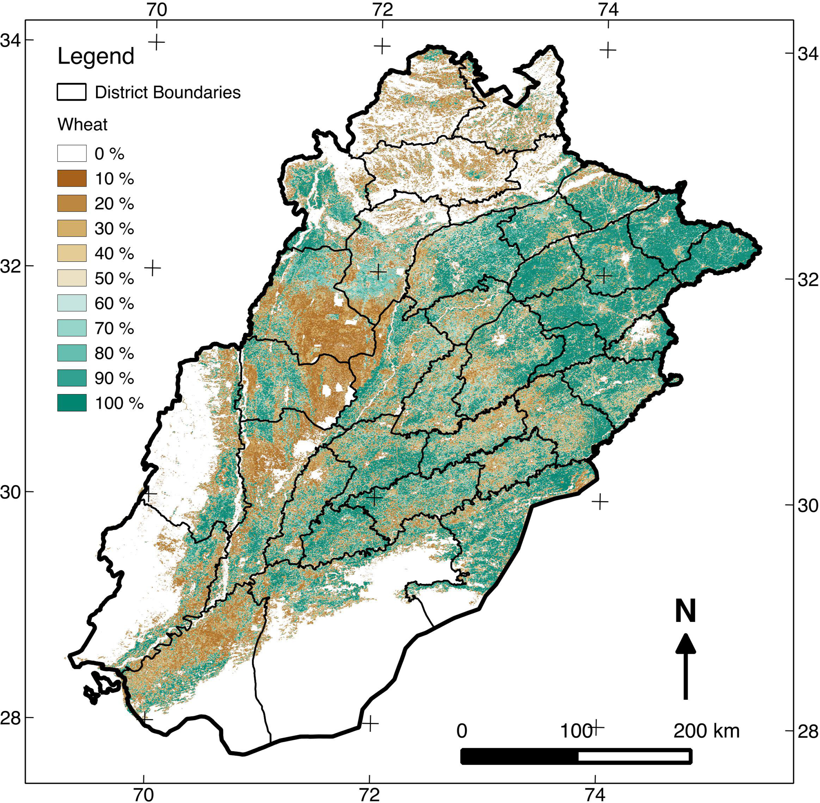
Figure 4 shows a map with the percent wheat estimate per pixel for Punjab Province for the latest Rabi season 2012/2013. Corresponding maps were calculated for all other years from 2001/2002 to 2011/2012. The absolute deviation of the MODIS-derived area estimates from reported values was between 0.4% and 6.8%, on average 2.4%. This result was slightly worse compared to simply taking the previous year’s reported area or the three-year or six-year moving average of previous years’ reported areas. We also tested the performance of the wheat yield and area estimates using the modified Nash–Sutcliffe efficiency index, E1, which is a global measure of model efficiency [50]. The E1 index for MODIS-derived versus reported wheat area for all years 2001/2002 to 2012/2013 was negative at −0.107, correspondingly. The index is defined as:
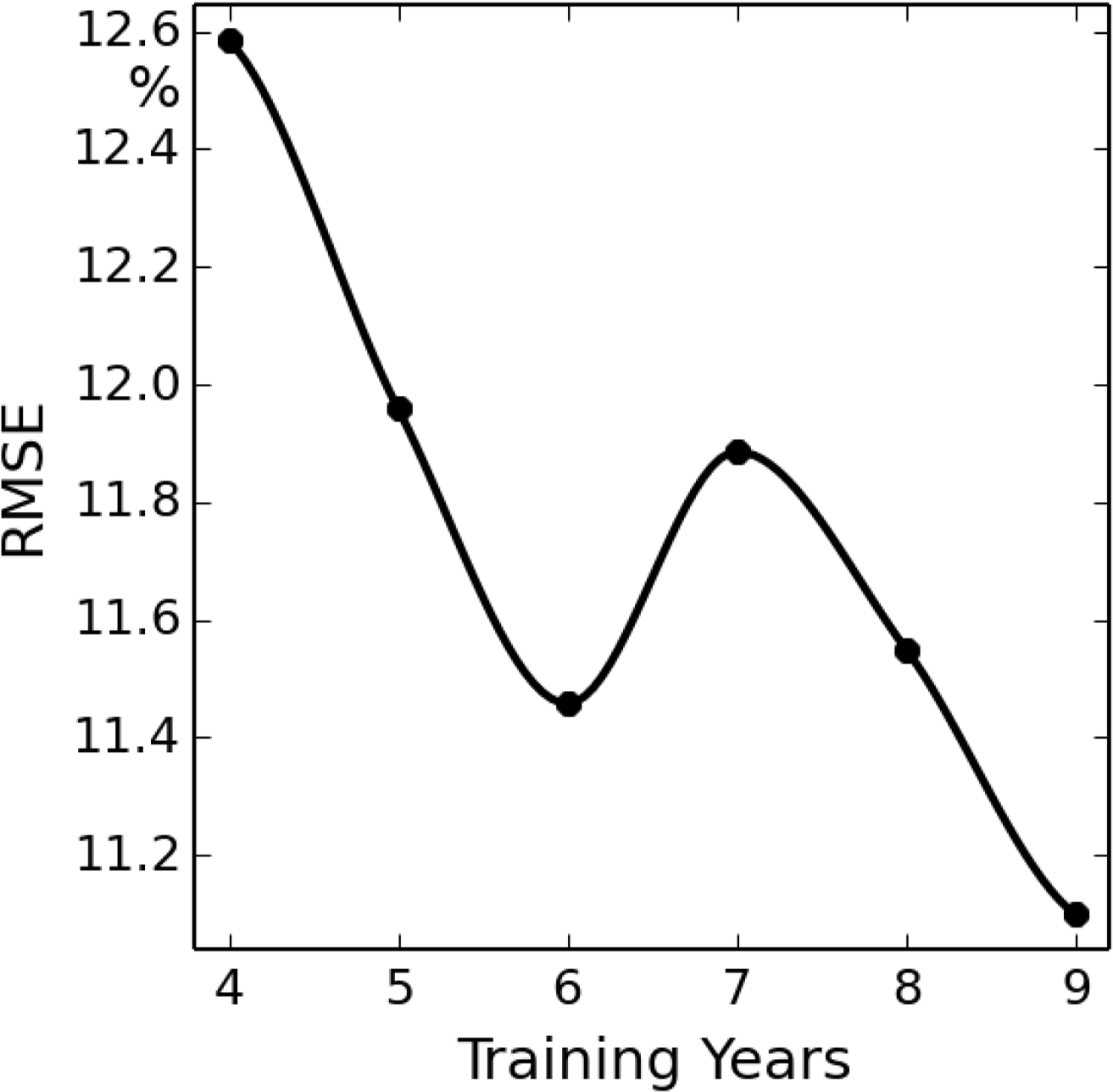
The optimal number of training years for yield forecasting was determined by calculating RMSE for the twelve Rabi seasons 2001/2002 to 2012/2013 using the WDRVI index and between four and nine training years. The RMSE reaches its minimum values at six and nine training years (Figure 5). Using nine training years results in an only slightly lower value (RMSE = 11.5%) compared to six years (RMSE = 11.1%). A main goal of this analysis is to identify the minimum data requirements for yield forecasting, and we therefore used six training years in the subsequent analysis.
The performance of four different vegetation indices, NDVI, SANDVI, EVI2 and WDRVI, for wheat yield forecasting was compared by calculating yield forecasts for all twelve Rabi seasons 2001/2002 to 2012/2013 on 18 February approximately six weeks before harvest. The forecasts were calculated at the district level using six years of training data. The VI values were derived from the 20% pixels per district with the highest percentage of wheat area. The total number of selected MODIS pixels per district ranged from 3626 to 35,451, on average 16,144. The results were compared with the final reported values published by the government in August of each year. At the district level, we calculated the root-mean-squared error (RMSE). At the provincial level, we calculated the relative deviation (difference in percent) of forecast versus reported yield. WDRVI resulted in the lowest RMSE, lower deviation than either NDVI or SANDVI and a tighter distribution around the mean than EVI2 (Figure 6). Absolute deviation of WDRVI-derived yield from reported values ranged from 0.2% in the 2007/2008 season to 11.5% in the 2011/2012 season.
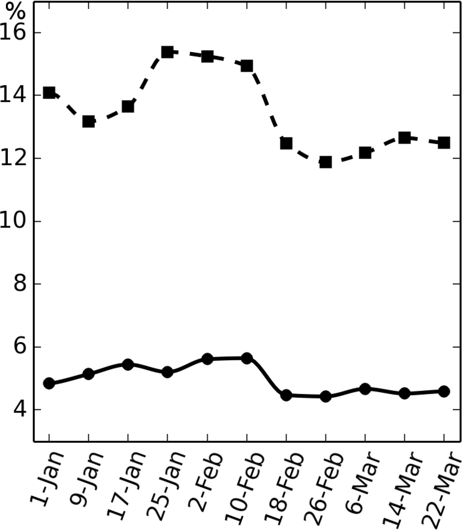
The best timing of the forecast during the course of the growing season was analyzed by forecasting yield at each eight-day time step using the WDRVI time series and six years of training data. Figure 7 shows the change over time of the RMSE and the deviation of forecast versus reported yield at the district level averaged over all 12 forecasting years. Average yield forecast accuracy was highest during the peak of the growing season approximately six weeks before harvest (18 February).
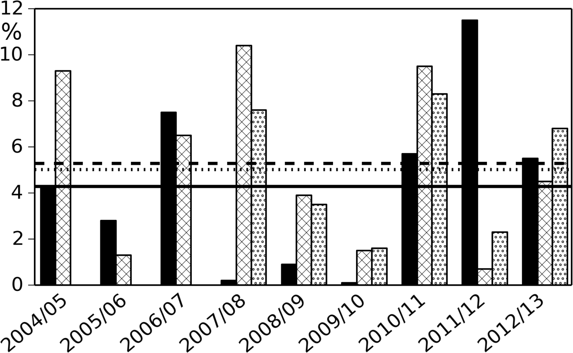
The yield forecasting results were compared to simply using the three-year or six-year moving averages of the years preceding the forecasting year (Figure 8). The results show that the forecast yields have, on average, a lower deviation from reported values than the moving averages, and thus, the forecast performs better. Correspondingly the modified Nash–Sutcliffe efficiency index (E1) is positive with E1 = 0.112.
5. Discussion
The purpose of this study was to develop a satellite-based system for wheat yield and production forecasting and to determine the data and processing requirements for a solution applicable to Punjab Province, Pakistan, but also transferable to other regions. Previous studies have shown the validity of using satellite-derived vegetation indices for wheat yield forecasting. Dempewolf et al. [32] achieved a higher agreement between forecast and reported yield for the 2011/2012 Rabi season using a similar methodology as employed in this study; however, it was based on NDVI only, used fewer training years, and when tested for other Rabi seasons, it performed significantly worse.
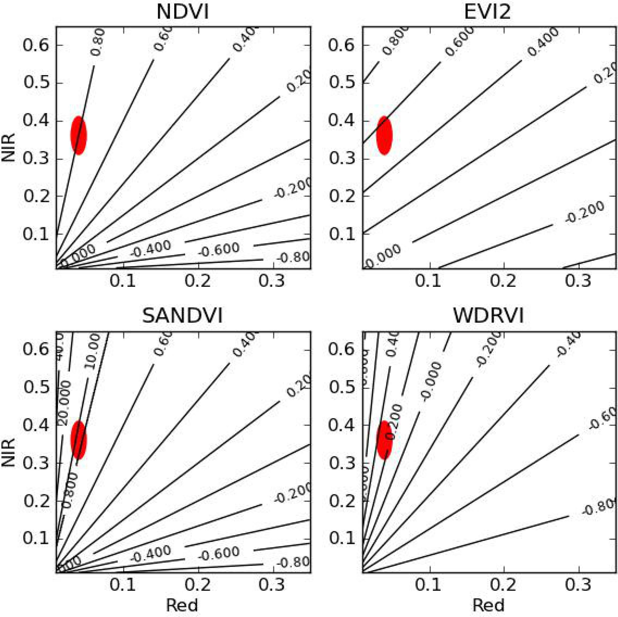
Our study confirms the usefulness of VIs in general and found an improvement in performance when using WDRVI compared to the other VIs. NDVI is known to saturate at high LAI values, and WDRVI was designed to improve the sensitivity of NDVI under these conditions. Figure 9 shows contour plots of NDVI, EVI2, SANDVI and WDRVI in the red/near-infrared reflectance two-dimensional space. The red ovals in the contour plots mark the typical ranges of red and near-infrared reflectance under high LAI conditions. In those areas, the number of iso-lines of each VI, and, thus, the sensitivity or resolution, is higher for WDRVI than the other indices, except SANDVI. The lower performance of the latter could be due to the fact that the index is not continuous and the density of contour lines increases suddenly at the artificial transition from NDVI to RVI.
The use of MODIS data for crop monitoring, particularly of agricultural fields at or below the MODIS spatial resolution, and the methodology of aggregating higher resolution Landsat imagery to the MODIS resolution are limited by the pixel purity of MODIS pixels. These effects are particularly relevant for off-nadir pixels with large viewing angles [51]. An analysis attributing error to MODIS geometries is an important next step, but requires a separate study and explicit spatial field data, which were not available for this analysis.
The results of this study allow one to make specific recommendations for the necessary number of training years. Six years of historical data were the minimum number of training years recommended for forecasting wheat yield. Fewer years did not seem to provide enough data points for deriving meaningful regression equations. The yield forecasting results compared positively to simpler methods of obtaining yield data, such as using the previous year’s value or the three-year or six-year moving average.
Wheat production forecasts depend on both the yield forecast and the satellite-derived wheat area estimates, combining two sources of uncertainty. The MODIS-derived area forecasts were, despite a regression adjustment, slightly less accurate than much simpler approaches, such as using the previous year’s value or the three-year or six-year moving average. This indicates that the 250-m resolution of MODIS data is not sufficient to map wheat area in the agricultural landscape of Pakistan. This is likely due to the fact that most agricultural fields do not cover an entire MODIS pixel, resulting in most pixels being mixed. Higher resolution satellite time series, such as Landsat 7 and 8, are therefore promising alternatives to determine the area of wheat and other crops.
The yield forecasts at the province level in general agreed well with reported values. It is important to keep in mind, however, that the reported values themselves have also an error associated with them. Forecasting results are expected to improve further together with advancements in field data collection and statistical methods used to produce the official reported values. The satellite-based yield forecasts were much less accurate for the 2011/2012 season than for other seasons. This might be due to unusual weather patterns in early 2012, when a prolonged cold spell in February 2012, delayed the normal development of the wheat crop [52]. However, due to more favorable conditions, the wheat crop caught up subsequently, and the final impact on yield was only small. This unusual pattern of delayed crop development during the normal seasonal peak time of wheat in mid-February in combination with a quick subsequent recovery might explain the lower performance of the forecasting system by the end of February in the 2011/2012 Rabi season.
6. Conclusions
This study provides a basis for designing and developing a comprehensive, operationally viable wheat yield forecasting system with high accuracy using the example of Punjab Province, Pakistan. The results of this analysis are based on a limited number of training years and on a single wheat growing region. The approach needs to be evaluated further for more years as new data become available and for other regions. The methodology requires six years of historic reported yield statistics at the district or comparable administrative level and satellite data for the six preceding years plus the current year. The necessary MODIS and Landsat satellite data inputs are readily and freely available. The ideal number of training years may vary for different regions. The methodology is limited by the fact that MODIS satellite observations are at comparatively coarse spatial resolution relative to the distribution of field sizes. Furthermore, optical satellite data are also prone to negative effects of cloud cover, which might reduce the feasibility of transferring the methodology to other, more cloud-prone regions. Low cloud cover during the wheat growing season was an advantage for this study conducted in Pakistan. The next steps are to test the use of a wall-to-wall Landsat time series classification for producing wheat area estimates at higher spatial resolution and testing the yield and production forecasting system in other wheat growing regions. Crop analysts of national and international agencies can use these data as one important source of information for making assessments of current crop conditions and yield and production forecasts. This has potential use for crop market outlooks, food security assessments, food price forecasts and regional and global monitoring systems.
Acknowledgments
We would like to thank the Crop Reporting Service of the Government of Punjab, Pakistan, for contributing crop statistical data and the United States Department of Agriculture for funding and support. We thank William H. Wigton for his thoughtful review and comments on the manuscript.
Author Contributions
Jan Dempewolf developed the yield model, conducted the overall analysis and led the writing of the manuscript; Bernard Adusei processed the MODIS data and produced the percent wheat data layers; Inbal Becker-Reshef provided advice and expertise for creating the wheat yield model and data analysis; Matthew Hansen provided guidance and advice on creating the MODIS metrics and percent wheat data layers; Peter Potapov developed the application for mapping wheat using time-series Landsat images; Ahmad Khan classified Landsat data for wheat used for training and contributed local expert knowledge; Brian Barker classified Landsat data for wheat.
Conflicts of Interest
The authors declare no conflicts of interest.
References
- Worldbank. Health Nutrition and Population Statistics. Available online: http://databank.worldbank.org (accessed on 24 September 2014).
- Briscoe, J.; Qamar, U. Pakistan’s Water Economy: Running Dry; Oxford University Press: Karachi, Pakistan, 2005. [Google Scholar]
- Khan, S.B.; Khattak, A.; Hafeezullah; Rehman, A. Agricultural Statistics of Pakistan 2010–2011; Pakistan Bureau of Statistics, Government of Pakistan: Islamabad, Pakistan, 2012. [Google Scholar]
- Ministry of Finance of the Government of Pakistan. Pakistan Economic Survey 2011–2012. Available online: http://www.finance.gov.pk/survey_1112.html (accessed on 24 September 2014).
- Dorosh, P.; Salam, A. Wheat markets and price stabilisation in Pakistan: An analysis of policy options. Pak. Dev. Rev 2008, 47, 71–87. [Google Scholar]
- Niaz, M.S. Wheat Policy—A Success or Failure. DAWN. Available online: http://www.dawn.com/news/194423/wheat-policy-a-success-or-failure/ (accessed on 24 September 2014).
- Akhtar, I.U.H. Pakistan Needs a New Crop Forecasting System. Available online: http://www.scidev.net/en/new-technologies/space-technology/opinions/pakistan-needs-a-new-crop-forecasting-system.html (accessed on 24 September 2014).
- Bauer, M.E. The role of remote sensing in determining the distribution and yield of crops. Adv. Agron 1975, 27, 271–304. [Google Scholar]
- Erickson, J.D. The LACIE experiment in satellite aided monitoring of global crop production. In The Role of Terrestrial Vegetation in the Global Carbon Cycle: Measurement by Remote Sensing; John Wiley: Chichester, UK, 1984; pp. 191–217. [Google Scholar]
- Doraiswamy, P.; Hodges, T.; Phinney, D. Crop Yield Literature Review for AgRISTARS Crops Corn, Soybeans, Wheat, Barley, Sorghum, Rice, Cotton, and Sunflowers; Technical Report 73–312; Lockheed Electronics Co.: Houston, UK, 1979. [Google Scholar]
- Baruth, B.; Royer, A.; Klisch, A.; Genovese, G. The use of remote sensing within the MARS crop yield monitoring system of the European Commission. Int. Arch. Photogramm. Remote Sens. Spat. Inf. Sci 2008, 37, 935–940. [Google Scholar]
- Becker-Reshef, I.; Justice, C.; Sullivan, M.; Vermote, E.; Tucker, C.; Anyamba, A.; Small, J.; Pak, E.; Masuoka, E.; Schmaltz, J. Monitoring global croplands with coarse resolution earth observations: The Global Agriculture Monitoring (GLAM) project. Remote Sens 2010, 2, 1589–1609. [Google Scholar]
- Bastiaanssen, W.G.; Ali, S. A new crop yield forecasting model based on satellite measurements applied across the Indus Basin, Pakistan. Agric. Ecosyst. Environ 2003, 94, 321–340. [Google Scholar]
- SUPARCO. Crop Situation Forecast. Available online: http://www.suparco.gov.pk/pages/pak-scms.asp (accessed on 24 September 2014).
- Pittman, K.; Hansen, M.C.; Becker-Reshef, I.; Potapov, P.V.; Justice, C.O. Estimating global cropland extent with multi-year MODIS data. Remote Sens 2010, 2, 1844–1863. [Google Scholar]
- Breiman, L. Bagging predictors. Mach. Learn 1996, 24, 123–140. [Google Scholar]
- DeFries, R.; Hansen, M.; Townshend, J. Global discrimination of land cover types from metrics derived from AVHRR pathfinder data. Remote Sens. Environ 1995, 54, 209–222. [Google Scholar]
- Hansen, M.C.; DeFries, R.S.; Townshend, J.R.; Sohlberg, R.; Dimiceli, C.; Carroll, M. Towards an operational MODIS continuous field of percent tree cover algorithm: Examples using AVHRR and MODIS data. Remote Sens. Environ 2002, 83, 303–319. [Google Scholar]
- Potapov, P.V.; Turubanova, S.A.; Hansen, M.C.; Adusei, B.; Broich, M.; Altstatt, A.; Mane, L.; Justice, C.O. Quantifying forest cover loss in Democratic Republic of the Congo, 2000–2010, with Landsat ETM+ data. Remote Sens. Environ 2012, 122, 106–116. [Google Scholar]
- Lobell, D.B.; Asner, G.P. Cropland distributions from temporal unmixing of MODIS data. Remote Sens. Environ 2004, 93, 412–422. [Google Scholar]
- Ozdogan, M. The spatial distribution of crop types from MODIS data: Temporal unmixing using Independent Component Analysis. Remote Sens. Environ 2010, 114, 1190–1204. [Google Scholar]
- Wardlow, B.D.; Egbert, S.L. Large-area crop mapping using time-series MODIS 250 m NDVI data: An assessment for the U.S. Central Great Plains. Remote Sens. Environ 2008, 112, 1096–1116. [Google Scholar]
- Chang, J.; Hansen, M.C.; Pittman, K.; Carroll, M.; DiMiceli, C. Corn and soybean mapping in the United States using MODIS time-series data sets. Agron. J 2007, 99, 1654–1664. [Google Scholar]
- Becker-Reshef, I.; Vermote, E.; Lindeman, M.; Justice, C. A generalized regression-based model for forecasting winter wheat yields in Kansas and Ukraine using MODIS data. Remote Sens. Environ 2010, 114, 1312–1323. [Google Scholar]
- Gosal, G. Physical geography of the punjab. J. Punjab Stud 2004, 11, 19–37. [Google Scholar]
- Hijmans, R.; Cameron, S.; Parra, J.; Jones, P.; Jarvis, A. Very high resolution interpolated climate surfaces for global land areas. Int. J. Climatol 2005, 25, 1965–1978. [Google Scholar]
- Steduto, P.; Hsiao, T.; Fereres, E.; Raes, D. Crop Yield Response to Water; Technical Report 66; FAO: Rome, Italy, 2012. [Google Scholar]
- FAO, Punjab CRS: Base Line Survey—Agriculture Information System; Technical Report; FAO/UN SUPARCO: Rome, Italy, 2012.
- Tucker, C.J.; Holben, B.N.; Elgin, J.H., Jr.; McMurtrey, J.E., III. Remote sensing of total dry-matter accumulation in winter wheat. Remote Sens. Environ 1981, 11, 171–189. [Google Scholar]
- Labus, M.P.; Nielsen, G.A.; Lawrence, R.L.; Engel, R.; Long, D.S. Wheat yield estimates using multi-temporal NDVI satellite imagery. Int. J. Remote Sens 2002, 23, 4169–4180. [Google Scholar]
- Mkhabela, M.; Bullock, P.; Raj, S.; Wang, S.; Yang, Y. Crop yield forecasting on the Canadian Prairies using MODIS NDVI data. Agric. For. Meteorol 2011, 151, 385–393. [Google Scholar]
- Dempewolf, J.; Adusei, B.; Becker-Reshef, I.; Barker, B.; Potapov, P.; Hansen, M.; Justice, C. Wheat production forecasting for Pakistan from satellite data. In Proceedings of 2013 IEEE Internationa Geoscience and Remote Sensing Symposium (IGARSS), Melbourne, VIC, Australia, 21–26 July 2013; pp. 3239–3242.
- Ren, J.; Chen, Z.; Zhou, Q.; Tang, H. Regional yield estimation for winter wheat with MODIS-NDVI data in Shandong, China. Int. J. Appl. Earth Obs. Geoinf 2008, 10, 403–413. [Google Scholar]
- Meroni, M.; Marinho, E.; Sghaier, N.; Verstrate, M.; Leo, O. Remote sensing based yield estimation in a stochastic framework—Case study of durum wheat in Tunisia. Remote Sens 2013, 5, 539–557. [Google Scholar]
- Funk, C.; Budde, M.E. Phenologically-tuned MODIS NDVI-based production anomaly estimates for Zimbabwe. Remote Sens. Environ 2009, 113, 115–125. [Google Scholar]
- Tucker, C.J. Red and photographic infrared linear combinations for monitoring vegetation. Remote Sens. Environ 1979, 8, 127–150. [Google Scholar]
- Gu, Y.; Wylie, B.K.; Howard, D.M.; Phuyal, K.P.; Ji, L. NDVI saturation adjustment: A new approach for improving cropland performance estimates in the Greater Platte River Basin, USA. Ecol. Indic 2013, 30, 1–6. [Google Scholar]
- Huete, A.R.; Liu, H.Q.; Batchily, K.; Van Leeuwen, W. A comparison of vegetation indices over a global set of TM images for EOS-MODIS. Remote Sens. Environ 1997, 59, 440–451. [Google Scholar]
- Gao, X.; Huete, A.R.; Ni, W.G.; Miura, T. Optical-biophysical relationships of vegetation spectra without background contamination. Remote Sens. Environ 2000, 74, 609–620. [Google Scholar]
- Jiang, Z.; Huete, A.; Didan, K.; Miura, T. Development of a two-band enhanced vegetation index without a blue band. Remote Sens. Environ 2008, 112, 3833–3845. [Google Scholar]
- Gitelson, A.A. Wide dynamic range vegetation index for remote quantification of biophysical characteristics of vegetation. J. Plant Physiol 2004, 161, 165–173. [Google Scholar]
- Gitelson, A.A.; Wardlow, B.D.; Keydan, G.P.; Leavitt, B. An evaluation of MODIS 250-m data for green LAI estimation in crops. Geophys. Res. Lett 2007. [Google Scholar] [CrossRef]
- Guindin-Garcia, N.; Gitelson, A.A.; Arkebauer, T.J.; Shanahan, J.; Weiss, A. An evaluation of MODIS 8- and 16-day composite products for monitoring maize green leaf area index. Agric. Forest Meteorol 2012, 161, 15–25. [Google Scholar]
- Sakamoto, T.; Gitelson, A.A.; Arkebauer, T.J. MODIS-based corn grain yield estimation model incorporating crop phenology information. Remote Sens. Environ 2013, 131, 215–231. [Google Scholar]
- Sibley, A.M.; Grassini, P.; Thomas, N.E.; Cassman, K.G.; Lobell, D.B. Testing remote sensing approaches for assessing yield variability among maize fields. Agron. J 2014, 106, 24–32. [Google Scholar]
- Boken, V.K.; Shaykewich, C.F. Improving an operational wheat yield model using phenological phase-based Normalized Difference Vegetation Index. Int. J. Remote Sens 2002, 23, 4155–4168. [Google Scholar]
- Basnyat, P.; McConkey, B.; Lafond, G.P.; Moulin, A.; Pelcat, Y. Optimal time for remote sensing to relate to crop grain yield on the Canadian prairies. Can. J. Plant Sci 2004, 84, 97–103. [Google Scholar]
- Carfagna, E.; Gallego, F.J. Using remote sensing for agricultural statistics. Int. Stat. Rev 2005, 73, 389–404. [Google Scholar]
- Johnson, D.; Mueller, R. The 2009 cropland data layer. Photogramm. Eng. Remote Sens 2010, 76, 1201–1205. [Google Scholar]
- Krause, P.; Boyle, D.P.; Bäse, F. Comparison of different efficiency criteria for hydrological model assessment. Adv. Geosci 2005, 5, 89–97. [Google Scholar]
- Duveiller, G.; Baret, F.; Defourny, P. Crop specific green area index retrieval from MODIS data at regional scale by controlling pixel-target adequacy. Remote Sens. Environ 2011, 115, 2686–2701. [Google Scholar]
- SUPARCO, PAK-SCMS Bulletin—Pakistan Satellite Based Crop Monitoring System; Monthly Bulletin Volume II, Issue 3; Government of Pakistan—SUPARCO, UN-FAO: Islamabad, Pakistan, 2012.


| Year | Path/Row | Early GS | Height GS | Harvest S |
|---|---|---|---|---|
| 2001/2002 | 150/037 | 2001312 | 2002043 | 2002139 |
| 150/039 | 2001344 | 2002043 | 2002139 | |
| 2002/2003 | 150/037 | 2002363 | 2003078 | 2003126 |
| 150/039 | 2002363 | 2003078 | 2003126 | |
| 2003/2004 | 150/037 | 2003350 | 2004033 | 2004145 |
| 150/039 | 2003334 | 2004065 | 2004145 | |
| 2004/2005 | 150/037 | 2005019 | 2005083 | 2005131 |
| 150/039 | 2005019 | 2005051 | 2005131 | |
| 2005/2006 | 150/037 | 2006006 | 2006070 | 2006118 |
| 150/039 | 2006006 | 2006070 | 2006118 | |
| 2006/2007 | 150/037 | 2007025 | 2007073 | 2007137 |
| 150/039 | 2007009 | 2007073 | 2007137 | |
| 2007/2008 | 150/037 | 2008044 | 2008060 | 2008124 |
| 150/039 | 2008028 | 2008060 | 2008108 | |
| 2008/2009 | 150/037 | 2009030 | 2009070 | 2009110 |
| 150/039 | 2009014 | 2009062 | 2009126 | |
| 2009/2010 | 150/037 | 2010033 | 2010073 | 2010113 |
| 150/039 | 2010033 | 2010057 | 2010113 |
| Bit | Bit Combination | Description |
|---|---|---|
| 0–1 | 01, 10 | Cloudy, mixed cloudy |
| 2 | 1 | Cloud shadow |
| 3–5 | 000, 010, 011, 100, 101, 110, 111 | Water surfaces |
| 6–7 | 11 | High aerosol |
| 8–9 | 01, 10, 11 | Cirrus clouds |
| 10 | 1 | Cloudy (internal flag) |
| 11 | 1 | Fire |
| 12 | 1 | Snow/Ice |
| 13 | 1 | Adjacent to cloud |
| R | NIR | SWIR | Th | NDVI | NDWI | |
|---|---|---|---|---|---|---|
| R | × | × | × | × | ||
| NIR | × | × | × | × | ||
| SWIR | × | × | × | × | ||
| Th | × | × | × | |||
| NDVI | × | × | × | |||
| NDWI | × | × | × |
© 2014 by the authors; licensee MDPI, Basel, Switzerland This article is an open access article distributed under the terms and conditions of the Creative Commons Attribution license (http://creativecommons.org/licenses/by/4.0/).
Share and Cite
Dempewolf, J.; Adusei, B.; Becker-Reshef, I.; Hansen, M.; Potapov, P.; Khan, A.; Barker, B. Wheat Yield Forecasting for Punjab Province from Vegetation Index Time Series and Historic Crop Statistics. Remote Sens. 2014, 6, 9653-9675. https://0-doi-org.brum.beds.ac.uk/10.3390/rs6109653
Dempewolf J, Adusei B, Becker-Reshef I, Hansen M, Potapov P, Khan A, Barker B. Wheat Yield Forecasting for Punjab Province from Vegetation Index Time Series and Historic Crop Statistics. Remote Sensing. 2014; 6(10):9653-9675. https://0-doi-org.brum.beds.ac.uk/10.3390/rs6109653
Chicago/Turabian StyleDempewolf, Jan, Bernard Adusei, Inbal Becker-Reshef, Matthew Hansen, Peter Potapov, Ahmad Khan, and Brian Barker. 2014. "Wheat Yield Forecasting for Punjab Province from Vegetation Index Time Series and Historic Crop Statistics" Remote Sensing 6, no. 10: 9653-9675. https://0-doi-org.brum.beds.ac.uk/10.3390/rs6109653