1. Introduction
The power system in Finland consists of power plants, a nationwide transmission grid, regional networks, distribution networks and electricity consumers. It is part of the inter-Nordic power system together with the systems in Sweden, Norway and Eastern Denmark and is also connected to the Russian and Estonian networks. High-voltage power lines are used in the transmission grid to compensate for the long transmission distances and to reduce electricity transmission losses. Regional networks are connected to the nationwide grid and distribute electricity regionally. Households are linked to regional distribution networks. In Finland alone, 119,661 km of regional networks exist with more than 70,000 km located inside forests. In Finland, the length of power lines surrounded by forest exceeding 13 m in height totals approximately 35,000 km. The number of low voltage networks linking households to the regional networks is estimated to be 23,500 km. High-voltage power lines, i.e., the nationwide transmission grid, can be quite easily mapped using laser scanning data, because vegetation close to high-voltage lines is typically removed and also because the power lines are located higher off the ground, in contrast to regional networks and lower voltage networks. Lower voltage power lines are located in the middle of dense forests, and it is difficult to classify power lines from such environments.
Over the past decades, power lines have been documented mainly by aerial images manually or in a semi-automated manner (e.g., stereo-images) [
1]. However, measurements based on aerial images are visual dependent. For open areas, when power lines are visible from aerial images, the measurement is easy. However, in forest areas, a large number of trees in the surroundings will interfere with visual recognition. In many cases, power lines in forest areas are not visible from aerial images. Therefore, it is fairly challenging to visually measure the power lines from images. Since the advent of commercial airborne laser scanning (ALS), research has revealed that surveying and modelling electric power lines are suitable for laser scanning application [
2]. By using the ALS data, objects with small diameters (such as power-line cables) can yield dense, rapid and accurate measurements [
3]. Since 1995, thousands of kilometers of power-lines have already been mapped by ALS [
4]. However, labor-intensive data manipulation still plays a primary role in today’s practice [
5]. Fully-automated solutions are needed.
With the advancement of sensor technology, the ALS point density has recently increased from a few points per m
2 to the current data density of approximately 55 points per m
2. The objects’ levels of detail are markedly different according to the point density variation. Many classification methodologies have been developed according to different point densities. For example, Axelsson (1999) [
2] utilized ALS data with a density of eight points/m
2 for power line detection. He presented a classification method of power lines by looking for parallel and linear 2D structures based on the Hough transformation method and utilizing a 2D line equation for line extraction. Melzer and Briese (2004) [
3] proposed a method for power line extraction and modelling from ALS by using 2D Hough transformation and 3D catenary curve fitting methods. The density of ALS data was at that time up to 10 points/m
2. Clode and Rottensteiner (2005) [
6] detected trees and power lines from less than one point per m
2 point cloud in Sydney. First and last pulse return differences were applied. McLaughlin (2006) [
7] used ALS data with an average point spacing of 1.2 m–2.4 m on a power line. Based on these data, he presented a supervised method to classify the power lines. Liu
et al. (2009) [
8] detected power lines with a 2D gray-level image, the intensity of laser return and an improved Hough transform. Jwa
et al. (2009) [
9] introduced a voxel-based piecewise line detector (VPLD) approach for automatic power line reconstruction using a density of five points/m
2 ALS data. Liang
et al. (2011) [
10] used the random sample consensus (RANSAC) method to determine which points belong to a line. Kim and Sohn (2011) [
11] used RANSAC, minimum description length and principal component analysis in feature extraction and random forests as a classification technique for a test dataset with a density of 30 points per m
2. Sohn
et al. (2012) [
12] proposed that using a Markov random field (MRF) classifier would delineate the spatial context of linear and planar features, as in a graphical model for power line and building classification. The test data were at a density of 16 points/m
2. Kim and Sohn (2013) [
5] proposed a point-based supervised random forest method for five utility corridor object classification from an ALS point cloud set with a density of 25–30 points/m
2. Based on the above literature review, the methods for power line detection can be summarized into two types: line-shape-based detection methods (e.g., RANSAC and 2D Hough transformation [
2,
3,
8,
10,
13]) and supervised classification methods [
7,
9,
11,
12]. Line-shape-based detection methods incur a relatively high computational cost, especially for a large area dataset. Each point must be calculated to determine whether it belongs to a line. Therefore, some researchers [
9,
14] have proposed piece-wise line detection to improve the efficiency. However, because the detected results are usually pieces of lines, the correct topographic relations must be calculated between the turn points. For supervised classification methods, a large training dataset is required to achieve the desired results. In addition, unbalance sampling will lead to an increased rate of misclassification.
A recent study utilizing mobile laser scanning (MLS) for corridor mapping is highly relevant. The publications concerning mobile laser scanning include building wall extraction [
15], pole extraction [
16], road environment modelling [
17,
18], street object classification [
19] and power line extraction [
20]. The suitability of object extraction from both ALS and MLS was proposed in Zhu and Hyyppä [
21]. With regard to power line extraction, MLS is suitable for small-area, but detailed mapping. A high computational cost is incurred for larger area mapping due to the high point density from MLS. However, ALS not only can cover a large area, but also is suitable for undulating terrains (e.g., hills or mountains) that are difficult to reach using ground-based vehicles. In the latest study for power line extraction for an urban corridor environment from MLS data, Cheng
et al. (2014) [
20] presented a method comprised of three steps: extracting power line points using a voxel-based hierarchical method, a bottom-up single power line point clustering and 3D power line fitting. The method was based on detecting the power line points and grouping them together.
In previous research, power line detection in the forest environment is rare due to the difficulties in such an environment. In this paper, we propose a novel approach to solve the problem of classifying the power lines in a forest environment. This method is based on two different technologies: statistical analysis for data pre-processing and image-based processing technology for data classification. Statistical analysis selects the potential power line candidates using certain statistical criteria (
i.e., height criteria, density criteria and histogram analysis), and then, a large number of unrelated points are removed. After obtaining the candidates for power lines, these points are transferred to a binary image. Image processing technologies are employed for noise removal and feature extraction. The 2D power line image is transferred to 3D by using the same parameters as in the previous step: 3D points to a binary image. Thus, 3D power lines are extracted. In the following sections, our paper is organized as follows: In
Section 2, materials used in this paper will be introduced, and our methods will be described in detail. The following section presents the results from six ALS datasets located in different forest areas. In this section, the advantages and disadvantages of the methods will also be discussed and future issues will be considered. The last section contains the conclusions.
2. Materials and Methods
2.1. Data Resources and Test Fields
The data resources include six sets of ALS point clouds and six sets of reference data for quality analysis. All datasets were acquired from Kirkkonummi, Finland, with a density of 55 points per m2. These point clouds contain georeferenced 3D coordinates (X, Y and Z) in an ETRS-TM35FIN coordinate system: X towards the east, Y referring to the north and Z upwards.
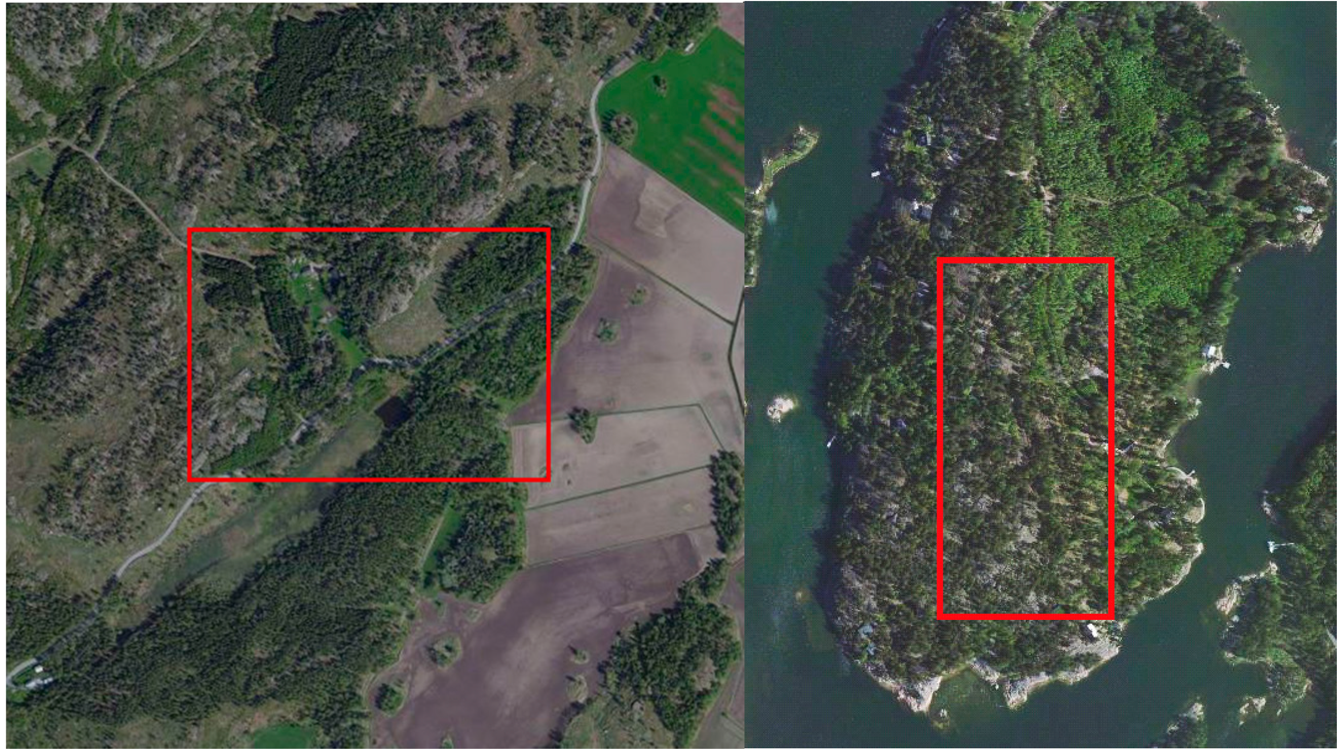
Our study areas are covered by large areas of forests (see
Figure 1). Each of the six datasets covers an area varying from 200 × 300 m
2 to 300 × 500 m
2.
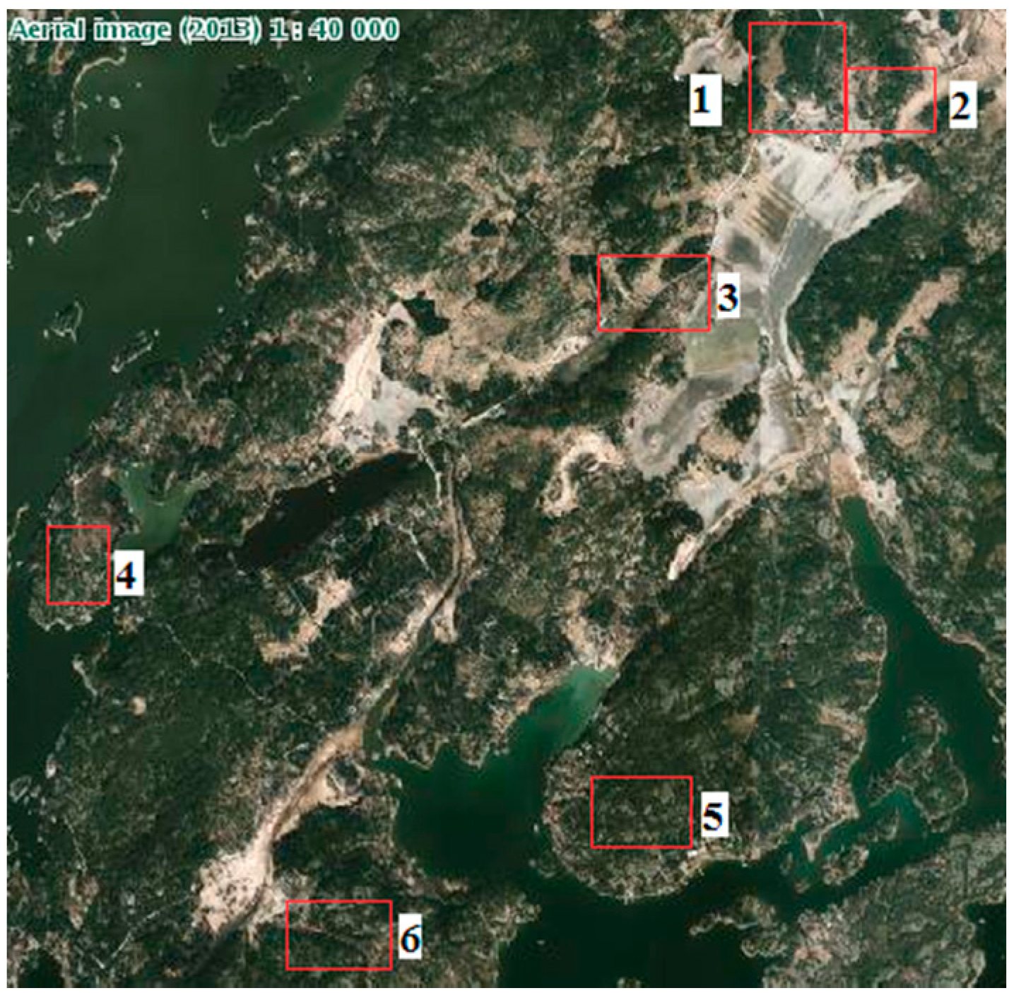
Figure 2 displays the locations of the six study areas on a 1:40,000 topographic map. The two areas indicated in red in
Figure 1 represent Areas 3 and 4 in
Figure 2.
Figure 1.
Examples of the test areas (with red marks) in Kirkkonummi.
Figure 1.
Examples of the test areas (with red marks) in Kirkkonummi.
Figure 2.
Illustration of the study areas on an aerial image (from the Finnish National Land Survey). The numbers on the map indicate the IDs of the test fields.
Figure 2.
Illustration of the study areas on an aerial image (from the Finnish National Land Survey). The numbers on the map indicate the IDs of the test fields.
2.2. Methods
Our algorithm was based on two main steps: (i) statistical analysis; and (ii) image-based processing. The aim of the statistical analysis was to identify candidates for the power lines among the dense point cloud. The criteria for power line candidate selection (e.g., height criteria, density criteria and histogram thresholds) were defined. After the selection of candidates, cutoff edges on both sides of the power lines were clear and visible. The follow-up work is image-based processing. Image-based processing involves 2D recognition processing. The height information is not presented from 3D to 2D. In 2D space, objects were separated by their 2D geometric properties, for example the area size of an object, the shape of an object and the length and width of an object. For example, from the top view, individual trees usually have round shapes, buildings have block-like shapes and power lines have shapes that are close to linear. However, these properties are usually not clear when multiple objects are close to each other. Therefore, it is difficult to directly separate the different objects by their shapes. Multiple geometric criteria, such as the major and minor lengths of an object and the size of its area, are needed.
Figure 3 illustrates the workflow of our method. In this figure, the statistical analysis steps are contained within the red dashed lines, whereas the image-based processing steps are displayed within the green dashed lines.
Figure 3.
Method for power line extraction. Red frame: steps in the statistical analysis; green frame: steps in the image-based processing.
Figure 3.
Method for power line extraction. Red frame: steps in the statistical analysis; green frame: steps in the image-based processing.
In this paper, data processing is conducted at three different levels: (i) an entire dataset; (ii) a grid; and (iii) a bin in a grid. An entire dataset can be gridded into m × n grids. A grid can create equally spaced bins according to their heights by using the histogram method. Each bin is called a bin in a grid.
Algorithm 1 addresses the process of power line extraction. A list of abbreviations shows in
Table 1. It was developed based on the assumption that the point density of the dataset is not less than 20 points per m
2. Algorithm 1 is divided into three parts: statistical analysis (Steps 1, 2 and 3), image analysis (Steps 4 and 5) and power line extraction (Step 6). Statistical analysis aims to identify power line candidates.
Table 2 lists the European regulations regarding power line overhead heights. It can be observed that the minimum heights of power lines above the ground vary according to the voltages. However, the minimum height cannot be less than 5.2 m. Considering the possible curvatures and ages of the power lines (possibly not completely vertical to the ground), we set a height threshold above ground (Ht = 4 m) to separate the data into two sectors. This separation was performed by gridding the data in the xy plane and, from each grid, extracting the points that are 4 m higher than or equal to the ground ({Pij} ∈ Pu). The rest of the data are in group Pl. The power line candidates are selected from the point set “Pu”. The selection standards of the candidates are as follows:
(i) Height criteria. In a grid, if the height difference is less than one-half meter, all points in the grid are selected as candidates. This threshold was set according to the possible curvature of the power lines.
(ii) Density distribution. For example, in a grid, e.g., 1 × 1 m2, when the number of power line points is smaller than the square root of 2 × the density of the points, they are selected as power lines. That is, the candidate points are distributed along the diagonal of a square.
Table 1.
A list of abbreviations.
Table 1.
A list of abbreviations.
| Abbreviation | Description |
|---|
| P(x, y, z) | 3D point cloud; |
| Pij | A set of point in a grid (i, j), with 3D coordinates (Xij, Yij, Zij); |
| Plij | A set of point lower than a certain height threshold; |
| Puij | A set of point in a grid (i, j) greater than or equal to a certain height threshold; |
| Zmin | The minimum height value in a grid; each grid has its minimum height; |
| Ht | The height threshold for the lowest power line in a regulation; |
| numOfPoints_g | The number of the points in a grid; |
| Pdensity | The density of a point cloud, points/m2; |
| Zbij | The height value of a point in a bin (produced by a height histogram) of a grid (i, j); |
| Zbmin | The minimum height value of a point in a bin of a grid (i, j); |
| numOfPoints_b | The number points in a bin; |
| Pbij | The points in a bin of a grid (i, j); |
| paraArea_min | The minimum area of a single region of a binary image that can be considered a power line; |
| paraArea_max | The maximum area of a single region of a binary image that can be considered a power line; |
| paraLength | The length of the major axis of one region in a binary image; |
| paraShape | Eccentricity of a single region in a binary image, which means that “1” is a line and “0” is a circle; |
| sizeP | Pixel size of a binary image. |
| Algorithm 1 Power Line Detection |
| 1: Grid the dataset {P(x, y, z)}, e.g., grid = 1 m * 1 m. {P} = {P11} + {P12} + {P13} +...... + {Pij} |
| 2: {Pij} ={Plij} + {Puij}, where Pij (Zij − Zmin < Ht) ∈ Plij, Pij (Zij − Zmin >= Ht) ∈ Puij |
| 3: Power line candidate points are selected from {Puij} |
| if (Zij − Zmin <= 0.5) | (numOfPoints_g <= sqrt (2 * Pdensity)), then |
| Pij∈ {candidates}, |
| else |
| if Zij − Zmin > 0.5, then |
| using histogram analyzing the height distribution with (for example) a 1 m interval, {Pij} = {bin} |
| if only one bin has points, the others are empty, then |
| Pbij ∈ {candidates}, |
| else |
| if (Zbij −Zbmin <= 0.5) & (numOfPoints_b >= sqrt (Pdensity)), then |
| Pbij (Zbij − Zbmin <= 0.5) ∈ {candidates}, |
| end if |
| end if |
| end if |
| end if |
| 4: Transfer {candidates} to a raster image I(m,n) by using their X, Y coordinates and predefined |
| if a raster is not empty, then |
| it is set to 1 |
| else it is set to 0 |
| end if |
| 5: Image regions are labelled: I = R1+R2+R3+......+Rk, where R1, R2, R3,.... Rk are the labelled image regions |
| if area of Rk > paraArea_min & area of Rk <= paraArea_max & length of major axis of Rk > paraLength |
| & Eccentricity of Rk > paraShape, then |
| accepts as {2Dpower lines} |
| end if |
| 6: Transfer {2Dpower lines} to {3Dpower lines} by reverse processing of step (4) |
Table 2.
Regulations for the heights of power lines [
22].
Table 2.
Regulations for the heights of power lines [22].
| | Schedule 2
Minimum Height Above Ground of Overhead Lines | Regulation 17 (2) |
|---|
| Column 1 | Column 2 | Column 3 |
| Nominal Voltages | Over Roads | Other Locations |
| Not exceeding 33,000 volts | 5.8 meters | 5.2 meters |
| Exceeding 33,000 volts, but not exceeding 66,000 volts | 6 meters | 6 meters |
| Exceeding 66,000 volts, but not exceeding 132,000 volts | 6.7 meters | 6.7 meters |
| Exceeding 132,000 volts, but not exceeding 275,000 volts | 7 meters | 7 meters |
| Exceeding 275,000 volts, but not exceeding 400,000 volts | 7.3 meters | 7.3 meters |
Histogram analysis. If the height difference in a grid is greater than one-half meter, this means that tree points or multiple objects are present in this grid. We use a histogram to perform the height analysis. For example, in a grid with a height difference of 10 m, we may set each bin equal to 1 m (an interval size in a histogram). Then, for each grid, if only one bin contains points, all points in that grid are selected as candidates. Alternatively, for each bin, if the height difference is less than one-half meter and the number of points is not less than the square root of the point density, we select all points in that bin as candidates.
After candidate selection, all candidate points are gridded into a binary image. Image regions can be separated according to the power line characteristics, e.g., the continuity and the shape. Continuity means that the image contains a large area of points, whereas the shape of an image region can be determined by the following parameters: area size, eccentricity and major and minor lengths. We utilize these properties to separate power lines from the other objects. The separated 2D power lines (a binary image) were transferred back to 3D points using the same settings (e.g., raster size and the maximum and minimum X and Y coordinates) as were used when the 3D candidates were transferred to a binary image.
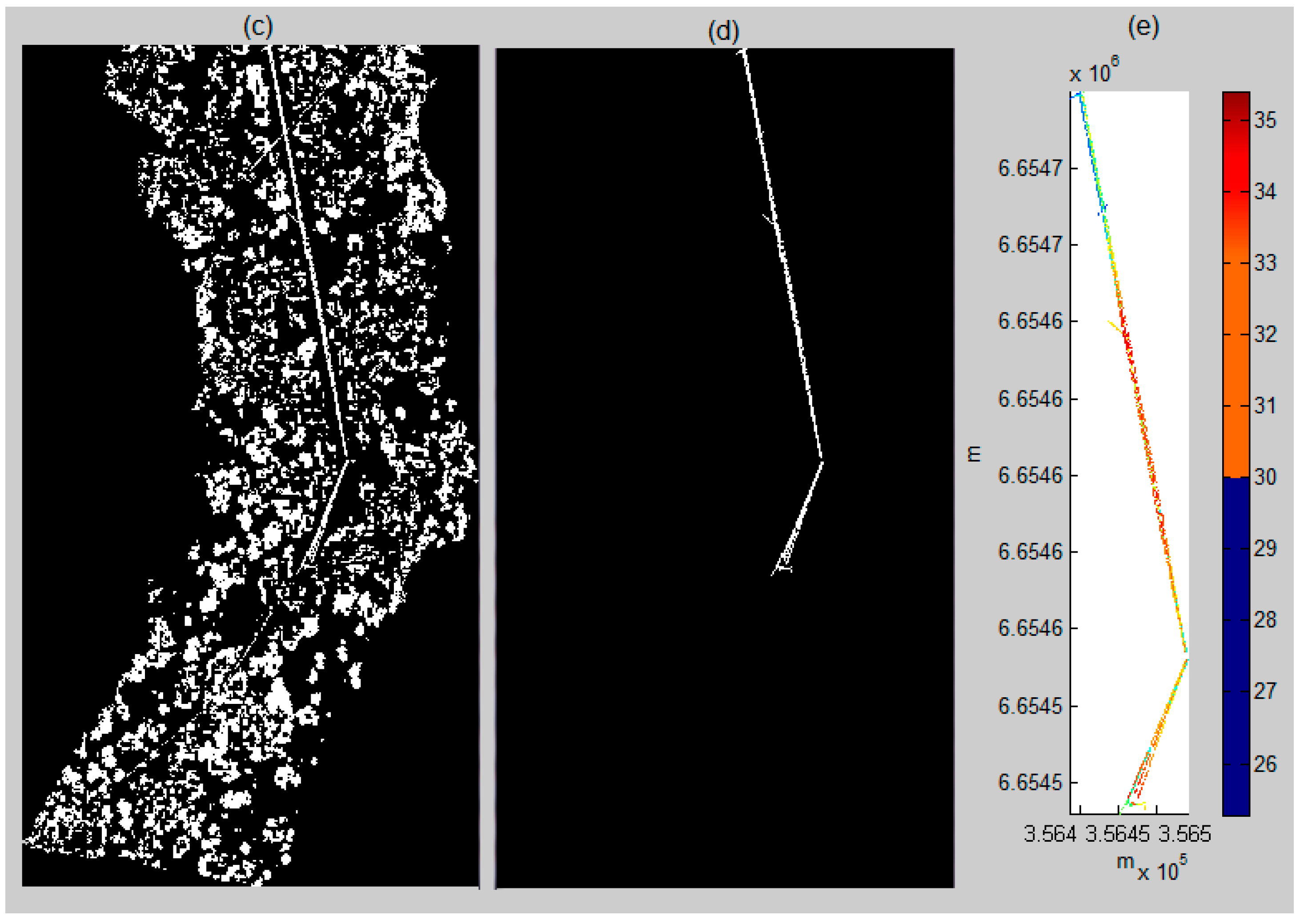
The entire process from the original ALS data to the power line is illustrated in
Figure 4a–e. The data were one of the six test datasets: Area 4.
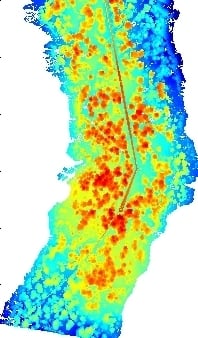
Figure 4a is the original ALS point cloud with a density of 55 points/m
2.
Figure 4b is the power line candidates. It can be observed that after statistical analysis, the power lines became more visible. Moreover, as the number of points was considerably reduced, the subsequent processing became more efficient.
Figure 4c is a binary image that was transferred from
Figure 4b. After the image was filtered by the area size, length and shape, the result yielded
Figure 4d: a power line image. This 2D power line image was transferred to 3D power lines (see
Figure 4e) using the same parameters as in
Figure 4b to
Figure 4c.
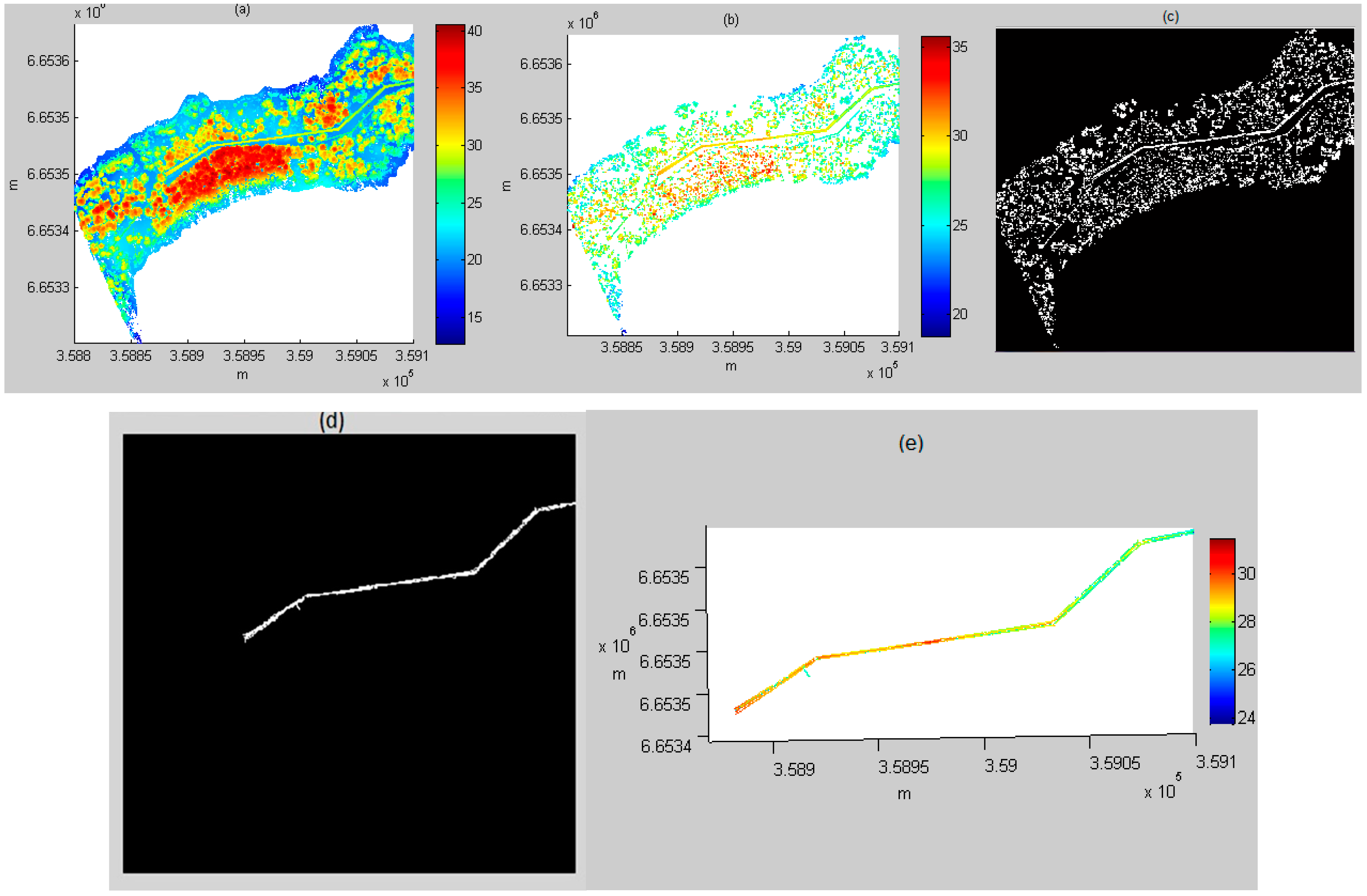
Figure 5 shows another example of the power line extraction in Area 5. It can be observed that the shape of the power lines is different from that in
Figure 4. By applying image processing technology, the power lines were distinguished from their surroundings. This figure also illustrates the entire process. The explanation is the same as that presented for
Figure 4.
Figure 4.
The complete power line process in Area 4. (a) Airborne laser scanning (ALS) point cloud (3D); (b) power line candidate selection (3D); (c) binary image of (b) (2D); (d) after binary image filtering: power line image (2D); (e) extracted power lines (3D).
Figure 4.
The complete power line process in Area 4. (a) Airborne laser scanning (ALS) point cloud (3D); (b) power line candidate selection (3D); (c) binary image of (b) (2D); (d) after binary image filtering: power line image (2D); (e) extracted power lines (3D).
Figure 5.
Power line extraction in Area 5. (a) ALS point cloud (3D); (b) power line candidates (3D); (c) binary image of (b) (2D); (d) after binary image filtering: power line image (2D); (e) extracted power lines (3D).
Figure 5.
Power line extraction in Area 5. (a) ALS point cloud (3D); (b) power line candidates (3D); (c) binary image of (b) (2D); (d) after binary image filtering: power line image (2D); (e) extracted power lines (3D).
3. Results and Discussions
The above-depicted method was conducted with six ALS datasets covering different areas of forests in Kirkkonummi, Finland (
Figure 2). The lengths of the detected power lines in each area are different and vary between 166.13 m and 464.03 m. The total length of power lines is 1.7672 km. The results of power line detection are shown in
Figure 4,
Figure 5,
Figure 6,
Figure 7,
Figure 8 and
Figure 9. The reference data were acquired manually and interactively using Terrascan software (Terrasolid, Finland) and included six sets of power line point clouds. The results were evaluated by statistically evaluating the commission error and omission error, as well as the correctness of the classification. In the classification, the commission error refers to the points classified as a wrong “class”, and the omission error indicates a failed classification.
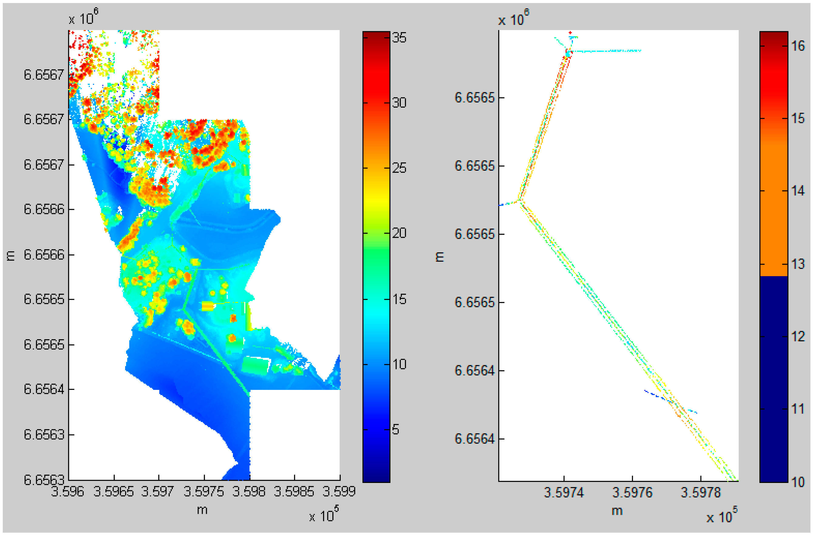
Figure 6,
Figure 7,
Figure 8 and
Figure 9 present the detection results for power lines using the ALS data from Areas 1, 2, 3 and 6, respectively. The results for Areas 4 and 5 are shown in
Figure 4 and
Figure 5. The complete power lines in the six test areas were extracted, and the desired results were achieved.
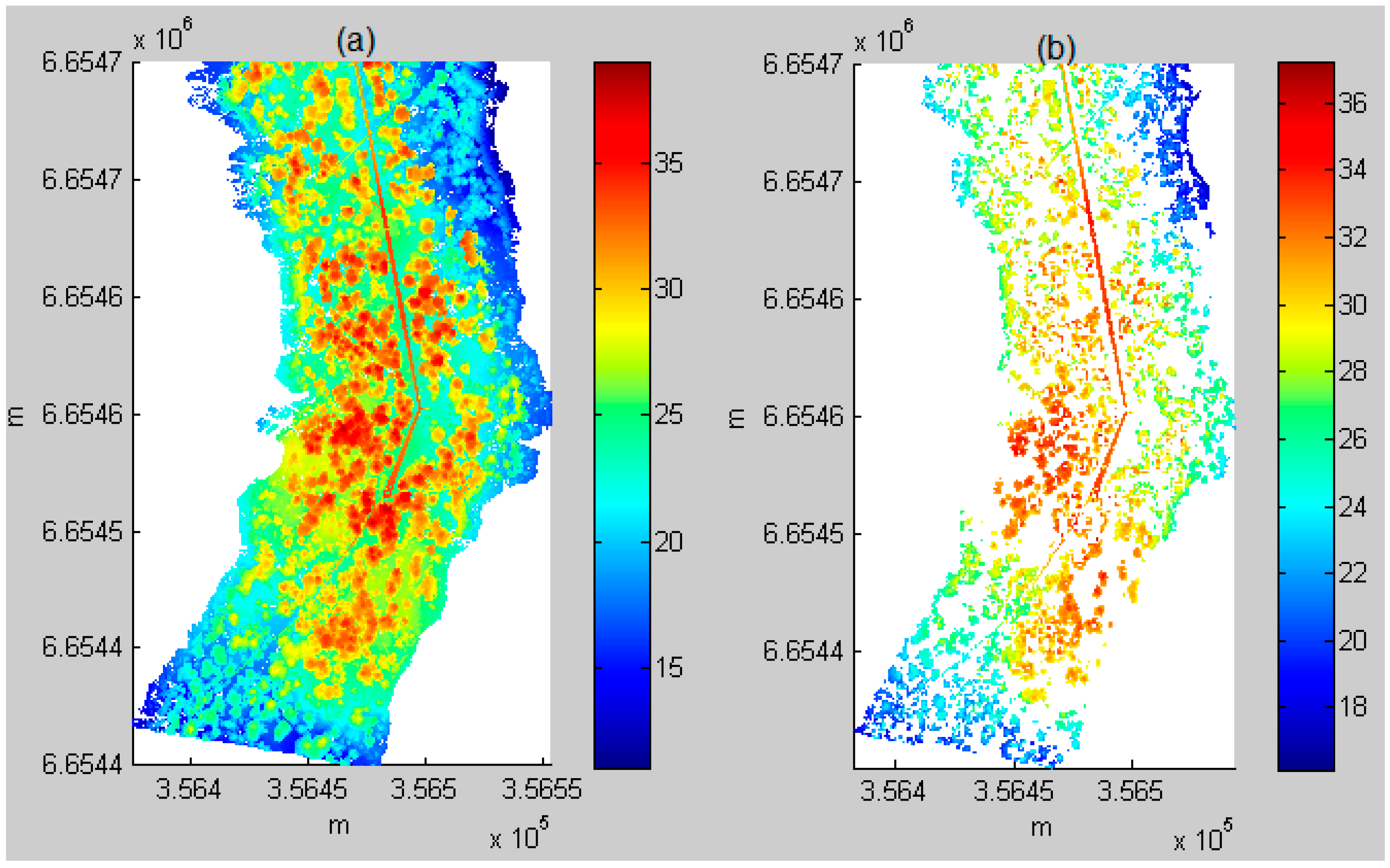
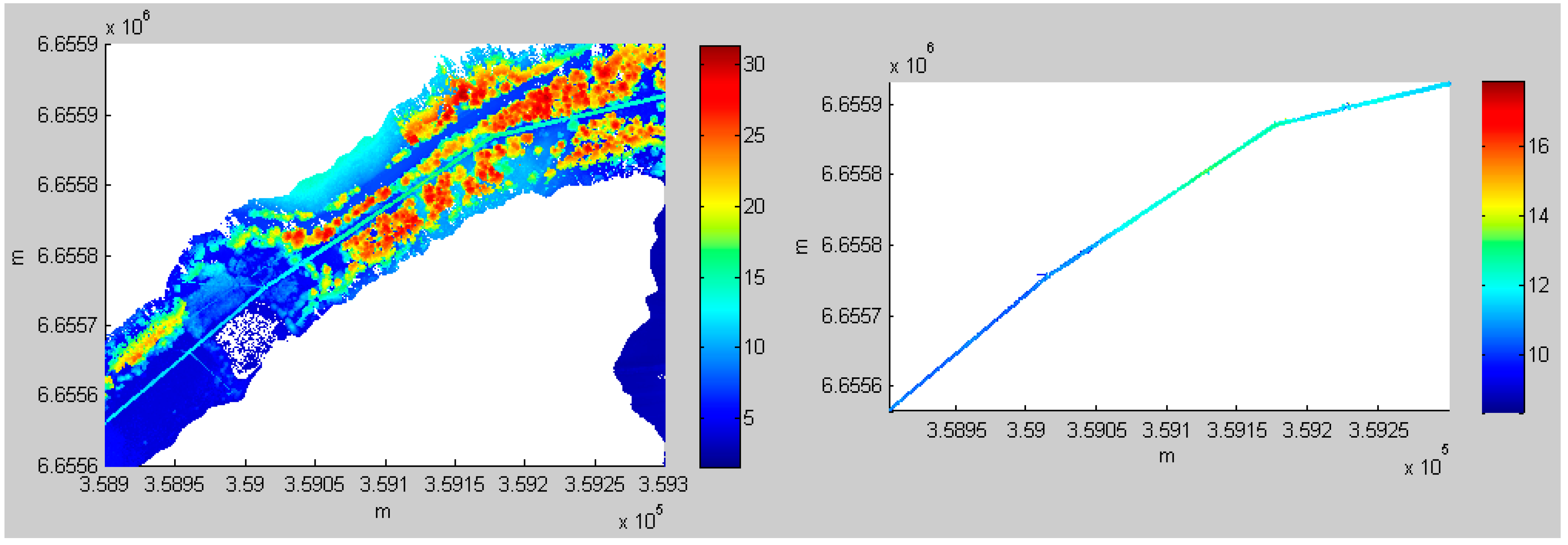
Figure 6.
Power line extraction in Area 1. (Left) ALS point cloud; (Right) the result of power line extraction.
Figure 6.
Power line extraction in Area 1. (Left) ALS point cloud; (Right) the result of power line extraction.
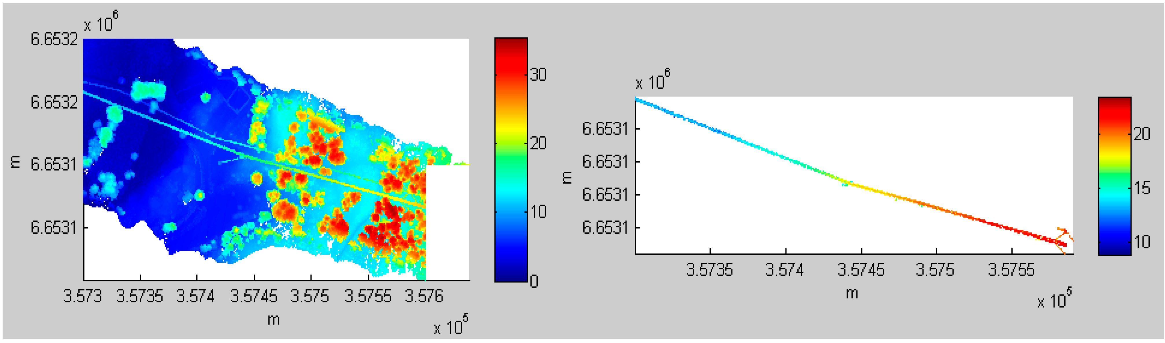
Figure 7.
Power line extraction in Area 2. (Left) ALS point cloud; (Right) the result of power line extraction.
Figure 7.
Power line extraction in Area 2. (Left) ALS point cloud; (Right) the result of power line extraction.
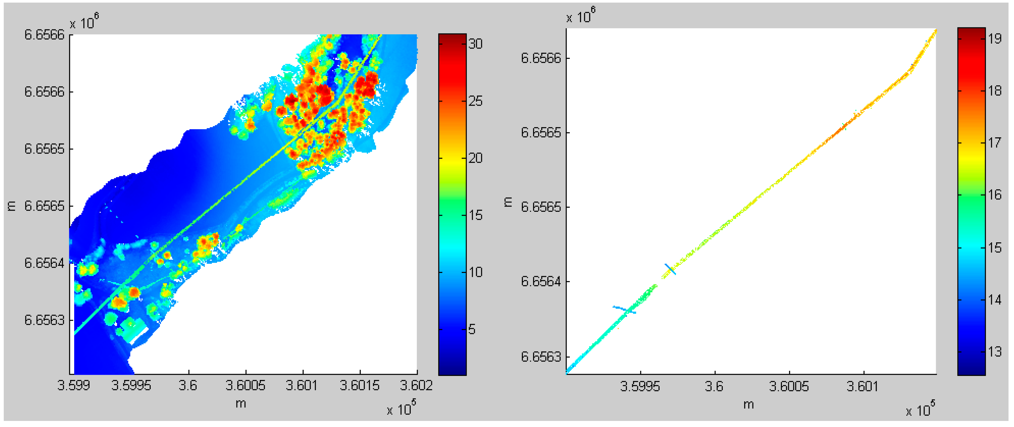
Figure 8.
Power line extraction in Area 3. (Left) ALS point cloud; (Right) the result of power line extraction.
Figure 8.
Power line extraction in Area 3. (Left) ALS point cloud; (Right) the result of power line extraction.
Figure 9.
Power line extraction in Area 6. (Left) ALS point cloud; (Right) the result of power line extraction.
Figure 9.
Power line extraction in Area 6. (Left) ALS point cloud; (Right) the result of power line extraction.
The parameter settings and quantitative results for the test datasets are presented in
Table 3. The parameters include sizeP, Pdensity, paraArea_min, paraArea_max, paraLength and paraShape. The descriptions of the parameters can be found in
Table 1. The parameter values vary according to the different power line shapes, the continuities of the power lines and the closeness between the power lines and trees. For example, the image pixel size is usually determined by the noise level around the power lines. When trees are very close to the power lines, a small pixel size should be applied. However, due to a consistent point density in the test datasets, the parameter “Pdensity” was set to the same value for all datasets. In a binary image, each separated region is called a region. The area of a region can be counted as the number of pixels. When the pixel size of an image is small, e.g., sizeP = 0.5, the area of the region is 20 (pixels); whereas when sizeP = 1, the area of the region is 10 (pixels). Therefore, we say paraArea_min and paraArea_max are not independent. This depends on the pixel size of the image. When “sizeP” changes, not only “paraArea_min” and “paraArea_max”, but also “paraLength” must also be adjusted. “paraShape” determines the shape of the objects that are to be detected. When power lines are line-like, “paraShape” is close to one. For example,
Figure 9 shows power lines that are nearly straight lines (paraShape = 0.99), while
Figure 5 shows power lines that change direction (paraShape = 0.93).
Table 3.
Results for six sets of ALS point clouds.
Table 3.
Results for six sets of ALS point clouds.
| Area ID | Parameters | Number of Points of ALS (point) | Length of Power Lines (m) | Detected Number of Power Lines (point) | Run Time (s) |
|---|
| 1 | Pdensity =
paraArea_min = 100
paraArea_max =1000
paraLength = 70
paraShape = 0.96
sizeP = 0.6 | 3,130,155 | 166.13 | 2348 | 530.47 |
| 2 | Pdensity =
paraArea_min = 80
paraArea_max = 1000
paraLength = 35
paraShape = 0.96
sizeP = 0.60 | 2,874,851 | 269.45 | 3409 | 309.45 |
| 3 | Pdensity =
paraArea_min = 100
paraArea_max = 1000
paraLength = 100
paraShape = 0.92
sizeP = 0.70 | 3,602,719 | 464.03 | 6790 | 530.50 |
| 4 | Pdensity =
paraArea_min = 100
paraArea_max = 1000
paraLength = 70
paraShape = 0.9
sizeP = 0.60 | 3,130,116 | 188.76 | 3295 | 523.09 |
| 5 | Pdensity =
paraArea_min = 100
paraArea_max = 1000
paraLength = 100
paraShape = 0.93
sizeP = 0.60 | 4,781,564 | 380.29 | 7157 | 606.19 |
| 6 | Pdensity =
paraArea_min = 70
paraArea_max = 1000
paraLength = 60
paraShape = 0.99
sizeP = 0.70 | 2,197,719 | 298.50 | 3028 | 167.20 |
The quantitative results in
Table 3 include the number of ALS points, the length of the detected power lines, the number of detected power lines and the run time.
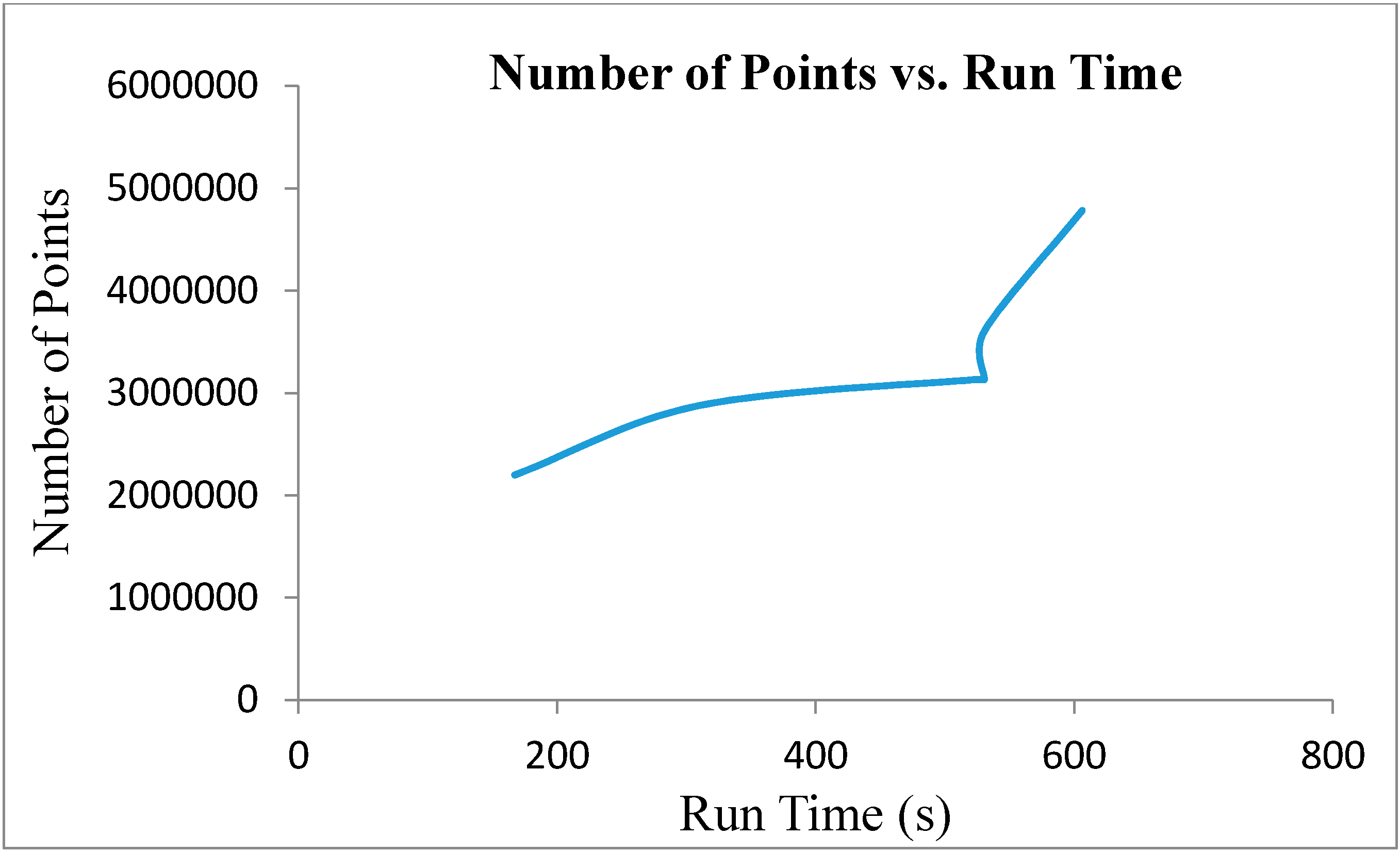
Figure 10 displays the relationship between the number of original ALS points and the run time. It turns out that the run time of the algorithm is proportional to the input number of points.
Table 3 reveals that there is no such relationship between the lengths of the detected power lines or the number of detected power line points and the run time. For example, in Area 1, the length of the power line is 166.1316 m, and the corresponding run time is 530.47 s; while in Area 2, the length of the power line is 269.45 m and the corresponding run time is 309.45 s. Similarly, in Area 1, the number of detected power line points is 2660, and the corresponding run time is 530.47 s; while in Area 2, the number of detected power line points is 6762 and the corresponding run time is 309.45 s.
Figure 10.
The relationship between the number of points in the ALS data and the run time.
Figure 10.
The relationship between the number of points in the ALS data and the run time.
The resultant power line points were visually compared to reference data.
Table 4 presents the statistical evaluation of the results from the six test fields. “Test outcome” is the classification result. Commission error is caused by misclassification, for example if a point belongs to Class “A”, but is misclassified as Class “B”. Omission error refers to a classification failure. The following equations demonstrate the relationship among “Test outcome”, “Reference data”, “Commission”, “Omission” and “True points”.
Table 4.
Evaluation of the results.
Table 4.
Evaluation of the results.
| Area ID | Test Outcome (points) | Reference Data (points) | Commission (points) | Omission (points) | True Points (points) |
|---|
| 1 | 2348 | 2249 | 173 | 74 | 2175 |
| 2 | 3409 | 3256 | 216 | 63 | 3193 |
| 3 | 6790 | 6377 | 509 | 96 | 6281 |
| 4 | 3295 | 3183 | 175 | 63 | 3120 |
| 5 | 7157 | 6681 | 585 | 109 | 6572 |
| 6 | 3028 | 2901 | 175 | 48 | 2853 |
| Total | 26,027 | 24,647 | 1833 | 453 | 24,194 |
Table 5 more intuitively illustrates the results of the evaluation, expressed as percentages. “Correctness”, “Commission error” and “Omission error” can be calculated by the following equations:
Table 5.
Evaluation of the results expressed as percentages.
Table 5.
Evaluation of the results expressed as percentages.
| Area ID | Commission Error (%) | Omission Error (%) | Correctness (%) |
|---|
| 1 | 7.37 | 3.29 | 92.63 |
| 2 | 6.34 | 1.93 | 93.66 |
| 3 | 7.50 | 1.51 | 92.50 |
| 4 | 5.31 | 1.98 | 94.69 |
| 5 | 8.17 | 1.63 | 91.83 |
| 6 | 5.78 | 1.65 | 94.22 |
| Average | 6.74 | 2.00 | 93.26 |
The above evaluation reveals that the correctness for different test fields varies from 91.83% to 94.69%. An average correctness of 93.26% was achieved. The sources of commission error are mainly from small objects or trees that are attached or very close to the power lines. In this case, some noise points were not able to be completely removed. Omission error was mainly caused during candidate selection. When the density criteria and histogram analysis were performed, some threshold values affected the candidate selection. However, the 93.26% accuracy in the forest environment is a promising result. This finding is comparable with the latest results from the non-forest area, such as those reported by Cheng
et al. (2014) [
21] (93.9%) and by Kim and Sohn (2013) [
5] (93.8%).
In the future, we will use combined methods to improve the accuracy and separation between lines and curvature calculations will be developed.
4. Conclusions
This paper presented an automated, computationally-effective power line detection method for lower voltage power lines surrounded by forests. We utilized a statistical analysis method and image-based processing technology for power line classification. During the stage of statistical analysis, a set of criteria (e.g., height criteria, density criteria and histogram thresholds) is applied for selecting the candidates of power lines. After transforming the candidates into a binary image, image-based processing technology is employed. Object geometric properties are considered as criteria for power line extraction. Our method was conducted with six sets of ALS point clouds with an average point density of 55 points per m2. By applying our algorithms, the power lines were detected with an average accuracy of 93.26%. These findings are comparable with the latest results for non-forest areas. The advantages of our method are as follows:
(i) The completeness of power lines: power lines were extracted as whole objects instead of connecting pieces of the lines;
(ii) Despite the forest environment, the accuracy of the classification is still comparable to that of classification in non-forest environments;
(iii) Our method can be applied to power lines with multiple directional turning points;
(iv) This method can also be used for urban areas and open zones. It is beneficial from the adjustability of the parameters. In the case of urban or open environments, better results can be achieved.
Due to the scarce research reported for forest environments, our work may inspire more researchers to work in this field and achieve better results.


