Article

Estimation of Daily Air Temperature Based on MODIS Land Surface Temperature Products over the Corn Belt in the US

1
State Key Laboratory of Information Engineering in Surveying, Mapping and Remote Sensing, Wuhan University, Luoyu Road No. 129, Wuhan 430079, China
2
Center for Advanced Land Management Information Technologies, University of Nebraska-Lincoln, 3310 Holdrege St, Lincoln, NE 68583, USA
3
National Drought Mitigation Center, University of Nebraska-Lincoln, 3310 Holdrege St, Lincoln, NE 68583, USA
4
School of Civil Engineering, Purdue University, 550 Stadium Mall Drive, West Lafayette, IN 47907, USA
5
Collaborative Innovation Center for Geospatial Technology, Luoyu Road No. 129, Wuhan 430079, China
6
Changjiang River Scientific Research Institute, Changjiang River Water Resources Commission, Huangpu Street No. 23, Wuhan 430010, China
*
Author to whom correspondence should be addressed.
Remote Sens. 2015, 7(1), 951-970; https://0-doi-org.brum.beds.ac.uk/10.3390/rs70100951
Submission received: 7 October 2014 / Accepted: 5 January 2015 / Published: 15 January 2015

Abstract

:
Air temperature (Ta) is a key input in a wide range of agroclimatic applications. Moderate Resolution Imaging Spectroradiometer (MODIS) Ts (Land Surface Temperature (LST)) products are widely used to estimate daily Ta. However, only daytime LST (Ts-day) or nighttime LST (Ts-night) data have been used to estimate Tmax/Tmin (daily maximum or minimum air temperature), respectively. The relationship between Tmax and Ts-night, and the one between Tmin and Ts-day has not been studied. In this study, both the ability of Ts-night data to estimate Tmax and the ability of Ts-day data to estimate Tmin were tested and studied in the Corn Belt during the growing season (May–September) from 2008 to 2012, using MODIS daily LST products from both Terra and Aqua. The results show that using Ts-night for estimating Tmax could result in a higher accuracy than using Ts-day for a similar estimate. Combining Ts-day and Ts-night, the estimation of Tmax was improved by 0.19–1.85, 0.37–1.12 and 0.26–0.93 °C for crops, deciduous forest and developed areas, respectively, when compared with using only Ts-day or Ts-night data. The main factors influencing the Ta estimation errors spatially and temporally were analyzed and discussed, such as satellite overpassing time, air masses, irrigation, etc.

1. Introduction

Air temperature (Ta) plays an important role in energy balance and is a key input in various environmental models and applications, such as crop evapotranspiration estimation [1], distributed hydrology [2] and climate change models [3]. Ta is typically measured at meteorological stations 2 m above the ground. Meteorological measurements provide accurate discrete Ta information for specific locations but have limited ability to describe its spatial heterogeneity over large areas [4,5]. The non-uniform spatial distribution of weather station locations within most networks and the complexity of the land surface conditions and patterns make it a challenge to get spatial-continuous Ta data.
Satellite remote sensing observations from global imaging sensors, such as the Advanced Very High Resolution Radiometer (AVHRR) and Moderate Resolution Imaging Spectroradiometer (MODIS), represent a potentially valuable alternative to characterize spatially-detailed Ta patterns across large areas. A split window technique was applied to AVHRR [6], MODIS [7], and Meteosat [8] thermal data to estimate Land Surface Temperature (LST). The science-grade quality of the LST data collected by MODIS has proven valuable for monitoring land surface dynamics over large areas [4,9,10].
The earth’s surface is heated by solar radiation, while the atmosphere is mainly heated from the ground up through longwave infrared radiation [11]. The relationship between Ts (Land Surface Temperature) and Ta may vary with time and location, because the land surface energy balance is a complex phenomenon that depends on multiple factors (e.g., cloud cover, surface roughness, wind speed and soil moisture), whereas some of them (e.g., wind speed) are usually not available from satellite [12,13,14]. Zakšek and Schroedter-Homscheidt [15] and Benali et al. [4] reviewed the types of methods commonly used to estimate Ta from satellite-based LST products. These can be divided into three distinct types of approaches.
The first type are statistical approaches based on a simple linear regression between Ts and Ta, or advanced statistical models with consideration of more than one independent variable, such as solar zenith angle (SZA), elevation, altitude, Julian day among others [10,16,17]. Lin et al. [10] used stepwise linear regression method to estimate daily maximum air temperature (Tmax) and daily minimum air temperature (Tmin) with MAE = 1.9, agreement index = 0.79 and MAE = 1.9 °C, agreement index = 0.92, respectively, over east Africa. Fu et al. [18] used linear regression between MODIS Ts and Tmax from stations on the northern Tibetan Plateau. In general, these methods perform well within the spatial and time frame they were developed, but the accuracy might decrease when extended in time and space [14].
The second category is index-based methods such as the Temperature-Vegetation index (TVX). It is a contextual method based on the hypothesis that for thick vegetation canopy temperature approximates Ta [19,20]. The negative relationship between the Normalized Difference Vegetation Index (NDVI), which serves as a general indicator of vegetation greenness, and Ts in the study area is the foundation for the application of this method. Zhu et al. [21] used the TVX method to estimate daily Tmax with RMSE (the root mean square error) =3.709 °C, MAE (the mean absolute error) = 3.03 °C and r (correlation coefficient) =0.83 in Xiangride River Basin of China. However, Vancutsem et al. [22] found that TVX method did not adapt to different ecosystems over Africa because non-significant relationship between Ts and NDVI in their study. Karnieli et al. [23] found that the approaches based on this negative NDVI/Ts relationship have minimal utility in energy-limited environments (e.g., high latitude and elevations) compared to moisture-limited environments because vegetation-expressed NDVI response is more related to available solar radiation than land surface conditions (e.g., soil moisture).
The final class of methods uses surface energy balance parameterizations based on physically-based models [24]. The sum of incoming net radiation is considered equal to the sum of the soil heat flux, sensible flux and latent heat flux [15,24]. However these methods require large amounts of information that are usually not only from remote sensing (e.g., roughness, soil physical properties) [4,9,13].
Benali et al. [4] used both weekly daytime LST data (Ts-day) and nighttime LST data (Ts-night) to estimate the average, maximum and minimum weekly temperature. They found that there was a higher correlation between average weekly temperature and averaged weekly Ts-night, which indicates the potential of Ts-night in estimating averaged weekly temperature. However the relationships between daily Tmax and Ts-night have not been investigated in previous studies.
The main objective of this study was to estimate daily Tmax (hereafter Tmax) and daily Tmin (hereafter Tmin) across the U.S. Corn Belt region based on both Ts-day and Ts-night observations acquired from MODIS and auxiliary variables. Previous studies aimed at estimating Tmax have been based on Ts-day data only and generally applied to small areas and/or a small number of meteorological stations [14,16,25,26]. In this study, the work was extended to include Ts-night data and applied for a five-year period (2008–2012) over the U.S. Corn Belt, which represents a large, agriculturally-significant region that covers six states. Ta plays an important role in understanding regional variations in crop phenology via growing degree days (GDD) [27] and environmental stress, such as drought, which are important in assessing potential crop production. The ability to monitor Ta over this area has enormous economic and strategic significance given its role as a major producer of corn and soybeans. This study analyzed the spatial and temporal relationship between daily Ta and Ts at both the local weather station scale and the regional scale using satellite-derived gridded Ts data sets. The main factors influencing the Ta estimation errors spatially and temporally were also analyzed and discussed.

2. Study Area

The Corn Belt region of the Midwestern United States is considered to be the breadbasket of the country because of extensive corn and soybean production. The study area includes six states (Iowa, Illinois, Indiana, parts of Minnesota, Nebraska, and Ohio) that comprise 52 Agricultural Statistics Districts (ASDs) (Figure 1). There are geographic variations in temperature, precipitation, elevation across this sizable study area. The elevation is increasing from east-to-west with elevations ranging from 87 to 666 m. Precipitation increases in a west-to-east direction ranging from the lowest annual precipitation of about 500 mm in Nebraska to about 1300 mm in eastern locations. Temperature generally decreases with latitude across the study area with subtle local-scale variations because of topographic elevation differences. Corn and soybeans are the major crops planted across the Corn Belt with most of the U.S. top production states (Illinois, Iowa, Nebraska, Minnesota) being located within this region [28]. Usually, they were planted in May or before and harvested in September or later. Accordingly, the period from May to September was included as the growing season in this study. The majority of the Corn Belt produces corn and soybeans under rainfed conditions because in normal climatic years most of the region receives ample precipitation to sustain high crop production levels. The exception is the state of Nebraska, where irrigated systems have been implemented because of lower annual rainfall rates.
Figure 1. Map of the U.S. Corn Belt study area with the main land-cover types (from Cropland data layer data (CDL) of 2012) and spatial distribution of the meteorological stations used in this study presented.
Remotesensing 07 00951 g001

3. Data Description and Processing

3.1. MODIS Data

Daily 1000 m LST data (MOD11A1 and MYD11A1, Collection 5, from MODIS sensors on board Terra and Aqua satellites, respectively) for the period of 2008–2012 during the growing season (May to September) over the Corn Belt were used. The study area covers four MODIS tiles (i.e., h10v04, h10v05, h11v04, and h11v05). The data were downloaded from NASA’s Earth Observing System Data and Information System [29]. The nominal equatorial passing time of Terra is around 10:30 a.m. and 10:30 p.m. local solar time, while Aqua passes in the opposite direction at about 1:30 a.m. and 1:30 p.m. As a result, the Aqua and Terra MODIS instruments collectively provide four daily LST observations, which enabled analysis of those four selected times and day, night, and day/night LST differences in this study. A 13 by 13 pixel window centered by the station was used to get average Ts, as Prihodko and Goward (1997) [19] stated that Ta deviations of approximately 0.6 °C occur at horizontal distances of 6 km.

3.2. Weather Station Data

Daily Tmax and Tmin measured in weather stations from 2008 to 2012 were downloaded from the GHCN (Global Historical Climatology Network) daily database from NOAA’s National Climatic Data Center [30]. This database is a composite of climate records from numerous data sources that were merged and then checked for quality assurance. For analysis, the stations were divided into three sub-datasets according to the dominant land cover surrounding each station location: crops (corn and soybeans), developed areas and deciduous forest. These three classes were selected because they represent the primary land-cover types in the study area.

3.3. Auxiliary Data

Additional auxiliary data were used to refine the analysis that included: The NASS Cropland Data Layers [31]; irrigation data from the MODIS Irrigated Agriculture Dataset (MIrAD) [32]; elevation; Julian day; and SZA. The NASS CDLs from 2008 to 2012 for the Corn Belt states were used to select crops, deciduous forest and developed area pixels around the stations. The weather stations were selected by three steps based on CDL data. Firstly, the original 30-m CDL data were resampled to 25-m spatial resolution by nearest neighbor resampling. Then the 25-m spatial resolution CDL data was resampled to 1-km spatial resolution to be consistent with the MODIS LST datasets by calculating the 25-m spatial resolution pixels of each land-cover types within the 1-km by 1-km pixel window. The 1-km pixel was marked as one of the three targeted land-cover types when the 1 km by 1 km pixel window was covered by more than 75% of 25-m pixels of such land cover type, or it was marked as other types. Finally, station locations were considered to be surrounded by a dominant land cover type when one of the three targeted land cover classes comprised more than 50% of the 1-km pixels within a 13-by-13 pixel window centered on each station. Only station locations with a dominate land cover type were retained for analysis and Ts values in the MODIS LST were extracted from only the pixels of the dominant land cover type to calculate the Ts of the station location. Solar zenith angle was calculated based on both latitude and Julian day [33].

3.4. Data Processing

It is important to eliminate low quality data in the MODIS LST data because remote sensing based Ta estimates are strongly influenced by errors (e.g., error caused by cloud cover and large sensor viewing angles, uncertainties in surface emissivity [34]) of the LST retrievals [4]. Validation studies of MODIS Ts show that under clear-sky conditions the precision is approximately 1 K or less, but higher errors would be observed at large viewing angles and in semiarid regions [35]. So only the pixels of the targeted land-cover types that were flagged in the MODIS quality assurance data as cloud-free and of high quality were retained. However, there is still undetected cloud-contaminated LST outliers occurring at cloud edges and these typically have negative °C temperature values [36]. In order to minimize these cloud-contaminated pixels, only Ts value of the station which has larger than 90% cloud-free pixels in the 13-by-13 window were selected [14]. In addition, pixels were eliminated if they were outside the 0–120 °C and 11–130 °C sensor zenith angle ranges, for day and night products, respectively [4].

4. Methodology

Model design and assessment was based on linear regression analysis. Other factors, such as the Julian day, solar zenith angle, latitude, and elevation, which may affect the Ts-Ta relations as described in previous papers [10,16,17], were also taken into consideration. The refined dataset was divided into two groups: calibration and validation datasets with a 70%/30% split into these groups using a simple random sampling. It is an efficient way to obtain unbiased results.
The statistical relationship between MODIS Ts products and station-based daily Ta was analyzed in this study. Four statistical performance measures were used including the common correlation coefficient (R), the mean bias (the difference between the estimated and observed values), MAE, and RMSE. The RMSE is particularly sensitive to outliers on an individual level [37]. Collectively, these performance statistics were analyzed to characterize model performance and the impact of seasonality and spatial location on estimation accuracy of Ta from MODIS Ts data.
In addition, ground-air temperature difference (GATD) and diurnal temperature range of Ts (Ts-DTR), which were defined as Equations (1) and (2), respectively, were introduced to analyze Tmax estimation. GATD is usually referred to the difference of Ts and Ta value of the same time. However, in this study, the time when Ts-day was acquired and the time when Tmax reached were not exactly the same (about 0~3 h difference). We assume that the difference of the acquired time of Ts-day and Tmax had little impact on GATD.
GATD=Tsday  Tmax
Ts-DTR=Ts-day Ts-night
Inter-diurnal variability (IDV) of Ta was introduced to analyze the spatial and temporal patterns of Ta estimation accuracy. It refers to the day-to-day changes of Ta (Tmax/Tmin) in a given meteorological element [38]. It can be taken as the numerical difference between successive daily extremes (Tmax/Tmin) [38] (Equation (3)). When IDV is averaged over the entire study period (e.g., for a particular month), the resulting quantity is referred to as the mean inter-diurnal variability of temperature (MIDV) [39] (Equation (4)):
IDVt=TatTat1
MIDV= Start End (TatTat1) N
where ID V t refers to the IDV of the t day (t = 1, 2, 3, …). T a t and T a t1 refers to the Ta (Tmax/Tmin) of the t day and t − 1 day (the day before the t day). Start and End are the first and last day of the study period for MIDV, respectively. N is the number of days during the study period for MIDV.

5. Results and Discussion

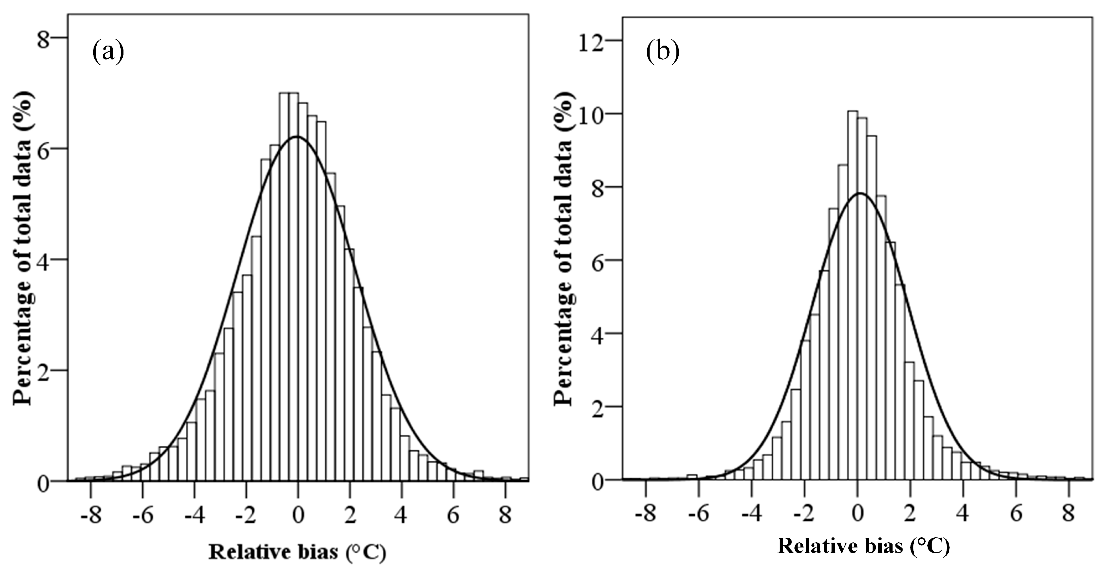
5.1. The Relationship between Observed Ta and Ts from MODIS Terra and Aqua

The influence of the time-of-observation on estimation of Ta has been studied and discussed in several previous studies that resulted different conclusions. For example, Benali et al. [4] stated that the use of both Aqua Ts-day and Ts-night could improve the estimation of Tmax and Tmin, respectively, due to the fact that the MODIS Aqua overpass time is closer to the time of both Tmax and Tmin than Terra’s. In contrast, Zhu et al. [21] showed that both Terra Ts-day and Ts-night were better than Aqua Ts-day and Ts-night for Ta estimations in Xiangride River basin of China. In another study, Mostovoy et al. [9] found that the difference between satellite overpass (Terra and Aqua) had little impact on the estimation accuracy of Ta.
The comparison between MODIS Ts data and Ta observations shows that Ts-day from both Terra and Aqua, with the mean relative bias above zero, tended to overestimate Tmax (Table 1). The Ts value of daytime Aqua LST is higher than that of daytime Terra LST, which might be expected given the fact that more solar radiation has been received at the time of the Aqua MODIS overpass later in the day. As a result, a higher relative bias was observed for the Aqua Ts-day than Terra Ts-day, though the time when Aqua Ts-day was acquired was closer to the time when Tmax was reached. Both Aqua Ts-night and Terra Ts-night overestimated Tmin as well. As both minimum Ts and Ta usually occur near or after sunrise [40]. The nighttime overpasses of MODIS occurs before the both minimum Ts and Ta is reached, which led to this observed higher Ts values from both MODIS sensors relative to the observed Tmin. This is supported by the fact that the Ts from Terra MODIS, which has an overpass time ~3 h before the MODIS Aqua overpass, consistently had higher Ts values reflecting the cooling of the land’s surface as the night progresses. Compared to the value of Terra Ts-night, that of Aqua Ts-night was closer to Tmin value.
Table 1. Statistics with direct using of daily MODIS Ts products as estimators of Ta observations (°C).
DatasetsMeanbiasRMSEMAER
MODday & Tmax1.394.963.660.46
MODnight & Tmin2.263.062.540.93
MYDday & Tmax3.826.394.740.46
MYDnight & Tmin0.512.041.480.95
MODday: MOD11A1 Ts-day from Terra; MODnight: MOD11A1 Ts-night from Terra; MYDday: MYD11A1 Ts-day from Aqua; MYDnight: MYD11A1 Ts-night from Aqua.

5.2. Ta Estimation from MODIS Ts

Several models using the variables in Table 2 to estimate Ta from the MODIS Ts observations by multiple linear regression were developed and tested. Having similar results for the calibration and validation samples, means that the Ts and Ta relationships were consistent throughout the dataset, i.e., independently of the subset. Similar to previous studies, better performance of Tmin estimation than Tmax estimation was observed. For Tmax, the models with only Ts-night have significantly higher accuracy than the models with only Ts-day. This was consistent across all three land-cover types with the most notable result over crop areas, which had a decrease in RMSE and MAE by 1.66 °C and 1.29 °C for Terra Ts and 1.53 °C and 1.23 °C for Aqua Ts, respectively (Table 2, Models 1–4). The combination of both Ts-day and Ts-night improved the estimation accuracy for both Terra and Aqua (Table 2, Models 5 and 6). There were smaller differences between Terra-day and Aqua-day, however Terra-night was a better explanatory variable of Tmax than Aqua-night (Table 2, Models 1–6). When Julian day and SZA were used as a seasonal correction effect in Tmax estimation, model performance increased slightly when compared with using only Ts variables in all three land-cover types. When latitude and elevation were considered, the accuracy of models was relatively unchanged.
Table 2. Model variables and validation accuracy for Tmax and Tmin (°C).
Model (Tmax) CropsForestDevelopedModel (Tmin) CropsForestDeveloped
(1) MODdayRMSE4.243.323.32(11) MODdayRMSE5.084.434.06
MAE3.292.612.55MAE4.023.513.27
R20.210.610.53R20.120.440.42
(2) MODnightRMSE2.582.572.65(12) MODnightRMSE1.972.032.06
MAE2.002.042.04MAE1.511.581.58
R20.710.770.69R20.860.880.85
(3) MYDdayRMSE4.273.403.56(13) MYDdayRMSE5.134.484.12
MAE3.352.662.93MAE4.063.543.37
R20.200.590.55R20.100.420.40
(4) MYDnightRMSE2.742.702.69(14) MYDnightRMSE1.841.831.82
MAE2.122.112.10MAE1.361.361.36
R20.670.740.67R20.880.900.88
(5) MODday + MODnightRMSE2.392.202.39(15) MODday + MODnightRMSE1.952.032.04
MAE1.851.771.89MAE1.491.591.59
R20.750.830.74R20.860.880.85
(6) MYDday + MYDnightRMSE2.512.312.34(16) MYDday + MYDnightRMSE1.811.821.81
MAE1.921.841.83MAE1.331.361.35
R20.720.810.76R20.880.900.88
(7) MODday + MODnight + DOYRMSE2.272.172.33(17) MYDnight + DOYRMSE1.761.822.14
MAE1.741.751.86MAE1.301.341.69
R20.770.830.76R20.880.900.88
(8) MODday + MODnight + SZARMSE2.312.192.28(18) MYDnight + SZARMSE1.751.822.36
MAE1.771.751.80MAE1.301.361.91
R20.770.830.77R20.880.900.88
(9) MODday + MODnight + LatRMSE2.392.152.38(19) MYDnight + LatRMSE1.841.821.81
MAE1.851.711.89MAE1.351.351.34
R20.750.830.74R20.880.900.88
(10) MODday + MODnight + ElevRMSE2.312.202.32(20) MYDnight + ElevRMSE1.841.842.00
MAE1.771.761.82MAE1.361.381.49
R20.770.830.76R20.880.900.88
DOY: Day of year (e.g., 1–365); SZA: Solar zenith angle; Lat: Latitude; Elev: Elevation.
For Tmin estimation, models with only Ts-day had the lowest accuracy and when daytime and nighttime LST were combined, no significant improvement in accuracy was found compared to the results with Ts-night only (Table 2, Models 11–16). This indicates that Ts-day is not relevant for Tmin estimation. Aqua Ts-night provided a better estimation of Tmin than Terra Ts-night. The inclusion of Julian day and SZA in both of these models only yielded slight accuracy increase when compared with using only Ts-night over crop and forest areas, while over developed areas, no increase in Ta estimation accuracy was found. Models 7 and 17 including DOY were found to have the highest accuracy in estimating Tmax and Tmin for crop and forest areas, respectively. Thus, these models were selected for further study in crop and forest areas. For developed areas, given the fact that the estimation accuracy of Model 7 was only slightly lower than the highest one (RMSE greater than the one with highest accuracy by 0.05), it was selected for Tmax estimation to be consistent with crop and forest areas for comparison. For Tmin estimation, it is noticed that Model 17 had an obvious lower accuracy compared to Model 14 (RMSE of Model 17 greater than that of Model 14 by 0.32). Moreover, combining other variables (MODday, latitude) only decreased the RMSE by 0.01–0.03. Having cost and complexity of models taken into consideration, Model 14 that included only Aqua Ts-night was used for further analysis for developed areas.
Using the selected models, the frequency distribution of the relative bias between estimated Ta and observed Ta for all three land-cover types is close to the normal distribution curves and almost symmetrical with the mean bias centered in zero (0.01 for Tmax estimation and 0.06 for Tmin estimation). The temperature error ranged between −8 °C and 8 °C (Figure 2). For Tmax, approximately 38%, 66%, and 83% of all estimations were within 1 °C, 2 °C, and 3 °C absolute bias, respectively. For Tmin, approximately 50%, 79%, and 92% of all estimations were within 1 °C, 2 °C, and 3 °C absolute bias, respectively.
Figure 2. Relative bias distribution considering all Tmax (a) and Tmin (b) estimations with the selected models in the study area for all the three land-cover types. (The black curves are the normal distribution curves).
Remotesensing 07 00951 g002
At the regional scale, the estimation accuracy of both Tmax and Tmin varied with phases of the growing season. For all the three land-cover types (i.e., crops, forest, and urban), the accuracy of estimated Tmax and Tmin was higher in June, July, and August) than that either in May or September (Figure 3). Performance was also analyzed for each meteorological station. Results showed that about 83% of the stations had a correlation higher than 0.80, MAE lower than 1.50 °C and RMSEs lower than 2.5 °C for Tmax. By comparison, about 85% of the stations had a correlation higher than 0.88, MAE lower than 1.10 °C and RMSEs lower than 2.0 °C for Tmin. Generally, the stations located in deciduous forest had a better performance than those in crop and developed areas. The spatial distribution of RMSE shows that the majority of the stations with lower performance in Tmax estimation were located in the areas with higher elevation (specifically, east of Nebraska and northwest of Iowa) and in the northeast of Illinois (Figure 4). The spatial and temporal patterns are discussed in Section 6.2.
Figure 3. Accuracy of estimated Tmax (ac) and Tmin (df) (RMSE, °C) in different months from 2008 to 2012 over three land-cover types (forest, developed and crop).
Remotesensing 07 00951 g003
Figure 4. Spatial distribution of Tmax (a) and Tmin (b) (°C) estimation accuracy (RMSE) for all the meteorological stations.
Remotesensing 07 00951 g004

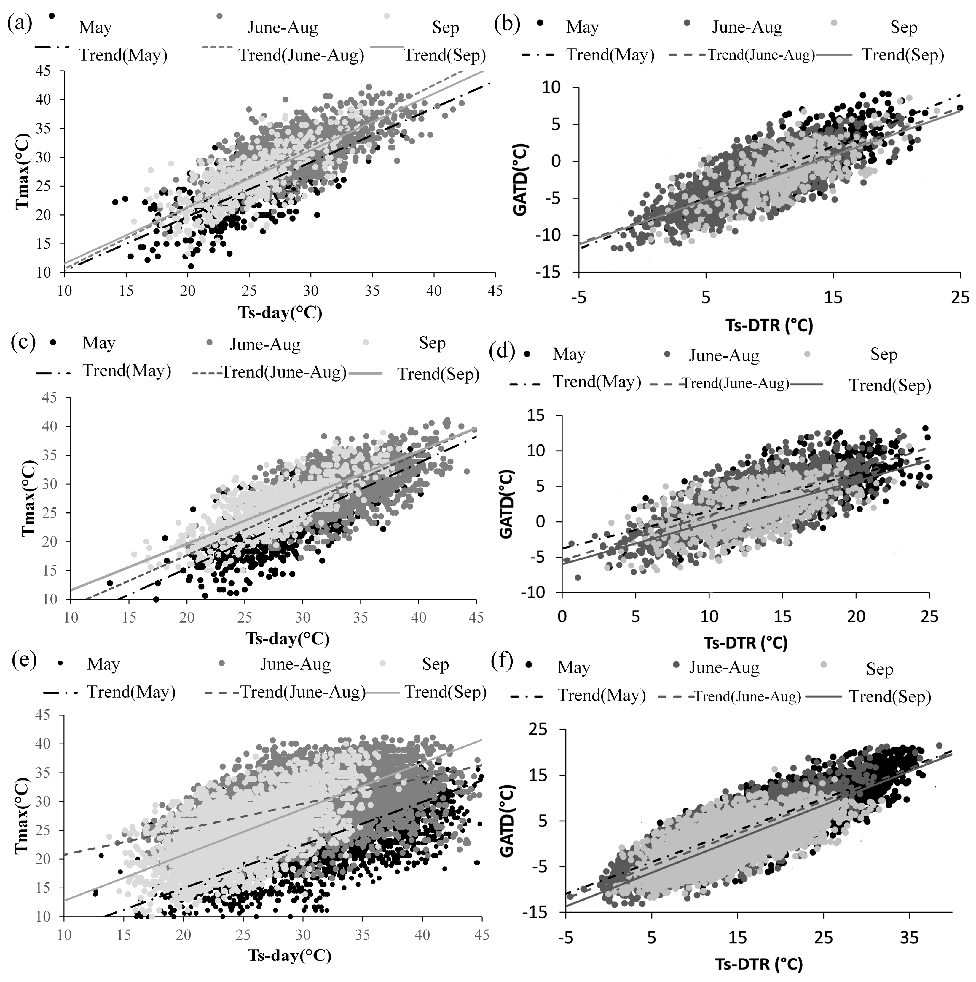
5.3. Correlation Analysis of MODIS Ts and Tmax

It is interesting that Tmax has stronger agreement with Ts-night than Ts-day. In addition, higher Tmax estimation accuracy was observed with the combination of both Ts-day and Ts-night than with either of them alone. As shown in Table 2, Ts-day and Tmax have similar correlation coefficient in deciduous forest and developed area, while it is significantly lower in cropland. Fu et al. [18] also found that estimation using linear regression of Tmax from MODIS Ts-day was not accurate enough in the growing season (p > 0.01, R2 < 0.10) compared to the non-growing season (p < 0.01, R2 > 0.40). In cropland areas, the Ts-day and Tmax relations can be varied and complex at different periods during the growing season, as the vegetation cover is changing over time and different crop types are planted in rotations from year to year. As shown in Figure 5e, compared with Figure 5a,c notable differences can be observed in Tmax and Ts-day relationship during different phases of the growing season in crop areas. While, it is shown from Figure 5b,d,f that both GATD and Ts-DTR have similar linear correlation relationships (trend) in different seasons from May to September for all three land-cover types, especially for crops compared to the relation between Ts-day and Tmax.
Figure 5. Scatterplot of Ts-day vs. Tmax (°C) and GATD vs. Ts-DTR (°C) for: (a,b) forest; (c,d) developed; and (e,f) crops areas across the entire study area from 2008 to 2012.
Remotesensing 07 00951 g005
As at the beginning of the growing season, vegetation fraction is low and the land’s surface is composed primarily of bare soil. Ts-day is usually much higher than Tmax during this period as more energy is partitioned into sensible heat flux from the soil as opposed to later in the year when crops have emerged and are transpiring (latent heat flux) [41]. During the green-up phase of crops, the spatial coverage of vegetation increases, leading to transpirational cooling, increased latent heat fluxes, decreased sensible heat fluxes, and in general a reduced daytime GATD [41]. During the senescence phase of crops, as maturity is reached, photosynthesis and transpiration decrease, the latent heat fluxes decreases, the sensible heat fluxes increase resulting in higher GATD [41]. Thus, over crop areas Ts-day is typically much higher than Tmax at the beginning of the growing season, slightly lower than or equal to Tmax in the middle stage of the growing season and slightly higher than or equal to Tmax in the end of the growing seasons (Figure 6c). While in deciduous forest and developed area, Tmax increases with Ts-day proportionally and the seasonality effect is minimal (Figure 5a,c, Figure 6a,b).
Figure 6. Typical Tmax, Ts-day and Ts-night (°C) curves (ac), Ts-DTR and GATD (°C) curves (df), of three land-cover types: (a,d) deciduous forest (in Albia 3 NNE, 2009); (b,e) developed (in Columbus port Columbus international airport, 2009); and (c,f) crops (in Little Sioux 2 NW, 2009).
Remotesensing 07 00951 g006
As expected, a strong linear relation between GATD and Ts-DTR was observed for all stations from 2008 to 2012 in the study area (Figure 7). It is the reason why combining Ts-day and Ts-night to estimate Tmax could minimize the influence of these factors and a higher accuracy could be achieved. In the absence of solar radiation, Ts-night is affected by fewer factors and is more stable than Ts-day [10,21,22]. Even with the same solar radiation, the relationship between Ts-day and Tmax is affected by several factors like vegetation changes, land-cover types, soil moisture, precipitation, wind speed, etc. [4,20]. Similarly, with the same solar radiation, the relationship between Ts-day and Ts-night is affected by the abovementioned factors in the same way. Many previous studies have shown that both GATD and Ts-DTR increase with elevation and decrease with increased vegetation cover, cloud cover, soil moisture and precipitation, respectively [19,20,25,42,43,44]. For example, in the developed or low soil moisture areas (e.g., desert), both the DTR and Ts-day can be much higher than that of forest areas or wet areas.
Figure 7. Scatterplot of Ts-DTR vs. GATD (°C) for all station from 2008 to 2012.
Remotesensing 07 00951 g007

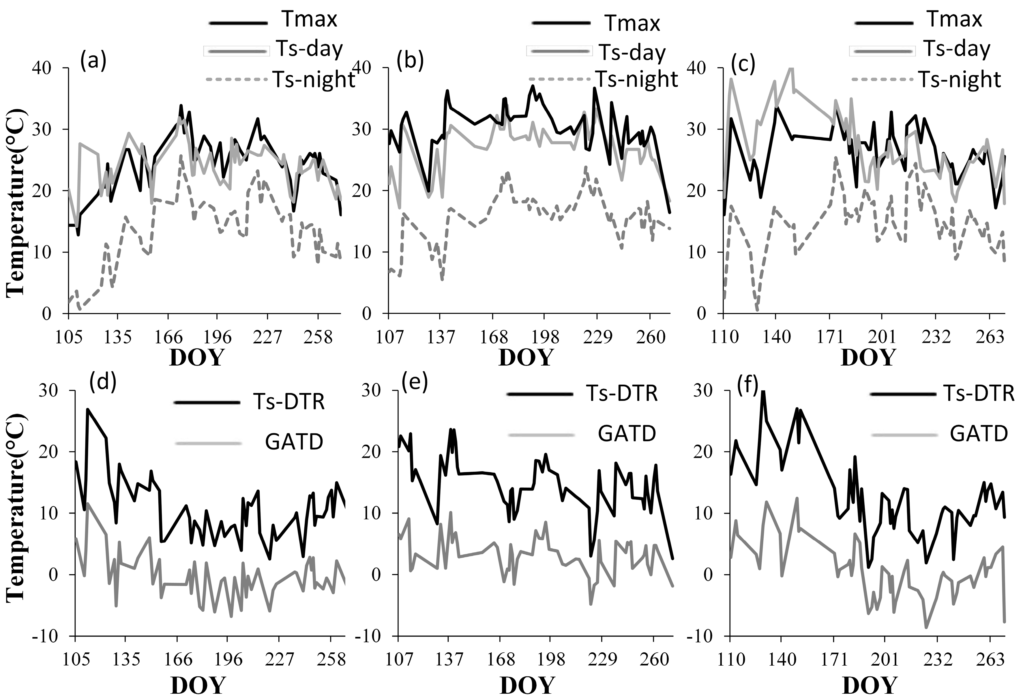
5.4. Spatial and Temporal Patterns

Spatially, relatively lower accuracy was observed in northwestern Iowa, eastern Nebraska and northeastern Illinois (Figure 4). The spatial and temporal patterns of Tmax agree well with the MIDV patterns during the study period. Similar to the result of Landsberg’s [38] study, in the Corn Belt, the Tmax IDV showed a spatial zonal pattern (Figure 8) of increasing with latitude. It was also higher in spring and autumn than summer. The stations with larger Tmax IDV (>2.6) tend to have lower Tmax estimation accuracy (Figure 4 and Figure 8). In addition, the correlation coefficient between Tmax MIDV and Tmax RMSE in individual stations during the study period 2008 to 2012 was 0.41 (p < 0.01) (Figure 9). On the regional scale, the Tmax MIDV from May to September were 3.51 °C, 2.67 °C, 2.17 °C, 2.12 °C, and 2.99 °C, respectively. It also agrees well with the trends of Tmax estimation accuracy temporally, which is also highest in May and lowest in August. For Tmax estimation, there is a trend that higher Tmax IDV resulted in higher Tmax estimation errors (Figure 10a,c). The Ts tended to overestimate Tmax if the Ta of the current day was lower than that of the previous or/and next day and to underestimate Tmax if the Ta of the current day was higher than that of the previous or/and next day (Figure 10a,c). The day-to-day difference of Tmax can reflect the changes of air masses, as well as the sources of air masses and their sources and major paths [38]. Generally, air is mainly heated by land surface, however air masses usually strike the local energy balance. Cool air moving over a warm surface is heated from below and warm air moving over a cool surface is cooled from below [45]. There is a time lag for the establishment of new balance between air and land surface temperature. As a result, before that, with cool air and warm air, LST tends to overestimate and underestimate Ta, respectively, when using LST to estimate Ta.
Figure 8. MIDV of (a) Tmax and (b) Tmin (°C) of the individual stations during 2008–2012 throughout the growing season.
Remotesensing 07 00951 g008
Figure 9. Scatterplot of Tmax MIDV vs. Tmax RMSE (°C), of all individual stations included in this study during 2008 to 2012.
Remotesensing 07 00951 g009
Figure 10. catterplot of estimation error (estimated Ta minus observed Ta) of Tmax (a) and Tmin (b) vs. the IDV of the current day (Equation (3)), and estimation error of Tmax (c) and Tmin (d) vs. the IDV of the next day (Equation (3)), for crop area during 2008–2012 throughout the growing season.
Remotesensing 07 00951 g010
In addition, irrigation might have contribute to the low Tmax estimation accuracy in eastern Nebraska. The relationship between observed and estimated Tmax in this area was examined and it was found that the Ts of these stations (e.g., Columbus 3 NE, Friend 3 E, and Surprise) that are dominated by irrigated crop land, tends to underestimate the Tmax, especially in 2012, due to irrigation. According to the 2007 Census of Agriculture, of approximately 55 million acres under irrigation nationally, about 15% are located in Nebraska (8.56 million acres) [46]. About three out of eight cropland acres in Nebraska are under irrigation [46]. Thus, it is reasonable to expect Ts would underestimate Ta in heavily irrigated landscapes where targeted water applications result in significant cooling effect on the land surface as well as the canopy, as more energy is partitioned to the latent heat flux via evapotranspiration [41]. The air will be cooled after irrigation as well, but compared to the decrease of Ts value, the decrease of Ta is very small.
As for Tmin estimation, there is no apparent relation spatially. In addition, there is no obvious relation between Tmin IDV and Tmin estimation errors (Figure 10b,d). Landsberg [38] stated that, as compared to changes in Tmax, changes in the Tmin are less affected by air masses but much more affected by local conditions such as proximity to water bodies and mountains orographic tendencies for inversion formation, and other environmental characteristics. This may be a possible reason for the low accuracy in Tmin estimation in northwestern Iowa. While at a regional scale, the trends of Tmin MIDV from May to September (2.75 °C, 2.24 °C, 1.87 °C, 2.10 °C, and 2.60 °C, respectively) agree well with that of Tmin estimation accuracy (Figure 3).
There may also be some other possible reasons leading to the low estimation accuracy. Though combining both Ts-day and Ts-night to estimate Tmax reduced the impact of land-cover types and vegetation cover changes, vegetation variables might still have impact on the Ta estimation accuracy. It is shown from Table 2 that by integrating DOY information, the estimation accuracy of models for both Tmax and Tmin were improved, especially in crops areas and forest areas. As vegetation had been variously contributed to latent heat flux, canopy resistance to transpiration [19]. DOY included the information of vegetation cover changes with seasons. Remaining clouds (pixel and sub-pixel) negatively affect the model performance. Though only pixels marked as cloud-free were selected and the cloud cover of the 13-by-13 pixel window was less than 10%, there were still some cloud-contaminated pixels included. Thin or sub-pixel cloud cover detection is difficult [47] and the LST retrieved under these conditions often corresponds to top-of-cloud temperature [4,48]. In addition, most undetected cloud-contaminated LST outliers occur in cloud edges and a large proportion of the pixels with higher errors occurred near identified clouds [33,49]. However, cloud-edge elimination, such as considering a 10-km buffer [48], could limit data availability significantly. Thus, some errors and uncertainty have been brought into this study by cloud contamination in order to collect a sufficient sample size of pixels. Other factors could also explain some of the errors in Ta estimation from Ts. Prihodko and Goward [19] observed deviations of 0.6 °C at horizontal distances of 6-km from a dense spatial ground network of meteorological stations. The temperature in the 13-by-13 windows is quite homogeneous in flat terrain conditions. However, temperature may show larger spatial variations in hilly areas (e.g., the northwest of Iowa) [22].

6. Conclusions

In this study, the relationships between Tmax, Tmin and both daily Ts-day and Ts-night were analyzed and discussed. The results of this study can be considered promising, given the simplicity of the statistical models employed and the high accuracy achieved with RMSE of Tmax estimation 2.27 °C, 2.19 °C and 2.33 °C and RMSE of Tmin estimation 1.76 °C, 1.82 °C and 1.82 °C, for crops, deciduous forest and developed areas respectively.
Interestingly, Ts-night had higher correlation coefficient with daily Tmax than Ts-day in all the three land-cover types. Combining both Ts-day and Ts-night to estimate Tmax achieved even better accuracy than either variable individually. Compared to using only Ts-night, combining Ts-day and Ts-night have little improvement on Tmin estimation accuracy, as Ts-day was not relevant for Tmin estimation. Taken DOY into consideration, slight improvement of both Tmax and Tmin estimation accuracy was observed in crops and forest areas rather than developed areas. Both Ts-day and Ts-night from Terra are better explanatory variables for Tmax, while Ts-night from Aqua is a slight better (~0.2 °C) proxy for Tmin. The models had a general tendency to have lower performance of Tmax estimation in stations located in irrigated land and the areas with higher IDV, but a better performance of Tmax estimation during the period from June to August (the middle of the growing season) than either May or September (the beginning or end of the growing season) due to the spatial and temporal difference of air masses as well as irrigation. While there was no distinct spatial distribution pattern of Tmin estimation across the Corn Belt. Some other factors such as cloud cover and other local conditions might also contribute to the difference of estimation accuracy of Tmin.
As for the TVX method, a wide range of vegetation index (VI) variability in the window, uniform atmospheric forcing and moisture conditions are required to build the regression relation between Ta and VI [19]. But Corn Belt, mostly covered by crops, has small range of VI variability. This study provides a feasible and improved way to estimate Tmax and Tmin in this study area. Through the analysis of Ts and Ta relations over crop, deciduous forest, developed area and the spatial and temporal variability of Ta estimation accuracy in the Corn Belt, the Ts and Ta relations are better understood in this area. A wide range of applications can benefit from this study, especially in agriculture. The estimated Ta can be used as an input for GDD in large area based on remotely sensed data.
Based on the spatial and temporal analysis of Ta estimation accuracy, this work highlighted future possible improvements of Ta based on remote sensing data such as (1) take the changes of current Ta compared to that of previous days and later days, and surface energy balance process into consideration; (2) integrate vegetation variables into Ta estimation model; (3) integrate water stress of vegetation into Ta estimation model.

Acknowledgments

We gratefully acknowledge the use of facilities and equipment provided by the National Drought Mitigation Center (NDMC), The Center for Advanced Land Management Information Technologies (CALMIT) and University of Nebraska-Lincoln (UNL).

Author Contributions

Linglin Zeng carried out the research work, proposed the idea and structure of this manuscript, wrote the majority of the paper. Brain D Wardlow supervised the research and contributed to manuscript organization, writing and revisions. Tsegaye Tadesse, Jie Shan, Michael J Hayes and Deren Li helped with discussions and manuscript revisions. Daxiang Xiang helped with discussions.

Conflicts of Interest

The authors declare no conflict of interest.

References

  1. De Bruin, H.A.R.; Trigo, I.F.; Jitan, M.A.; TemesgenEnku, N.; van der Tol, C.; Gieske, A.S.M. Reference crop evapotranspiration derived from geo-stationary satellite imagery: A case study for the Fogera flood plain, NW-Ethiopia and the Jordan Valley, Jordan. Hydrol. Earth Syst. Sci. 2010, 14, 2219–2228. [Google Scholar]
  2. Gao, H.; Tang, Q.; Shi, X.; Zhu, C.; Bohn, T.J.; Su, F.; Sheffield, J.; Pan, M.; Lettenmaier, D.P.; Wood, E.F.; et al. Water budget record from Variable Infiltration Capacity (VIC) Model. Algorithm Theoretical Basis Document for Terrestrial Water Cycle Data Records. Available online: http://grid1.cos.gmu.edu:8090/OPeNDAPClient/ATBD_Chapter6_doc.pdf (accessed on 1 October 2014).
  3. Lofgren, B.M.; Hunter, T.S.; Wilbarger, J. Effects of using air temperature as a proxy for evapotranspiration in climate change scenarios of Great Lakes basin hydrology. J. Gt. Lakes Res. 2011, 37, 744–752. [Google Scholar]
  4. Benali, A.; Carvalho, A.C.; Nunes, J.P.; Carvalhais, N.; Santos, A. Estimating air surface temperature in Portugal using MODIS LST data. Remote Sens. Environ. 2012, 124, 108–121. [Google Scholar]
  5. Willmott, C.J.; Robeson, S.M. Climatologically Aided Interpolation (CAI) of terrestrial air temperature. Int. J. Climatol. 1995, 15, 221–229. [Google Scholar]
  6. Pinheiro, A.C.T.; Mahoney, R.; Privette, J.L.; Tucker, C.J. Development of a daily long-term record of NOAA-14 AVHRR land surface temperature over Africa. Remote Sens. Environ. 2006, 103, 153–164. [Google Scholar]
  7. Wan, Z.; Zhang, Y.; Zhang, Y.Q.; Li, Z.L. Validation of the land-surface temperature products retrieved from moderate resolution imaging spectroradiometer data. Remote Sens. Environ. 2002, 83, 163–180. [Google Scholar]
  8. Atitar, M.; Sobrino, J.A. A split-window algorithm for estimating LST from Meteosat 9 data: Test and comparison with in situ data and MODIS LSTs. IEEE Geosci. Remote Sens. Lett. 2009, 6, 122–126. [Google Scholar]
  9. Mostovoy, G.V.; King, R.L.; Reddy, K.R.; Kakani, V.G.; Filippova, M.G. Statistical estimation of daily maximum and minimum air temperatures from MODIS Ts data over the state of Mississippi. Geosci. Remote Sens. 2006, 43, 78–110. [Google Scholar]
  10. Lin, S.; Moore, N.J.; Messina, J.P.; de Visser, M.H.; Wu, J. Evaluation of estimating daily maximum and minimum air temperature with MODIS data in east Africa. Int. J. Appl. Earth Obs. Geoinf. 2012, 18, 128–140. [Google Scholar]
  11. Frederick, K.L.; Edward, J.T.; Dennis, G.T. The Atmosphere: An Introduction to Meteorology, 10th ed.; Prentice Hall: Upper Saddle River, NJ, USA, 2006. [Google Scholar]
  12. Goward, S.N.; Dye, D. Global biospheric monitoring with remote sensing. In The Use of Remote Sensing in Modeling Forest Productivity at Scales From the Stand to the Globe; Gholtz, H.L., Nakane, K., Shimoda, H., Eds.; Kluwer Academic: New York, NY, USA, 1997; pp. 241–272. [Google Scholar]
  13. Prince, S.D.; Goetz, S.J.; Dubayah, R.O.; Czajkowski, K.P.; Thawley, M. Inference of surface and air temperature, atmospheric precipitable water and vapor pressure deficit using advanced very high-resolution radiometer satellite observations: Comparison with field observations. J. Hydrol. 1998, 213, 230–249. [Google Scholar]
  14. Stisen, S.; Sandholt, I.; Norgaard, A.; Fensholt, R.; Eklundh, L. Estimation of diurnal air temperature using MSG SEVIRI data in West Africa. Remote Sens. Environ. 2007, 110, 262–274. [Google Scholar]
  15. Zakšek, K.; Schroedter-Homscheidt, M. Parameterization of air temperature in high temporal and spatial resolution from a combination of the SEVIRI and MODIS instruments. ISPRS J. Photogramm. Remote Sens. 2009, 64, 414–421. [Google Scholar]
  16. Cresswell, M.P.; Morse, A.P.; Thomson, M.C.; Connor, S.J. Estimating surface air temperatures, from Meteosat land surface temperatures, using an empirical solar zenith angle model. Int. J. Remote Sens. 1999, 20, 1125–1132. [Google Scholar]
  17. Jang, J.D.; Viau, A.A.; Anctil, F. Neural network estimation of air temperatures from AVHRR data. Int. J. Remote Sens. 2004, 25, 4541–4554. [Google Scholar]
  18. Fu, G.; Shen, Z.X.; Zhang, X.Z.; Shi, P.L.; Zhang, Y.J.; Wu, J.S. Estimating air temperature of an alpine meadow on the Northern Tibetan Plateau using MODIS land surface temperature. Acta Ecol. Sin. 2011, 21, 8–13. [Google Scholar]
  19. Prihodko, L.; Goward, S.N. Estimation of air temperature from remotely sensed surface observations. Remote Sens. Environ. 1997, 60, 335–346. [Google Scholar]
  20. Nemani, R.R.; Running, S.W. Estimation of regional surface resistance to evapotranspiration from NDVI and thermal IR AVHRR data. J. Appl. Meteorol. 1989, 28, 276–284. [Google Scholar]
  21. Zhu, W.; Lű, A.; Jia, S. Estimation of daily maximum and minimum air temperature using MODIS land surface temperature products. Remote Sens. Environ. 2013, 130, 62–73. [Google Scholar]
  22. Vancutsem, C.; Ceccato, P.; Dinku, T.; Connor, S.J. Evaluation of MODIS land surface temperature data to estimate air temperature in different ecosystems over Africa. Remote Sens. Environ. 2010, 114, 449–465. [Google Scholar]
  23. Karnieli, A.; Dall’Olmo, G. Remote sensing monitoring of desertification, phenology, and droughts. Manag. Environ. Q. Int. J. 2003, 14, 22–38. [Google Scholar]
  24. Sun, Y.J.; Wang, J.F.; Zhang, R.H.; Gillies, R.R.; Xue, Y.; Bo, Y.C. Air temperature retrieval from remote sensing data based on thermodynamics. Theor. Appl. Climatol. 2005, 80, 37–48. [Google Scholar]
  25. Gallo, K.; Hale, R.; Tarpley, D.; Yu, Y. Evaluation of the relationship between air and land surface temperature under clear- and cloudy-sky conditions. J. Appl. Meteorol. Climatol. 2011, 50, 767–775. [Google Scholar]
  26. Shah, D.B.; Pandya, M.R.; Trivedi, H.J.; Jani, A.R. Estimating minimum and maximum air temperature using MODIS data over Indo-Gangetic Plain. J. Earth Syst. Sci. 2013, 122, 1593–1605. [Google Scholar]
  27. McMaster, G.S.; Wilhelm, W.W. Growing degree-days: One equation, two interpretations. Agric. For. Meteorol. 1997, 87, 291–300. [Google Scholar]
  28. USDA. Crop Production 2012 Summary. Available online: http://usda01.library.cornell.edu/usda/current/CropProdSu/CropProdSu-01–10–2014.pdf (accessed on 28 May 2014).
  29. EOSDIS. Available online: http://reverb.echo.nasa.gov/reverb/ (accessed on 01 October 2014).
  30. National Climatic Data Center. Available online: http://www.ncdc.noaa.gov/ (accessed on 01 October 2014).
  31. Cropland Data Layers. Available online: http://www.nass.usda.gov/research/Cropland/SARS1a.htm (accessed on 01 October 2014).
  32. Pervez, M.S.; Brown, J.F. Mapping irrigated lands at 250-m scale by merging MODIS data and national agricultural statistics. Remote Sens. 2010, 2, 2388–2412. [Google Scholar]
  33. The Regional and Mesoscale Meteorology Branch. Solar Zenith Angle algorithms. Available online: http://rammb.cira.colostate.edu/wmovl/vrl/tutorials/euromet/courses/english/nwp/n5720/n5720005.htm (accessed on 18 November 2014).
  34. Wan, Z.; Zhang, Y.; Zhang, Q.; Li, Z.L. Quality assessment and validation of the MODIS global land surface temperature. Int. J. Remote Sens. 2004, 25, 261–274. [Google Scholar]
  35. Wan, Z.; Li, Z.L. Radiance-based validation of the V5 MODIS land-surface temperature product. Int. J. Remote Sens. 2008, 29, 5373–5395. [Google Scholar]
  36. Rizzoli, A.; Neteler, M.; Rosà, R.; Versini, W.; Cristofolini, A.; Bregoli, M. Early detection of TBEv spatial distribution and activity in the Province of Trento assessed using serological and remotely-sensed climatic data. Geospat. Health 2007, 1, 169–176. [Google Scholar]
  37. Janssen, P.H.M.; Heuberger, P.S.C. Calibration of process-oriented models. Ecol. Model. 1995, 83, 55–66. [Google Scholar]
  38. Landsberg, H.E. Interdiurnal Variability of Pressure and Temperature in the Coterminous United States; Technical Paper No. 56; U.S; Department of Commerce: Washington, DC, USA, 1966. [Google Scholar]
  39. Rosenthal, S.L. The interdiurnal variability of surface-air temperature over the North Atlantic Ocean. J. Meteorol. 1960, 17, 1–7. [Google Scholar]
  40. Parton, W.J.; Logan, J.A. A model for diurnal variation in soil and air temperature. Agric. Meteorol. 1981, 23, 205–216. [Google Scholar]
  41. Monteith, J.; Unsworth, M. Principles of Environmental Physics; Academic Press: London, UK, 2007. [Google Scholar]
  42. Collatz, G.J.; Bounoua, L.; Los, S.O.; Randall, D.A.; Fung, I.Y.; Sellers, P.J. A mechanism for the influence of vegetation on the response of the diurnal temperature range to a changing climate. Geophys. Res. Lett. 2000, 27, 3381–3384. [Google Scholar]
  43. Dai, A.; Trenberth, K.E.; Karl, T.R. Effects of clouds, soil moisture, precipitation, and water vapor on diurnal temperature range. J. Clim. 1999, 12, 2451–2473. [Google Scholar]
  44. Easterling, D.R.; Horton, B.; Jones, P.D.; Peterson, T.C.; Karl, T.R.; Parker., D.E.; Salinger, M.J.; Razuvayev, V.; Plummer, N.; Jamason, P.; et al. Maximum and minimum temperature trends for the globe. Science 1997, 277, 364–367. [Google Scholar]
  45. Weather Almanac. Available online: http://www.weatherexplained.com/Vol-1/Weather-Fundamentals.html (accessed on 18 May 2014).
  46. Johnson, B.; Thompson, C.; Giri, A.; NewKirk, S.V. Nebraska Irrigation Fact Sheet. Available online: http://agecon.unl.edu/c/document_library/get_file?uuid=a9fcd902-4da9-4c3f-9e04-c8b56a9b22c7&groupId=2369805&.pdf (accessed on 28 May 2014).
  47. Ackerman, S.; Strabala, K.; Menzel, P.; Frey, R.; Moeller, C.; Gumley, L. Discriminating clear sky from clouds with MODIS. J. Geophys. Res. 1998, 103, 141–157. [Google Scholar]
  48. Neteler, M. Estimating daily land surface temperatures in mountainous environments by reconstructed MODIS LST data. Remote Sens. 2010, 2, 333–351. [Google Scholar]
  49. Czajkowski, K.P.; Goward, S.N.; Stadler, S.; Walz, A. Thermal remote sensing of near surface environmental variables: Application over the Oklahoma Mesonet. Prof. Geogr. 2000, 52, 345–357. [Google Scholar]

