Article

Assessing Handheld Mobile Laser Scanners for Forest Surveys

1
Faculty of Engineering, The University of Nottingham, Nottingham NG7 2RD, UK
2
RPS, Nelson House, Axminster, Devon EX13 5AX, UK
3
Laser Mapping, Unit 1 Moorbridge Court, Bingham NG13 8GG, UK
4
School of Life Sciences, The University of Nottingham, Nottingham NG7 2RD, UK
*
Author to whom correspondence should be addressed.
Current address: OXBOTICA Ltd, 23 Banbury Road, Oxford, OX2 6NN, UK
Remote Sens. 2015, 7(1), 1095-1111; https://0-doi-org.brum.beds.ac.uk/10.3390/rs70101095
Submission received: 29 August 2014 / Accepted: 12 January 2015 / Published: 19 January 2015

Abstract

:
A handheld mobile laser scanning (HMLS) approach to forest inventory surveying allows virtual reconstructions of forest stands and extraction of key structural parameters from beneath the canopy, significantly reducing survey time when compared against static laser scan and fieldwork methods. A proof of concept test application demonstrated the ability of this technique to successfully extract diameter at breast height (DBH) and stem position compared against a concurrent terrestrial laser scan (TLS) survey. When stems with DBH > 10 cm are examined, an HMLS to TLS modelling success rate of 91% was achieved with the root mean square error (RMSE) of the DBH and stem position being 1.5 cm and 2.1 cm respectively. The HMLS approach gave a survey coverage time per surveyor of 50 m2/min compared with 0.85 m2/min for the TLS instrument and 0.43 m2/min for the field study. This powerful tool has potential applications in forest surveying by providing much larger data sets at reduced operational costs to current survey methods. HMLS provides an efficient, cost effective, versatile forest surveying technique, which can be conducted as easily as walking through a plot, allowing much more detailed, spatially extensive survey data to be collected.

Graphical Abstract

1. Introduction

The use of aerial laser scanning (ALS) has revolutionised our ability to collect forest inventory data over large areas and its use can produce substantial cost reductions when compared against traditional forest surveys [1]. Nevertheless, although the use of ALS surveys has increased dramatically in recent years [2], permanent sample plots within forest sites are still needed for accurate measurement of below canopy structural parameters and for the calibration of forest models developed from ALS [3,4,5]. There is also a need to understand how forests operate at finer detail beneath the canopy, such as within understorey microhabitats [6], and it is in this area that ground-based surveying techniques can play a pivotal role.
Recent developments in the speed, accuracy and affordability of terrestrial laser scanning (TLS) systems have opened the possibility of major enhancements to existing studies by providing detailed information on three-dimensional forest structures [7]. This is achieved through single scans with a fixed viewpoint [8] or by combining the results of multiple scans to recreate complex habitats [9,10]. Such new tools allow replicable controlled measures of many forest features relevant to ecologists, environmental scientists and foresters, including the dimensions and heterogeneity of canopies, size and distribution of canopy gaps, leaf area index (LAI—leaf area per unit ground area) and total surface area of stems and leaves.
At the present time TLS, while demonstrating the potential of the technology, has been typically used for the measurement of small-scale sample plots within larger woodland sites. A large obstacle to the uptake of TLS for larger-scale forest monitoring projects is the time and costs associated with building point clouds of sufficient size to adequately describe the forest environment. With line-of-sight often limited to several metres, multiple scan locations are required to produce data sets that can be used for accurate feature extraction [11]. This limitation means that a TLS generated point cloud describing an entire woodland plot is currently too time-consuming and costly to be considered for operational purpose.
Mobile laser scanning (MLS) systems offer a potential solution to the problem of creating ground-based point clouds with the necessary geospatial extent whilst maintaining accuracy [12] and minimising time and cost. MLS is a technology that uses a navigation module to determine the position of a laser whilst the laser takes measurements of the environment. A typical MLS system combines a laser scanning instrument, a moving platform and a positioning and orientation determination device such as a Global Navigation Satellite System (GNSS) receiver and inertial measurement unit (IMU). This configuration limits their use to relatively open environments, such as highways and infrastructure corridors. MLS systems are currently predominantly mounted on cars for urban mapping [13], with the technology being increasingly used in agro-forestry [14]. Liang et al. (2014) [15] and Liang et al. (2013) [16] have also demonstrated a MLS instrument mounted on an all-terrain vehicle and as a backpack carried personal laser scanning system (PLS), for use within forest plots.
In this study the potential for a handheld mobile laser scanner (HMLS) to provide point clouds of similar precision and accuracy to those currently being produced through TLS applications was explored. An assessment of laser scan survey times when compared against the field survey method was also carried out. The survey was completed in a complex, semi-natural woodland stand rather than managed woodland with roads and paths running through it. The aim was to address four main questions: (1) Can TLS measurements of forests be replicated using HMLS; (2) does the use of HMLS provide any advantages in practical ease over TLS or field survey methods; (3) are any novel measurements available; and (4) what are the remaining challenges for the application of HMLS in forest monitoring.

2. Methods

2.1. Instrumentation

2.1.1. FARO Focus 3D
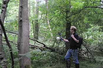
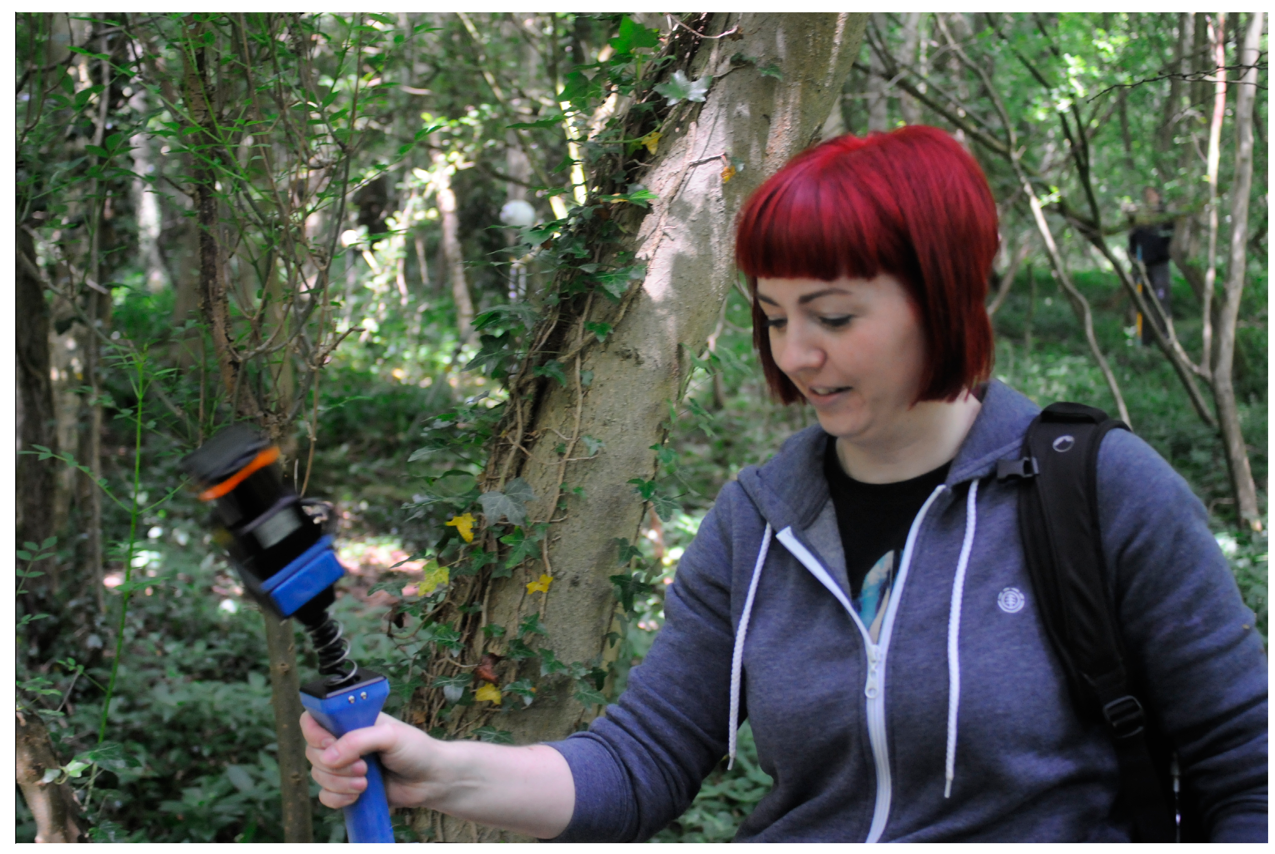
The FARO Focus 3D [17] is a commercially available TLS instrument that has been designed for use in architecture or civil engineering projects. It is lightweight (5.2 kg) and small (24 × 20 × 10 cm) making it more appropriate for forest surveying than some of the larger instruments currently available. The instrument is a phase-based lidar with a working range of up to 120 m and a maximum point collection of 9.76 × 10⁵ per second. For each point return XYZ coordinates and a reflectance value (intensity of returning beam) are given. Using the internal colour camera RGB values for each return can also be acquired. The manufacturer’s stated ranging error is up to ±2 mm, this being the measurement error at around 10 m and 25 m, one sigma.
FARO registration and survey spheres are used to provide tie points to join scans from multiple set-ups. Using multiple survey positions minimises the point occlusion from shadowing and allows for greater point density within the plot [18]. When using multiple survey positions, care needs to be taken to ensure the survey spheres are visible from multiple scanner locations.
The FARO Focus 3D is a system that has been previously tested for its potential in forest mapping [19].

2.1.2. ZEB1

New to the MLS family is the ZEB1 handheld mobile laser scanner (Figure 1). Instead of using GNSS within the navigation module the ZEB1 makes use of a technology taken from the robotics community, simultaneous localisation and mapping (SLAM). The concept of SLAM is that a robot can be placed in an unknown environment and has the ability to create a map and then navigate to a particular destination. An introduction to the science can be read in [20,21]. The mapping module forms the basis for use within the ZEB1. The fact that the ZEB1 is lightweight (0.7 kg) and has no reliance on GPS makes it an ideal data capture method for inaccessible areas such as under tree canopies and indoors [22].
The ZEB1 consists of a laser scanner and low-cost IMU, both of which are positioned on top of a spring which has been designed to have the resonant frequency of the average human gait [23]. As the user carries the ZEB1 through the environment, the scanner head rocks back and forth creating a 3D field of measurement with data being captured at the speed of movement. The algorithm used to calculate the position and orientation of the scanner head (referred to as the trajectory) processes IMU and laser data from the ZEB1 using a moving time window through the raw data. As new data is added the algorithm uses a linearised model to minimise the error in the IMU measurements along with minimising the correspondences between the 3D point cloud data for the respective time segment. The correspondences for the 3D point cloud are minimised using a technique similar to the iterative closest point algorithm [24], but instead of solving for one rigid transformation as in TLS the matching take place periodically linked to the motion of the scanner head [23]. The final smoothed trajectory is used to compute the coordinates for the full 3D point cloud. The ZEB1 converges on the best solution when the scanned area contains many unique features, which can be identifiable in consecutive rocks of the scanner. The manufacturer’s stated measurement error is ±30 mm at a range of 0.1 m to 10 m.
Figure 1. ZEB1 handheld mobile laser scanner in operation for forest mapping.
Remotesensing 07 01095 g001
The ZEB1 instrument works best where all surfaces are facing in multiple directions in the environment, such as indoors. The SLAM solution is based on the theory that the same objects are viewed from multiple directions as the system moves through the environment; measurements to these objects are then used to calculate position. This requires that objects used for positioning remain static. The ZEB1 has been designed to cope with some movement in the environment and the point correspondence step will remove many moving objects from the solution [21]. An environment under a dense tree canopy provides many static features (large stems) as well as less static features (foliage, small stems and understorey). Using a SLAM-based device for data capture in dense forest may prove difficult due to foliage motion in some weather conditions.

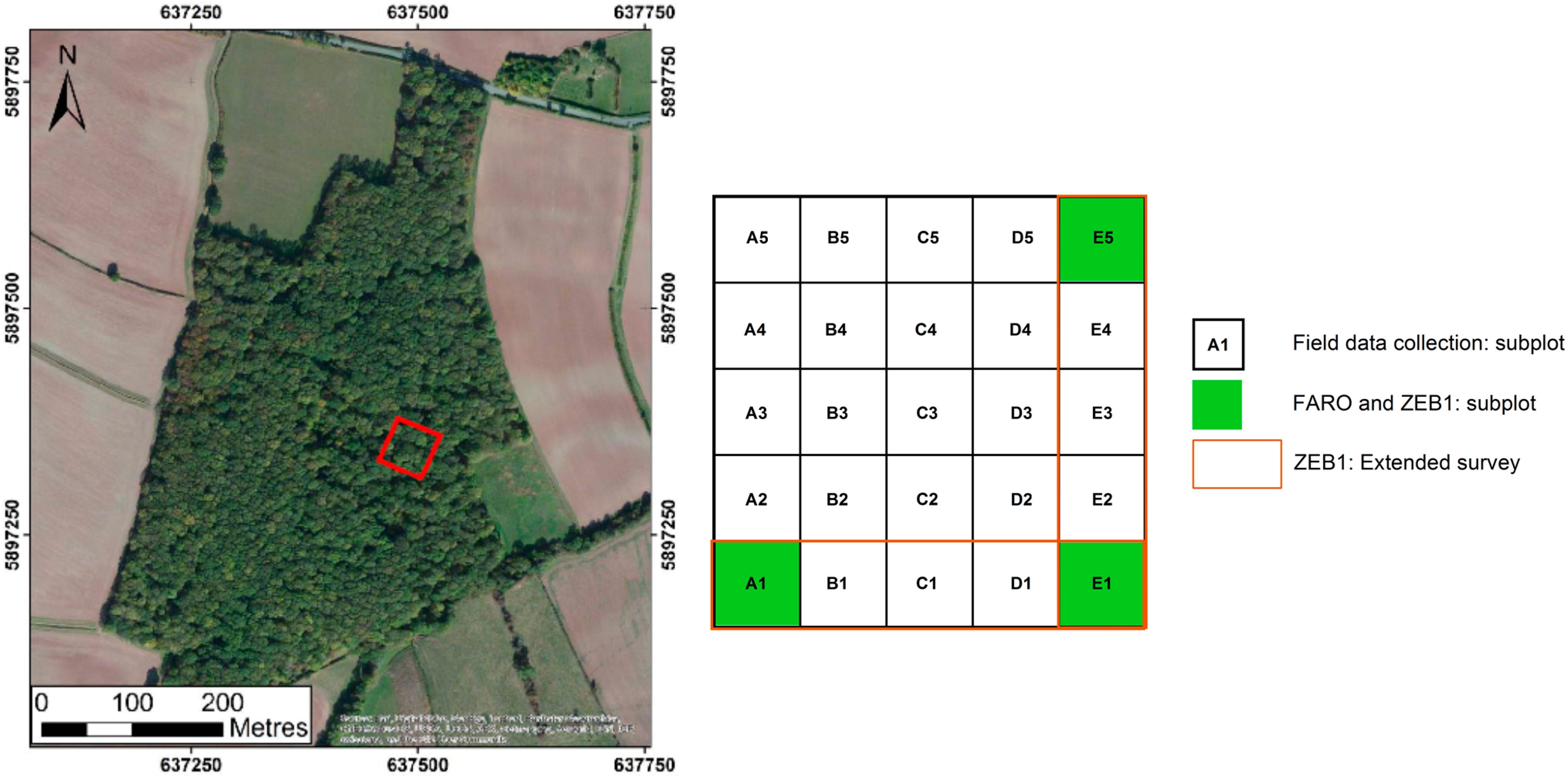
2.2. Test Site Description and Data Collection

Kirton Wood SSSI, Nottinghamshire (SK 762798), is a 47.8 ha ash dominated woodland. It is managed by Nottinghamshire Wildlife Trust.
Field survey data were collected from a previously constructed survey area within Kirton Wood measuring 50 m × 50 m. The survey area is divided into 25 subplots each measuring 10 m × 10 m (Figure 2), three of which were used to test the different scanning methods. The plot site is semi-natural ash, elm woodland and has been left to develop largely undisturbed since the 1930s. The shrub community includes field maple, hawthorn and hazel with dense ground flora present. A description of the three subplot sites as collected during the field study is given in Table 1.
Figure 2. Kirton Wood survey plan showing location of test site within woodland and subplot position (image source: Esri, DigitalGlobe, GeoEye, i-cubed, Earthstar Geographics, CNES/Airbus DS, USDA, USGS, AEX, Getmapping, Aerogird, IGN, IGP, swisstopo, and the GIS User Community).
Remotesensing 07 01095 g002
Table 1. Description of subplots used at test site. DBH: diameter at breast height.
PlotDominant SpeciesSecondary SpeciesDBH Maximum (cm)DBH Mean (cm)Stem Density Stems/m2
A1hawthornash, dogwood, elm23.55.60.79
E1hazelhawthorn, elm, ash, maple25.45.30.65
E5hawthornelm, ash45.38.70.27
The weather on the day of the survey was very good with clear skies and low wind. As a consequence, there was no wind disturbance within the woodland plot with the environment being described as static. These were ideal conditions to test the ZEB1.
Figure 3. Trajectory for HMLS survey of (a) subplot A1 and (b) zone between subplots.
Remotesensing 07 01095 g003
For the main ZEB1 and FARO surveys three corner subplots (A1, E1 and E5) were selected from the Kirton Wood field survey area. The subplots were chosen to be non-contiguous allowing for work to be carried out with the minimum effect of trampling within the plot area. To test survey data collection rates with the ZEB1, the zones between the corner subplots were also scanned in an extended survey (Figure 3).

2.2.1. FARO Focus 3D Data Collection

At each subplot location three scans were obtained using the FARO Focus 3D. This is a common method for collecting scan data in woodland plots (known as multiple scan mode) whereby three scan locations are positioned around the subplot increasing scan overlap and decreasing point occlusion, whilst not greatly increasing the time spent in the field [18]. The multiple scan mode was chosen over a single scan approach as previous studies have shown that the single scan method fails to identify up to 32% of trees in a sample plot [16]. Two large, white, highly reflective target spheres (Ø 0.2 m) and five smaller registration spheres (Ø 0.14 m) were used to produce the known points needed for point cloud registration. The spheres were distributed to give line-of-sight to the scanner positions and to maintain good geometric spread allowing for a more stable point cloud registration [25].
FARO Focus 3D data was collected at each scan location with a spatial resolution of 7.67 mm at 10 m. The scans covered a field of view 360° in the horizontal and 305° in the vertical with full colour panoramic photographs obtained using the instrument’s internal camera. Using these set up specifications an individual subplot area could be surveyed in one hour. This time includes carrying the equipment to site or between subplots, identifying suitable scan locations, positioning survey spheres so they are visible from multiple scan locations and acquiring the scan data with photographs.

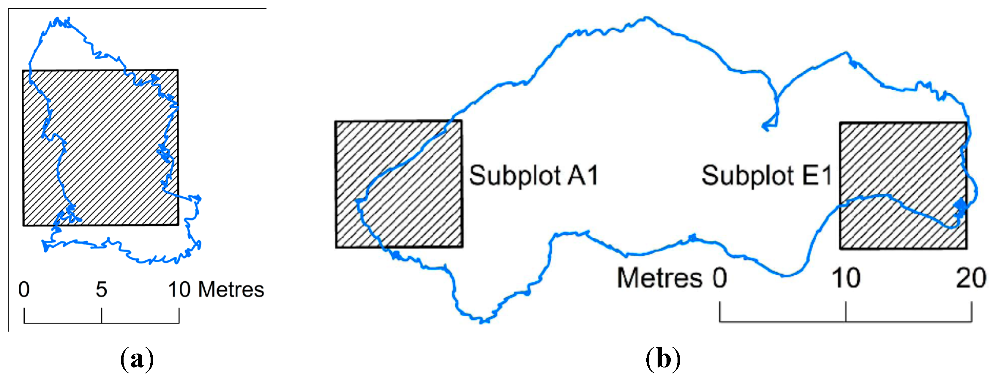
2.2.2. ZEB1 Data Collection

ZEB1 data was acquired at each of the three survey subplots with the user slowly walking across the subplot. A free walking method was used to cover the subplot and where possible the user walked in “straight lines” up and down (obstacles were avoided) with the instrument remaining at breast height throughout (Figure 1). The trajectory path for subplot A1 can be seen in Figure 3a. The survey was completed using a closed loop by starting and ending at the same point. Data collection for each subplot was completed in less than five minutes, including a stationary period at the beginning and end of each scan, which must be completed for initialisation of the system.
In addition to the three subplots surveyed the ZEB1 was used to collect data between subplots A1 and E1 and between subplots E1 and E5, zones of approximately 500 m2 (Figure 2). These data sets were collected to appraise the ability of the handheld system to quickly produce large point clouds, with the same area estimated to take over four hours to collect using the FARO Focus 3D. The trajectory path for this data collection between subplots A1 and E1 can be seen in Figure 3b.
The survey path taken during handheld surveying is critical when considering the usefulness of the method for producing point clouds of the required point accuracy and density. The manufacturers of the ZEB1 state a swath distance of no more than 30 m. In this trial a swath of 5 m was attempted within the subplot areas, with the swath distance in the extended survey between subplots being increased to 20 m.

2.2.3. Field Survey Data Collection

Data were collected one subplot at a time with a team of four ecologists working over two days in October 2008. Diameter at breast height (DBH) was recorded in mm using a standard measuring tape for every stem ≥1 cm. In addition to stem DBH, species and status (dead or alive) were also recorded. Stem positions were calculated using the method of intersection from distance measurements taken to two corner markers within each subplot. The accepted errors for field survey data collection using this method are at the decimetre level [26].

2.3. Laser Scanner Measurement Processing

2.3.1. FARO Focus 3D

For each sample plot the individual FARO scans were registered using the “Scene” laser scanner software [27]. This is designed for registration and processing. Filters were used on the point cloud to remove any likely sources of noise or stray points. Any return with a reflectance value of less than 300 was removed from the data set, this value being the default filter used to remove point noise within the Scene software. Reflectance values for the FARO Focus 3D are given within the range 0 to 2047, which is manufacturer dependent. Additionally, for each scan return a distance from a point to its nearest neighbours within the surrounding area is determined. If over 50% of a point’s neighbouring returns are at a range of more than 2 cm the return is classified as an outlier and removed. This is a standard filter used within Scene software for the removal of stray points.

2.3.2. ZEB1

Once the data had been captured using the ZEB1, it was uploaded to the 3D Laser Mapping secure servers for processing. The data was processed on the servers at a timing ratio of 1:1, with five minutes of data collection taking five minutes to process. The data processing is charged on a pay-as-you-go basis, based on the distance travelled during data collection. Subplot A1 was processed online at a cost of £6.08, with the total online processing for this trial costing £47.78. Once processed the data was downloaded in the .las delivery format, which is compatible with a variety of point cloud software. The returned data was in a local coordinate reference system (CRS) based on the start position of the survey.
A condition value along the ZEB1 survey path is also provided through the online processing. This is a value calculated during ZEB1 processing representing the correspondences created during the matching process and relates to the quality of the matching in the output point cloud. It takes into consideration the orientation and compatibility of the correspondences used and can be used as an indication of how reliable the matching process has been throughout data collection. A poor condition is considered to be a value under 0.2. For this trial condition values ranged from 0.5 to 0.8 therefore the quality of the matched points is considered high.

2.3.3. Transformation to Local Coordinate System

For this study the local coordinate system of the ZEB1 point cloud became the reference for comparison with the FARO point cloud, allowing for direct comparison of the two lidar data sets within the same model space. To enable co-registration all points on the survey spheres (see Section 2.2.1) from the ZEB1 point cloud were isolated and modelled enabling a centroid coordinate to be determined. This was completed using the Leica Cyclone software [28]. The centroid coordinates were then used as control points for registering the scans. Results for the co-registration can be seen in Table 2. Subplots A1 and E1 show mean distance errors of 4 and 3 mm respectively, subplot E5 shows mean distance errors of 16 mm. Registration errors for the three subplots all fall within acceptable levels with 16 mm planimetric error not considered significant in ecological studies [29]. The variation in co-registration errors does however highlight the importance of redundancy when registering scans using targets [25,30]. Only three common survey spheres could be modelled between scan locations for subplot E5, giving little redundancy, whereas for both subplots A1 and E1, five common survey spheres were successfully modelled.
Table 2. Co-registration errors using sphere centroid coordinates.
SubplotNumber of Control PointsMean Distance Error (mm)Min Distance Error (mm)Max Distance Error (mm)
A15426
E153115
E5316940

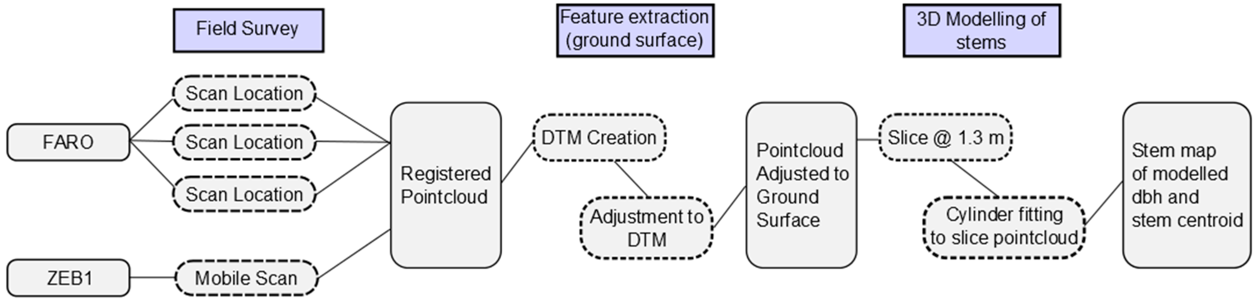
2.4. Feature Extraction

The process of surface creation and adjustment was automated through the use of a Python script utilising the spatial analyst library of ESRI ArcMap. This allowed the registered point cloud from both the FARO and ZEB1 data sets to be processed identically (Figure 4). A digital terrain model was created first and all heights adjusted to height above ground. Slices were taken through each subplot data set at a height of 1.2 m and 1.4 m. Stem mapping and DBH estimations were then performed on these 20 cm slices.
Leica Cyclone software was used to model the stems from which centroid estimations and DBH values could be extracted. Using the sliced data sets, cylinders were fitted to all stem objects (stem objects being selected as showing semi-circular to circular shape in cross section) for both FARO and ZEB1 data sets. This was a manual process. Each cylinder was then isolated and its DBH and centroid at 1.3 m above ground determined.
Figure 4. Workflow for data collection and processing.
Remotesensing 07 01095 g004

2.5. Analysis

For the analysis of results the ZEB1 data set was evaluated against the FARO, which was considered as the control model. This provides a direct comparison of the HMLS approach to forest surveying compared to TLS. The time taken and resultant survey coverage for both laser scan methods and the field survey were also assessed.
The results of the stem modelling were assessed on objects that could be positioned in the FARO data set. Omission differences are where stems are present in the control data set, but not in the model. Commission differences are those where stems are not present in the control, but are in the model [31]. Accuracies of the stem mapping and DBH estimations were gauged using root mean squared error (RMSE), relative RMSE, bias and relative bias:
R M S E =   i = 1 n ( X o b s , i   X m o d e l , i ) 2 n
r e l a t i v e   R M S E =   R M S E x ¯
B i a s =   1 n i = 1 n ( X o b s , i   X m o d e l , i )
r e l a t i v e   B i a s =   B i a s x ¯
where obs,i is the ith observation, model,i is the ith model, x ¯ is the mean of model values, and n is the number of estimations.

3. Results

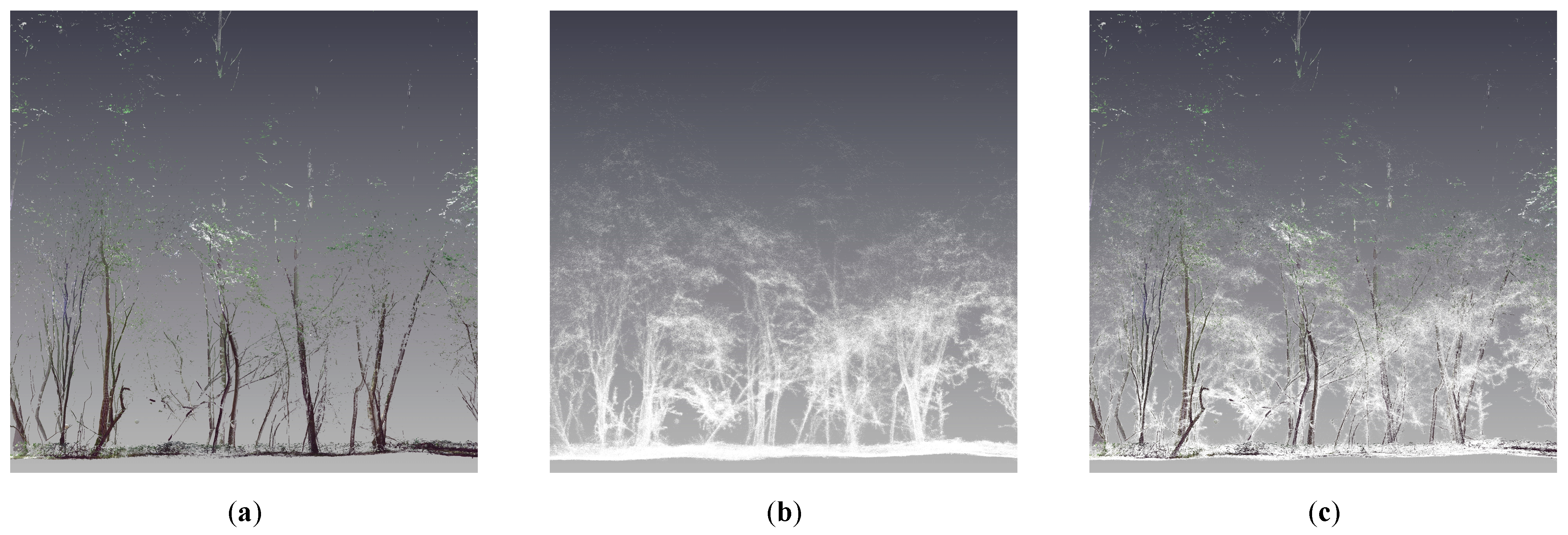
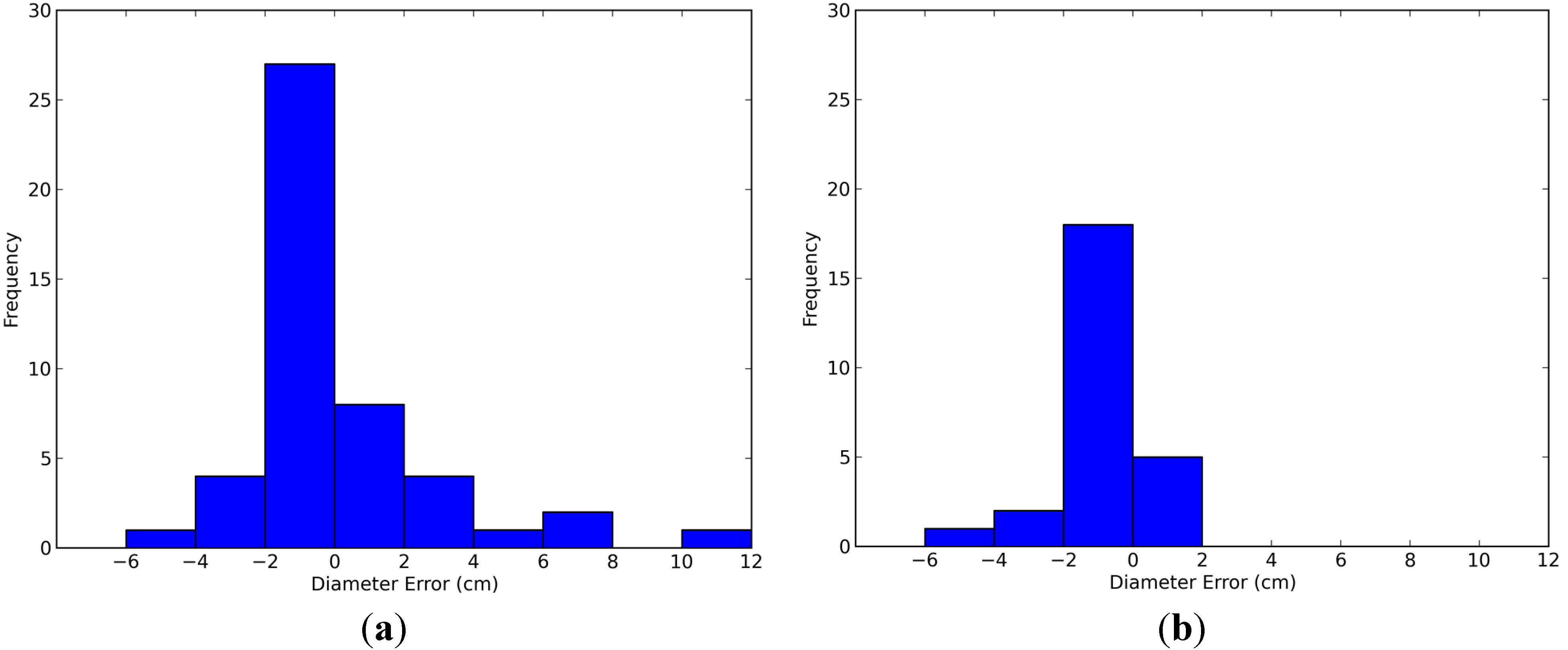
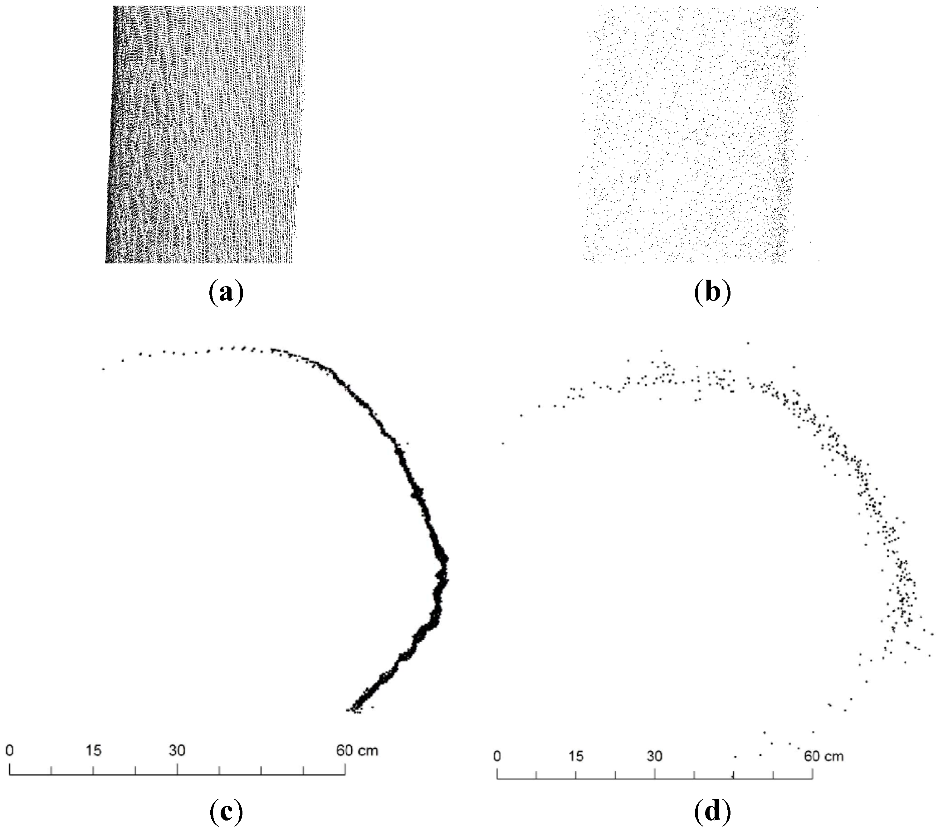
3.1. Direct HMLS to TLS Comparison

Using the FARO data set 54 stems were modelled across all three subplots with the minimum/maximum DBH estimates being 3 cm and 45 cm respectively. Using the ZEB1 data set 49 stems were modelled across all three subplots with minimum/maximum DBH estimates being 5 cm and 45 cm respectively (Table 3). This represents an omission difference of 9% for the ZEB1 compared to the FARO. The results of the DBH estimations and stem mapping can be seen in Table 4 with point cloud comparisons seen in Figure 5 and the distribution of DBH estimation differences seen in Figure 6.
The processing times are similar with both the FARO and ZEB1 once the point clouds have been produced. The FARO registration processing times will vary considerably dependent on influences such as density of woodland, location of targets, etc. The ZEB1 registration processing is approximately equal to the data capture time.
Table 3. Stem modelling results for ZEB1 against FARO.
Subplot FARO Stems ModelledZEB1 Stems Modelled Omission Difference
A123219%
E113128%
E5181611%
Table 4. Accuracies of diameter at breast height (DBH) and stem positioning.
TypeFilterRMSE (cm)Relative RMSE (%)Bias (cm)Relative Bias (%)
SubplotSubplotSubplotSubplot
AllA1E1E5AllA1E1E5AllA1E1E5AllA1E1E5
PlanNone3.12.63.13.5----2.32.02.52.3----
PlanØ > 10 cm2.11.92.41.7----1.71.52.11.5----
PlanØ < 10 cm3.93.24.54.3----2.82.63.72.8----
DBHNone2.93.52.91.9232920170.30.50.30.02.44.62.2−0.3
DBHØ > 10 cm1.51.51.80.9991150.9−1.2−0.7−0.6−5.6−7.4−4.4−3.2
DBHØ < 10 cm3.94.84.82.3466975331.62.53.40.319.535.653.64.3
Figure 5. Point cloud comparisons for (a) FARO (b) ZEB1 and (c) combined data sets.
Remotesensing 07 01095 g005
Figure 6. Distribution of DBH estimation differences between ZEB1 and FARO values with (a) no filter and (b) DBH > 10 cm.
Remotesensing 07 01095 g006

3.2. Comparison of Laser Scanning Survey Times against Field Survey Method

Survey times were recorded and can be seen in Table 5. For the static lidar survey a 10 m × 10 m subplot was completed by two operators in thirty minutes using the FARO system, although if taking into account walking between plot sites and setting up this time is extended to one hour. For the handheld approach, each 10 m × 10 m subplot was surveyed by one person in five minutes. In addition, using the ZEB1 it was possible to traverse the area between subplot sites (Section 2.2) and collect the survey data in little over ten minutes. For the field survey data collection, the Kirton Wood test area (50 m × 50 m) was surveyed by a team of four ecologists over two days.
Table 5. Survey times.
InstrumentPersonnelArea (m2)Time Taken (min)Survey Coverage per Surveyor m2/min
FARO2100600.85
ZEB11100520
ZEB115001050
Field survey4250014400.43
Additional processing time was required for both the ZEB1 and FARO methods, with the field survey being completed on site.

4. Discussion

4.1. Can TLS Measurements Collected for Forest Inventory be Replicated Using HMLS?

The data set and resultant point cloud captured using the ZEB1 was used to extract DBH and stem position information with RMSE of 1.5 cm and 2.1 cm, respectively, when compared against data sets collected using TLS survey techniques and examining stems with a DBH > 10 cm (Table 4).
The handheld approach allows the user to easily direct the scanner toward points of interest and can capture data from the whole survey area, rather than at three set-up points as is usual with a static survey. In this test the user walked steadily through the plot collecting data, but a more directed survey aiming the scanner at all stems may increase modelling accuracy and reduce omission errors. A slower operational gait may also allow for a higher resolution point cloud creation, something that needs to be examined in further trials of the hardware. This is a proof of concept study, which would allow a more vigorous methodology to be developed in future trials.
The cases of stem omission in the ZEB1 data set were caused by insufficient points returned from the handheld system to accurately describe the surface of a stem. These instances caused a modelling error in the Cyclone software and can be classed as complete modelling failure. Omission errors can be caused by point occlusion within the point cloud. Shadowing is a main factor in point occlusion, which can increase in areas of high stem density and increased understorey.
Both plan positioning and DBH estimations show greater errors when stems of DBH < 10 cm are examined (Table 4). For stems with DBH < 10 cm the smaller surface area of the target results in fewer point returns and therefore fewer data from which the stem surface can be modelled. With the most important element of aboveground biomass being trees of DBH > 10 cm [32] the use of a filter to eliminate smaller stems and saplings is a practice used in forest modelling [33]. Removing stems with DBH < 10 cm results in increased accuracy for the plan position and DBH estimations. If the intended application is to assess total basal area then the aggregate effect of these DBH errors will be to add a little more uncertainty to the total value while saving a large amount of survey time.
The manufacturer’s stated accuracies differ greatly for the two instruments with stated accuracies being ±2 mm for the FARO and ±30 mm for the ZEB1. The reduction in point accuracy when using the ZEB1 comes with an increase in data collection efficiency, so this is a trade-off that would need to be assessed for individual survey needs.
DBH estimations show predominance toward underestimation using the handheld system when compared against the FARO (Figure 6). The lower DBH estimations from the ZEB1 instrument are possibly due to the modelling methodology not accounting for the increased point noise seen within the ZEB1 data set [34]. When extracting surfaces the Cyclone software fits cylinders to the inner diameter of the point cloud. With increased surface noise that can be seen in the ZEB1 approach (Figure 7), this may result in decreased diameter estimations. Surface noise may be caused by multiple sources such as object surface texture and registration accuracy, but with decreased measurement accuracy the ZEB1 does contain significantly more uncertainty when modelling surfaces. Using a different modelling methodology may take into account the surface noise and minimise bias.
The trial highlights the potential for a handheld system to replace static lidar for surveying complex, difficult to access forest plots, for recording DBH and plan position. When examining stems with a DBH > 10 cm the utilisation of a handheld survey approach provides an acceptable accuracy (for most forestry applications) in DBH and position estimations whilst increasing the possible survey extent. The method may not, however, currently provide the required surface accuracy for the reconstruction of trees for precise volume/biomass estimations, or the required DBH and position accuracies when examining stems with a DBH of < 10 cm.
Figure 7. Point cloud stem comparisons for (a,b) side view of FARO and ZEBl; (c,d) planar view—10 cm slice of FARO and ZEB1.
Remotesensing 07 01095 g007
There is potential for more cost-effective surveys using the handheld approach. With reduced survey time comes the associated reduction in operational costs. There are also reduced hardware costs, with a ZEB1 instrument costing £14,000. This is currently less than a TLS instrument, which can range from £25,000 to £80,000 depending on manufacturer. Processing costs are more difficult to compare between the two systems with initial processing of the ZEB1 data being priced on a per metre basis, currently approximately £200 per kilometre of survey path. TLS systems do not have this external processing cost, although registration has to be completed in-house.

4.2. Does the Use of HMLS Provide any Advantages in Practical Ease?

Of the methodologies tested the handheld laser scanner showed a much greater area of coverage per hour of survey than the TLS approach or the field survey (Table 5 and Figure 8), significantly reducing the time spent at the forest plot. From the subplot surveys it is estimated that the ZEB1 approach is approximately 12 times faster than if using a TLS. This is comparable with James & Quinton (2013) [34] who demonstrated the ZEB1 as being approximately 40 times faster than a TLS when surveying complex topography. In the same study it was also concluded that even with limitations in data density and accuracy shown in the ZEB1 system, its usefulness in difficult environments would make it a highly practical survey solution.
Figure 8. Point cloud spatial extent comparisons for (a) FARO—120 min and (b) ZEB1—10 min.
Remotesensing 07 01095 g008
It must be noted that the forest plot surveyed for this trial was considered complex with dense understorey. The terrestrial survey time of one hour per subplot may have been longer than in open woodland or plantations. In addition, for both laser scan methods additional processing work is required away from the plot site to extract DBH and positional estimates from the point cloud.
The lack of survey targets in the handheld approach reduces set-up time for the survey when compared against the static laser scan. Data collection using the handheld scanner is carried out simply by walking through a plot. With this ease of survey comes the possibility of survey data being integrated with other tasks resulting in a combined approach to survey work.
Further work also needs to be carried out examining the effect of survey path on point cloud accuracy and survey time. A longer survey path including multiple swaths crossing the site in all directions may increase the usefulness of the handheld approach when considered for feature extraction, but this will also increase survey time.
Liang et al. [16] have also demonstrated the usefulness of personal scanning systems within the forest environment. In their study they used a backpack mounted MLS (10 kg) to survey a 2,000 m2 forest plot in two minutes, giving a survey coverage of 1,000 m2 per minute, highlighting the effectiveness of personal scanning systems for fast surveying. It is difficult to directly compare the two studies since stand characteristics in each trial were very different. The equipment used by Liang et al. [15] is likely less portable, especially within dense vegetation. Nevertheless, both tools indicate the potential for further development of the methodology.

4.3. Are Any Novel Measurements Possible?

In using a handheld system it should be possible to obtain a more complete model of the plot site than when using the three scan location approach as is common with TLS forest surveys. Every step taken using a handheld instrument is a new scan location and so the environment captured with the survey can be modelled in more detail.
Examining the resultant point cloud obtained from the handheld instrument it can be seen that more detail is collected on understorey and low level features than with the equivalent TLS point cloud (Figure 5). This shows the potential of the ZEB1 system for detailed analysis of forest structural parameters incorporating understorey and ground level features.

4.4. What Are the Remaining Challenges for the Application of HMLS in Forest Mensuration?

In this test a relatively small plot area was surveyed with the ZEB1 scan data collected in short bursts of less than ten minutes. Further tests need to be carried out in the woodland environment to assess the usefulness of the handheld approach for larger scale surveys.
With longer survey paths required for extended surveys comes the problem of maintaining a sufficient point density for the extraction of features to be successful. This presents itself in the stem omission differences within this trial (Table 3), which would be expected to increase for longer surveys such as that shown in Figure 8a,b.
An important factor in the development of point cloud data sets for use within forest modelling will be the automation of data processing. Without automation these very large, complex data sets are too time-consuming to process manually and would not be considered a practical survey solution. Existing software for point cloud processing to extract information such as volumes could be used with a point cloud from the ZEB1. The increased point noise (Section 4.1) seen within the ZEB1 cloud may limit automation of the processing; this needs to be examined in detail in further studies.
In this trial it was not possible to extract the species of tree or its status (alive or dead) from the laser scan data sets. Achieving this may involve a hybrid survey approach whereby additional set-up requirements, such as reflective strips to identify dead trees are used in conjunction with the handheld laser instrument.

5. Conclusions

HMLS has shown the potential to complement TLS by providing increased survey coverage and allowing point cloud processing to be considered for areas which are otherwise difficult to access. The integration of laser scanning and inertial movement technologies, used in conjunction with the concept of simultaneous localisation and mapping within the ZEB1 instrument offer an exciting new development in the production of point clouds from handheld mobile mapping systems. In using SLAM technology the reliance on satellite positioning is removed and the user can operate in environments where satellite signals are poor or non-existent. The need for a pre-installed network of survey targets is also eliminated as a moving time window of trajectory data from each “rock” of the instrument is used to compute the 3D point cloud.
The ZEB1 approach offers potential when considered for forest surveys. With dense canopy, difficult terrain, complicated structure and limited line-of-sight the forest environment limits the effectiveness of TLS and MLS systems to gather point cloud data beyond the small-scale permanent sample plots currently in use. Using the ZEB1 a survey can be conducted as easily as walking through a plot and the creation of point clouds with increased geospatial extent becomes a reality.
Limitations in the approach are currently associated with the maximum survey time allowed by the hardware. Resolution of the point cloud to allow acceptable feature extraction may also be an issue when using the ZEB1 approach. These deficiencies and also further applications need to be examined in future studies.

Supplementary Files

Supplementary File 1

Acknowledgments

The authors wish to thank Nottingham Wildlife Trust for access to the Kirton Wood site and Lukasz Bonenburg for his help during the fieldwork. A request for funding has been made to The University of Nottingham Open Access Fund for providing publication costs.

Author Contributions

Joseph Ryding, Emily Williams and Markus P. Eichhorn designed and conducted the fieldwork; Joseph Ryding analysed the data; Joseph Ryding, Martin J. Smith, Emily Williams and Markus P. Eichhorn wrote the manuscript.

Conflicts of Interest

Emily Williams as a co-author, at the time of writing, was also an employee of 3D Laser Mapping who are a distributor of the ZEB1 HMLS system.

References

  1. Hyyppä, J.; Holopainen, M.; Olsson, H. Laser scanning in forests. Remote Sens. 2012, 4, 2919–2922. [Google Scholar] [CrossRef]
  2. Hopkinson, C.; Chasmer, L. Moving toward consistent ALS monitoring of forest attributes across Canada. Photogramm. Eng. Remote Sens. 2013, 79, 159–173. [Google Scholar] [CrossRef]
  3. Liang, X.; Hyyppä, J. Automatic stem mapping by merging several terrestrial laser scans at the feature and decision levels. Sensors 2013, 13, 1614–1634. [Google Scholar] [CrossRef] [PubMed]
  4. Hopkinson, C.; Lovell, J.; Chasmer, L.; Jupp, D.; Kljun, N.; van Gorsel, E. Integrating terrestrial and airborne lidar to calibrate a 3D canopy model of effective leaf area index. Remote Sens. Environ. 2013, 136, 301–314. [Google Scholar] [CrossRef]
  5. Hauglin, M.; Lien, V.; Næsset, E.; Gobakken, T. Geo-referencing forest field plots by co-registration of terrestrial and airborne laser scanning data. Int. J. Remote Sens. 2014, 35, 3135–3149. [Google Scholar] [CrossRef]
  6. Baraloto, C.; Couteron, P. Fine-scale microhabitat heterogeneity in a French Guianan forest. Biotropica 2010, 42, 420–428. [Google Scholar] [CrossRef]
  7. Leeuwen, M.; Nieuwenhuis, M. Retrieval of forest structural parameters using LiDAR remote sensing. Eur. J. For. Res. 2010, 129, 749–770. [Google Scholar] [CrossRef]
  8. Lovell, J.L.; Jupp, D.L.B.; Newnham, G.J.; Culvenor, D.S. Measuring tree stem diameters using intensity profiles from ground-based scanning lidar from a fixed viewpoint. ISPRS J. Photogramm. Remote Sens. 2011, 66, 46–55. [Google Scholar] [CrossRef]
  9. Dassot, M.; Constant, T.; Fournier, M. The use of terrestrial LiDAR technology in forest science: Application fields, benefits and challenges. Ann. For. Sci. 2011, 68, 959–974. [Google Scholar] [CrossRef]
  10. Watt, P.J.; Donoghue, D.N.M. Measuring forest structure with terrestrial laser scanning. Int. J. Remote Sens. 2005, 26, 1437–1446. [Google Scholar] [CrossRef]
  11. Pueschel, P.; Newnham, G.; Rock, G.; Udelhoven, T.; Werner, W.; Hill, J. The influence of scan mode and circle fitting on tree stem detection, stem diameter and volume extraction from terrestrial laser scans. ISPRS J. Photogramm. Remote Sens. 2013, 77, 44–56. [Google Scholar] [CrossRef]
  12. Holopainen, M.; Kankare, V.; Vastaranta, M.; Liang, X.; Lin, Y.; Vaaja, M.; Yu, X.; Hyyppä, J.; Hyyppä, H.; Kaartinen, H.; et al. Tree mapping using airborne, terrestrial and mobile laser scanning—A case study in a heterogeneous urban forest. Urban For. Urban Green. 2013, 12, 546–553. [Google Scholar] [CrossRef]
  13. Yang, B.; Fang, L.; Li, J. Semi-automated extraction and delineation of 3D roads of street scene from mobile laser scanning point clouds. ISPRS J. Photogramm. Remote Sens. 2013, 79, 80–93. [Google Scholar] [CrossRef]
  14. Arnó, J.; Vallès, J.M.; Llorens, J.; Sanz, R.; Masip, J.; Palacín, J.; Rosell-Polo, J.R. Leaf area index estimation in vineyards using a ground-based LiDAR scanner. Precis. Agric. 2013, 14, 290–306. [Google Scholar] [CrossRef] [Green Version]
  15. Liang, X.; Hyyppa, J.; Kukko, A.; Kaartinen, H. The use of a mobile laser scanning system for mapping large forest plots. IEEE Geosci. Remote Sens. Lett. 2014, 11, 1504–1508. [Google Scholar] [CrossRef]
  16. Liang, X.; Kukko, A.; Kaartinen, H.; Hyyppä, J.; Yu, X.; Jaakkola, A.; Wang, Y. Possibilities of a personal laser scanning system for forest mapping and ecosystem services. Sensors 2014, 14, 1228–1248. [Google Scholar] [CrossRef] [PubMed]
  17. D Laser Scanner FARO Focus3D. Available online: http://www.faro.com/en-gb/products/3d-surveying (accessed on 20 August 2014).
  18. Bienert, A.; Scheller, S. Application of terrestrial laser scanners for the determination of forest inventory parameters. Int. Arch. Photogramm. Remote Sens. Spat. Inf. Sci. 2006, 36. Part 5. [Google Scholar]
  19. Fritz, A.; Kattenborn, T.; Koch, B. UAV-based photogrammetric point clouds-tree stem mapping in open stands in comparison to terrestrial laser scanner point clouds. Int. Arch. Photogramm. Remote Sens. Spat. Inf. Sci. XL 2013, 1, W2. [Google Scholar]
  20. Durrant-Whyte, H.; Bailey, T. Simultaneous localization and mapping: Part I. Robot. Autom. Mag. 2006, 13, 99–110. [Google Scholar] [CrossRef]
  21. Bailey, T.; Durrant-Whyte, H. Simultaneous localization and mapping (SLAM): Part II. Robot. Autom. Mag. 2006, 13, 108–117. [Google Scholar] [CrossRef]
  22. Thomson, C.; Apostolopoulos, G.; Backes, D.; Boehm, J. Mobile laser scanning for indoor modelling. ISPRS Ann. Photogramm. Remote Sens. Spat. Inf. Sci. 2013, II–5/W2, 289–293. [Google Scholar] [CrossRef]
  23. Bosse, M.; Zlot, R.; Flick, P. Zebedee: Design of a spring-mounted 3-D range sensor with application to mobile mapping. IEEE Trans. Robot. 2012, 28, 1104–1119. [Google Scholar] [CrossRef]
  24. Besl, P.; McKay, N. Method for registration of 3-D shapes. IEEE Trans. Pattern Anal. Mach. Intell. 1992, 14, 239–256. [Google Scholar] [CrossRef]
  25. Becerik-Gerber, B.; Jazizadeh, F.; Kavulya, G.; Calis, G. Assessment of target types and layouts in 3D laser scanning for registration accuracy. Autom. Constr. 2011, 20, 649–658. [Google Scholar] [CrossRef]
  26. Eichhorn, M.P. Spatial organisation of a bimodal forest stand. J. For. Res. 2010, 15, 391–397. [Google Scholar] [CrossRef]
  27. Pueschel, P. The influence of scanner parameters on the extraction of tree metrics from FARO Photon 120 terrestrial laser scans. ISPRS J. Photogramm. Remote Sens. 2013, 78, 58–68. [Google Scholar] [CrossRef]
  28. Eitel, J.U.H.; Vierling, L.A.; Magney, T.S. A lightweight, low cost autonomously operating terrestrial laser scanner for quantifying and monitoring ecosystem structural dynamics. Agric. For. Meteorol. 2013, 180, 86–96. [Google Scholar] [CrossRef]
  29. Freeman, E.A.; Ford, E.D. Effects of data quality on analysis of ecological patterns using the K̂ (d) statistical function. Ecology 2002, 83, 35–46. [Google Scholar]
  30. Alba, M.; Scaioni, M. Comparison of techniques for terrestrial laser scanning data georeferencing applied to 3-D modelling of cultural heritage. Int. Arch. Photogramm. Remote Sens. Spat. Inf. Sci. 2007, 36, W47. [Google Scholar]
  31. Desclée, B.; Bogaert, P.; Defourny, P. Forest change detection by statistical object-based method. Remote Sens. Environ. 2006, 102, 1–11. [Google Scholar] [CrossRef]
  32. Nascimento, H.E.M.; Laurance, W.F. Total aboveground biomass in central Amazonian rainforests: A landscape-scale study. For. Ecol. Manag. 2002, 168, 311–321. [Google Scholar] [CrossRef]
  33. Araújo, T.M. Comparison of formulae for biomass content determination in a tropical rain forest site in the state of Pará, Brazil. For. Ecol. Manag. 1999, 117, 43–52. [Google Scholar] [CrossRef]
  34. Quinton, J.N.; James, M.R. Ultra-rapid topographic surveying for complex environments: The hand-held mobile laser scanner (HMLS). Earth Surf. Process. Landf. 2013, 39, 138–142. [Google Scholar]

