Discrete Anisotropic Radiative Transfer (DART 5) for Modeling Airborne and Satellite Spectroradiometer and LIDAR Acquisitions of Natural and Urban Landscapes

Abstract

Satellite and airborne optical sensors are increasingly used by scientists, and policy makers, and managers for studying and managing forests, agriculture crops, and urban areas. Their data acquired with given instrumental specifications (spectral resolution, viewing direction, sensor field-of-view, etc.) and for a specific experimental configuration (surface and atmosphere conditions, sun direction, etc.) are commonly translated into qualitative and quantitative Earth surface parameters. However, atmosphere properties and Earth surface 3D architecture often confound their interpretation. Radiative transfer models capable of simulating the Earth and atmosphere complexity are, therefore, ideal tools for linking remotely sensed data to the surface parameters. Still, many existing models are oversimplifying the Earth-atmosphere system interactions and their parameterization of sensor specifications is often neglected or poorly considered. The Discrete Anisotropic Radiative Transfer (DART) model is one of the most comprehensive physically based 3D models simulating the Earth-atmosphere radiation interaction from visible to thermal infrared wavelengths. It has been developed since 1992. It models optical signals at the entrance of imaging radiometers and laser scanners on board of satellites and airplanes, as well as the 3D radiative budget, of urban and natural landscapes for any experimental configuration and instrumental specification. It is freely distributed for research and teaching activities. This paper presents DART physical bases and its latest functionality for simulating imaging spectroscopy of natural and urban landscapes with atmosphere, including the perspective projection of airborne acquisitions and LIght Detection And Ranging (LIDAR) waveform and photon counting signals.

1. Background

Remote sensing (RS) observations facilitate global studies of the land surface and biophysical properties of vegetation (e.g., leaf biomass, soil moisture). In this study, we are addressing Imaging Spectroscopy (IS) and LIght Detection and Ranging (LIDAR) RS techniques that are mapping the Earth landscapes from the visible to the thermal infrared spectral domains (between 0.3 μm and 50 µm). Imaging spectroradiometers measure fluxes (radiance) as two-dimensional (2D) arrays (images). Radiance fluxes can be transformed into landscape reflectance ρ (ratio of reflected and incident radiation) of visible (VIS) and near infrared (NIR) wavelengths, and into landscape brightness temperature T_b in the case of thermal infrared (TIR) acquisitions. Satellite IS sensors acquire Top Of Atmosphere (TOA) data, a combination of scattering and absorption from the Earth surface and atmosphere, whereas airborne RS observations are typically considered as Bottom Of Atmosphere (BOA) if acquired right above the Earth surface. LIDAR sensors use a laser beam as a photon source and measure the travel time between the laser pulse emission and its reflected return to calculate the range (distance) to the objects encountered by the emitted pulse. The combination of range measurements with knowledge of platform location and attitude provides a three-dimensional (3D) representation of the observed landscape.

Empirical relationships, such as the correlation of RS and field-measured data (e.g., Leaf Area Index—LAI), were one of the first methods used for RS data interpretation. A typical example is the estimation of LAI from the Normalized Difference Vegetation Index, defined as $\text{NDVI}=\frac{{\text{ρ}}_{\text{PRI}}-{\text{ρ}}_{\text{red}}}{{\text{ρ}}_{\text{PRI}}+{\text{ρ}}_{\text{red}}}$ [1]. Although simple, fast and straightforward, these methods are site and sensor specific, and thus insufficiently robust and universally inapplicable. Increasing demand for more universal satellite data products for landscape characteristics has spurred advances in theoretical understanding and modeling of IS and LIDAR signals of 3D landscapes for various experimental and instrumental configurations (radiometric accuracy, spatial/spectral/temporal resolutions, etc.). IS signals correspond essentially to the bi-directional reflectance factor (BRF) and brightness temperature function (BTF). Instrumental configuration is given by sensor technical specifications, including: field-of-view (FOV), full-width-at-half-maximum (FWHM), spectral sampling, and viewing geometry. Experimental configuration corresponds to:

(1)

The date of acquisition (sun angular position),

(2)

Landscape geometrical configuration and optical properties

(3)

Atmospheric parameters (gas and aerosol density profiles, scattering phase functions and single scattering albedo).

It must be noted that improvement of recent RT models requires, in general, advancement in representation of landscapes, as their 3D complexity (i.e., topography, distribution of trees and buildings, etc.) greatly affects optical observations. Three most frequent types of BRF simulating models, ordered according to their increasing complexity, are: semi-empirical, geometrical optical and radiative transfer models.

1.1. Semi-Empirical Models

These models are widely used for their analytical nature and use of only a few input parameters. They do not attempt to describe the biophysical parameters and processes that shape BRF, but they provide a mathematical description of observed patterns in BRF datasets. They rely on simplified physical principles of geometrical optical (GO) models and RT theory. For example, linear kernel driven (LiK) models [2,3,4] calculate BRF as the sum of an isotropic term and anisotropic functions (kernels) that characterize volume and surface scattering. For example, MODIS, POLDER, MSG/SEVIRI, AVHRR, VEGETATION land surface BRF/albedo products are mainly generated using LiK models to invert the BRF parameters of multi-angular bidirectional reflectance in clear skies [5]. Another example is the Rahman-Pinty-Verstraete (RPV) model [6], and its latter inversion accelerating versions: the Modified RPV (MRPV) [7] and EMRPV [8] models. These models are widely used for their analytical nature and use of only few input parameters.

1.2. Geometric Optical Reflectance Models

Geometric optical (GO) models simulate the BRF of objects on the Earth surface as a function of their physical dimensions and structure. For instance, they consider forest stands as a combination of approximated geometrical shapes of tree crowns with corresponding shadows and background forest floor material [9], each of them with predefined surface optical properties that integrate implicitly the volume light scattering. Modeling is based on the computation of scene fractions of sunlit canopy, sunlit background, and shadows, which is a potential source of modeling inaccuracy. Therefore, GO models perform better in simulations of “open” landscapes (e.g., sparse forest stands). Li and Stralher [10] developed one of the first GO models. More recent 4-scale model [11] simulates tree crowns as discrete geometrical objects: cone and cylinder for conifers, and spheroid for deciduous trees. Individual leaves in deciduous canopies and shoots in conifer canopies, defined with a given angular distribution, populate branches with a single inclination angle. This model uses a geometrical multiple scattering scheme with view factors [12]. The 5-Scale model [13] is an extension of 4-Scale that includes the LIBERTY model [14], which simulates needle-leaf optical properties.

1.3. Radiative Transfer Models

Radiative transfer (RT) models, also called physical RT models, simulate the propagation of radiation through Earth systems and the RS acquisitions using physically described mechanisms. They rely on an RT equation, which relates the change in radiation along a ray path due to local absorption, scattering and thermal emission. Since these models work with realistic representations of Earth landscapes, they can be robust and accurate. Generally speaking, simulation of BOA and TOA BRF and BTF involves RT of four components:

(1)

Soil (e.g., Hapke model [15])

(2)

Foliar element (e.g., PROSPECT model [16])

(3)

Canopy (e.g., SAIL model [17])

(4)

Atmosphere (e.g., MODTRAN [18] or 6S [19] models).

Some models, such as the Discrete Anisotropic Radiative Transfer (DART) model [20], directly simulate the Earth-atmosphere interactions using inputs from soil and leaf RT models. Multiple scattering and consequently energy conservation is the usual major source of inaccuracies of these models, because, conversely to first order scattering, it has no simple analytical form.

The solutions of RT models are based on the following four mathematical methods: (i) N-flux, (ii) radiosity, (iii) Successive Orders of Scattering, and (iv) Monte Carlo. In case of N-flux method, the radiation is propagated along N number of discrete ordinates (directions), which correspond to N RT equations. For example, the SAIL model [17] uses four differential equations corresponding to four directional fluxes within a horizontally homogeneous landscape: one sun flux, two isotropic upward and downward fluxes and one flux along a sensor viewing direction. However, a more detailed consideration of the RT anisotropy can require a much larger number of fluxes (e.g., more than 100) [21]. Contrary to the N-flux method that computes the volumetric radiation balance in the 3D space, the radiosity method [22] is based on the radiation balance equation of a finite number N of discrete scatterers, which requires computation of the view factors between all N elements. It is, therefore, based on inversion of a NxN matrix, which is time consuming if N is too large, e.g., in case of complex landscape elements such as trees. The Successive Orders of Scattering (SOS) method is one of the oldest and conceptually simplest solutions of the multiple scattering. It uses an iterative calculation of successive orders of scattering, where the total radiance vector is expressed as a sum of contributions from photons scattered a number of times ranging from 0 to a pre-defined maximum number. An example is the SOSVRT model [23] that simulates polarized RT in vertically inhomogeneous plane-parallel media. The Monte Carlo (MC) method involves simulation of the chain of scattering events incurred by a photon in its path from the source to the receiver or to its absorber. An advantage of this technique is explicit computation of only single scattering properties [24]. On the other hand, it requires long computational time, which is a strong technical limiting constraint. Well-known examples of MC models are Drat [25], FLIGHT [26] or Raytran [27].

Finally, RT models work with landscapes that are simulated as homogeneous or heterogeneous scenes. Homogeneous scenes are represented as a superposition of horizontally homogeneous layers of turbid medium (i.e., random distribution of infinitely small planar elements). The very first RT models used this approach to model general trends such as the evolution of crop BRF/BTF in relation to phenological LAI changes. The approach of homogeneous turbid layers is, however, insufficient for description of complex landscape architectures. The heterogeneous landscapes are being simulated in two following ways (or their combination): (i) discretization of the spatial variable into a 3D set of spatial nodes called voxels [28,29] that contain turbid medium, and/or (ii) representation of each individual landscape element with triangular facets as geometrical primitives.

The objective of this paper is to present the latest advances in DART (DART 5 version) modeling of airborne and satellite IS as well as LIDAR data of architecturally complex natural and urban landscapes. After introducing the physical theory, we present recent development in DART modeling of IS and LIDAR acquisitions. Finally, an ability to simulate airborne image acquisitions with the projective perspective and also a fusion of modeled IS with LIDAR data are demonstrated as new model functionalities.

2. DART Theoretical Background and Functions

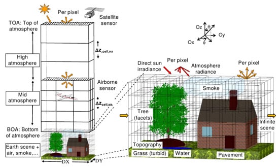
DART is a three-dimensional (3D) model computing radiation propagation through the entire Earth-atmosphere system in the entire optical domain from visible to thermal infrared parts of the electromagnetic spectrum (EMS) [30,31]. As shown in Figure 1, it simulates 3D radiative budget and reflected radiation of urban and natural landscapes as acquired by imaging radiometers and LIDAR scanners aboard of space and airborne platforms. The DART model, developed in the CESBIO Laboratory since 1992, can work with any 3D experimental landscape configuration (atmosphere, terrain geomorphology, forest stands, agricultural crops, angular solar illumination of any day, Earth-atmosphere curvature, etc.) and instrument specifications (spatial and spectral resolutions, sensor viewing directions, platform altitude, etc.). DART forward simulations of vegetation reflectance were successfully verified by real measurements [32] and also cross-compared against a number of independently designed 3D reflectance models (e.g., FLIGHT [26], Sprint [33], Raytran [27]) in the context of the RAdiation transfer Model Intercomparison (RAMI) experiment [34,35,36,37,38]. To date, DART has been successfully employed in various scientific applications, including development of inversion techniques for airborne and satellite reflectance images [39,40], design of satellite sensors (e.g., NASA DESDynl, CNES Pleiades, CNES LIDAR mission project [41]), impact studies of canopy structure on satellite image texture [42] and reflectance [32], modeling of 3D distribution of photosynthesis and primary production rates in vegetation canopies [43], investigation of influence of Norway spruce forest structure and woody elements on canopy reflectance [44], design of a new chlorophyll estimating vegetation index for a conifer forest canopy [45], and studies of tropical forest texture [46,47,48], among others.

Figure 1. DART cell matrix of the Earth/Atmosphere system. The atmosphere has three vertical levels: upper (i.e., just layers), mid (i.e., cells of any size) and lower atmosphere (i.e., same cell size as the land surface). Land surface elements are simulated as the juxtaposition of facets and turbid cells.

Figure 1. DART cell matrix of the Earth/Atmosphere system. The atmosphere has three vertical levels: upper (i.e., just layers), mid (i.e., cells of any size) and lower atmosphere (i.e., same cell size as the land surface). Land surface elements are simulated as the juxtaposition of facets and turbid cells.

DART creates and manages 3D landscapes independently from the RT modeling (e.g., visible and thermal infrared IS, LIDAR, radiative budget). This multi-sensor functionality allows users to simulate several sensors with the sample landscape. Major scene elements are: trees, grass and crop canopies, urban features, and water bodies. A DART simulated tree is made of a trunk, optionally with branches created with solid facets, and crown foliage simulated as a set of turbid cells, with specific vertical and horizontal distributions of leaf volume density. Its crown shape is predefined as ellipsoidal, conical, trapezoidal, or others. Trees of several species with different geometric and optical properties can be exactly or randomly located within the simulated scene of any user-defined size. Grass and crops are simulated as turbid media that can be located anywhere in space. Urban objects (houses, roads, etc.) contain solid walls and a roof built from facets. Finally, water bodies (rivers, lakes, etc.) are simulated as facets of appropriate optical properties. Specific 3D transformations and optical properties can be assigned to each landscape object. 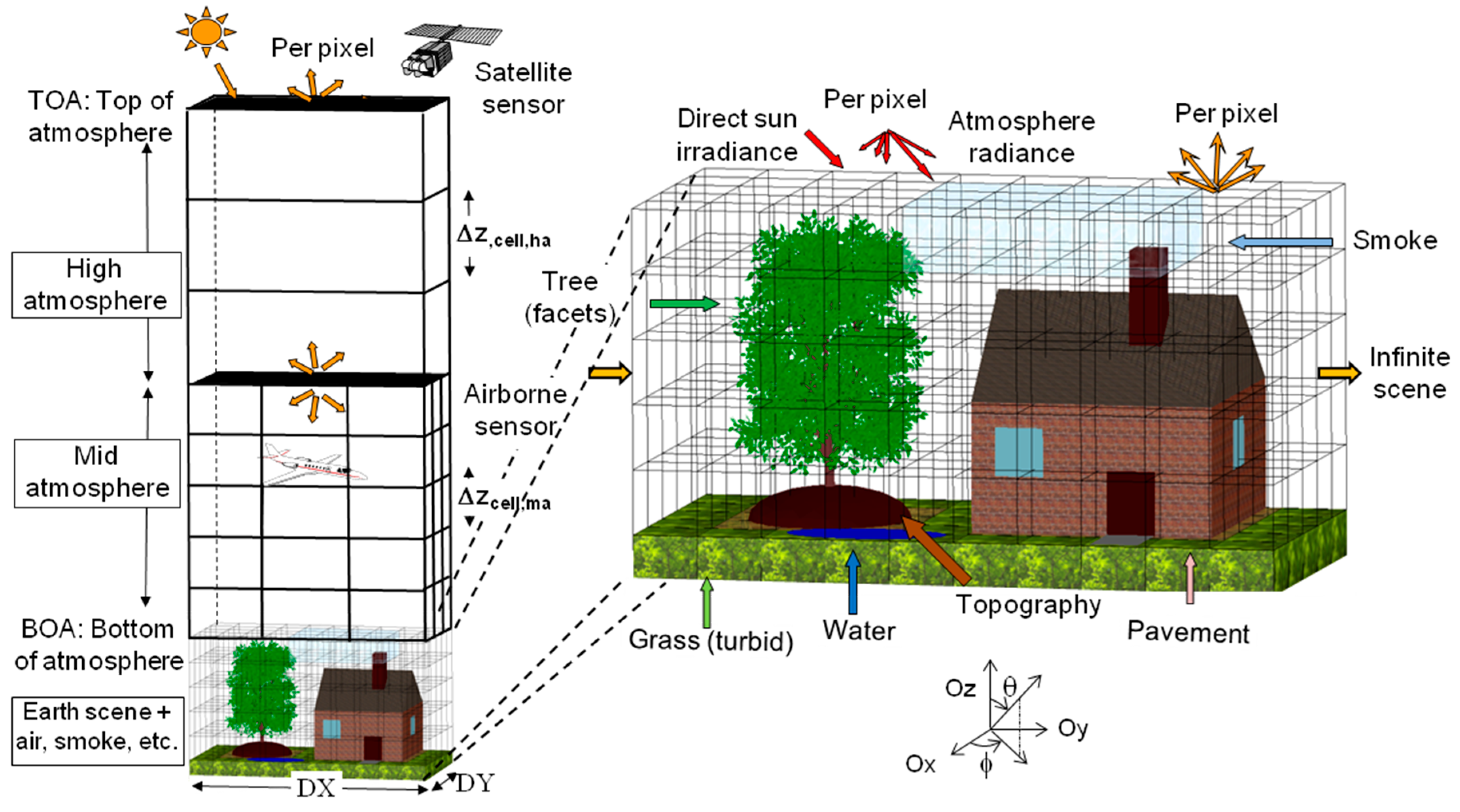Additionally, DART can use external libraries (Figure 2) to import, and to some extent edit (e.g., translation, homothetic and rotation transformations) landscape elements, digital elevation models (DEM) and digital surface models (DSM) produced by other software or measured in field. Importantly, the imported and DART-created landscape objects can be combined to simulate Earth scenes of varying complexity. The optical properties of each landscape element and the geometry and optical properties of the atmosphere are specified and stored in SQL databases.

Figure 2. Examples of natural and artificial 3D objects imported by DART, simulated using triangular facets: (a) wheat plant, (b) corn plant, (c) rice canopy, (d) sunflower plant, (e) cherry tree and (f) airplane.

Figure 2. Examples of natural and artificial 3D objects imported by DART, simulated using triangular facets: (a) wheat plant, (b) corn plant, (c) rice canopy, (d) sunflower plant, (e) cherry tree and (f) airplane.

DART landscapes, hereafter called “scenes”, are constructed with a dual approach as an array of 3D cells (voxels) where each scene element, with any geometry, is created as a set of cells that contains turbid media and/or facets (triangles and parallelograms). Turbid medium is a statistical representation of a matter, such as fluids (air, soot, water, etc.) and vegetation foliage or small-sized woody elements. A fluid turbid medium is a volume of homogeneously distributed particles that are defined by their density (particles/m³), cross section (m²/particle), single scattering albedo, and scattering phase function. Turbid vegetation medium is a volume of leaf elements that are simulated as infinitely small flat surfaces that are defined by their orientation, i.e., Leaf Angle Distribution (LAD; sr⁻¹), volume density (m²/m³), and optical properties of Lambertian and/or specular nature. Finally, a facet is a surface element that is defined by its orientation in space, area and optical properties (Lambertian, Hapke, RPV and other reflectance functions with a specular component, and also isotropic and direct transmittance). It is used to build virtual houses, plant leaves, tree trunks or branches. Vegetation canopies can, therefore, be simulated as assemblies of turbid medium voxels or geometrical primitives built from facets or combination of both.

Atmospheric cells were introduced into DART in order to simulate attenuation effects for satellite at-sensor radiance and also to model the influence of atmosphere on the radiative budget of Earth surfaces. The atmosphere can be treated as an interface above the simulated Earth scene or as a light-propagating medium above and within the simulated Earth scene, with cell sizes inversely proportional with the particle density. These cells are characterized by their gas and aerosols contents and spectral properties (i.e., phase functions, vertical profiles, extinction coefficients, spherical albedo, etc.). These quantities can be predefined manually or taken from an atmospheric database. 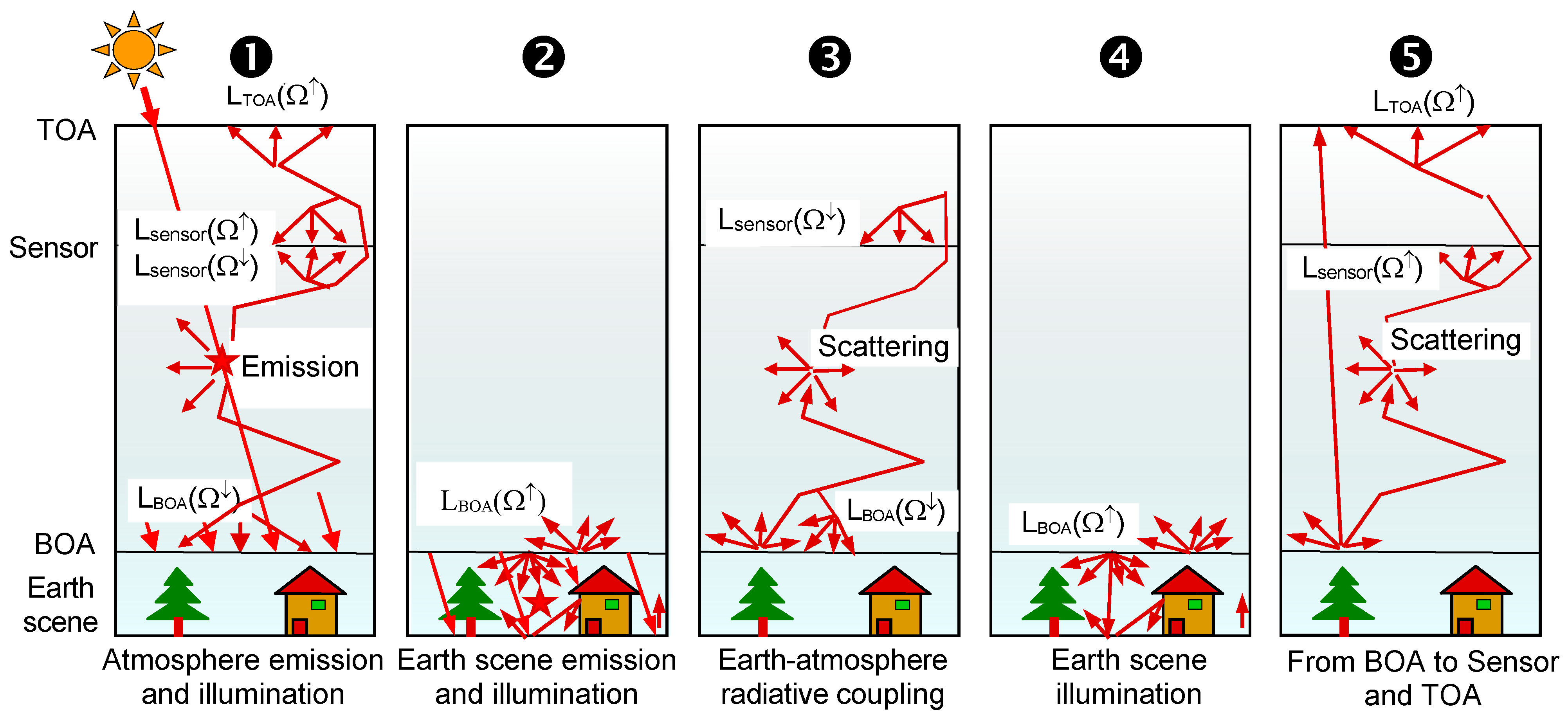DART contains a database that stores the properties of major atmospheric gases and aerosol parameters for wavelengths between 0.3 μm and 50 μm [18]. In addition, external databases can be imported, for instance from the AErosol RObotic NETwork (AERONET) or the European Centre for Medium-Range Weather Forecasts (ECMWF). Atmospheric RT modeling includes the Earth-atmosphere radiative coupling (i.e., radiation that is emitted and/or scattered by the Earth can be backscattered by the atmosphere towards the Earth). It can be simulated for any spectral band within the optical domain from the ultraviolet up to the thermal infrared part of electromagnetic spectrum. The Earth-atmosphere coupling was successfully cross-compared [49,50] with simulations of the MODTRAN atmosphere RT model [18].

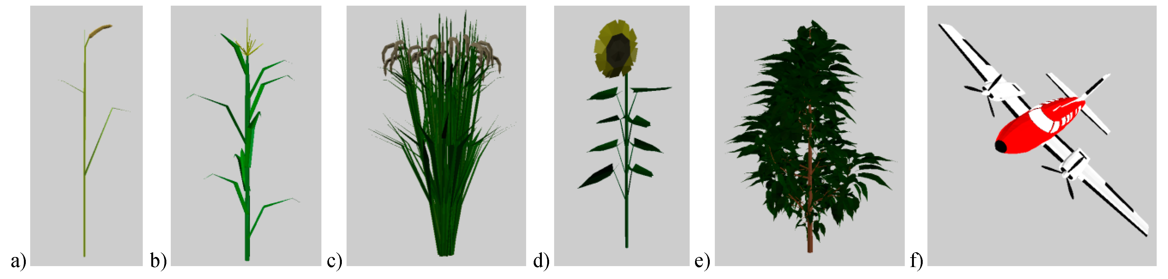
A basic DART simulation procedure is carried out with four processing modules: (i) Direction, (ii) Phase, (iii) Maket, and (iv) Dart (Figure 3). The Direction module computes discrete directions of light propagation with radiation being propagated along N discrete directions Ω_n with an angular sector width ΔΩ_n (sr). Any number of N discrete directions (Ω_n, ΔΩ_n) can be specified with any Ω_n angular distribution and for any ΔΩ_n solid angle range, as for example for oversampling angular regions with an anisotropic radiative behavior such as the hop spot configuration [51]. The discrete directions are calculated automatically or adapted to any user specified configuration. They include a set of U directions that sample the 4π space (${\sum }_{\text{u}=1}^{\text{U}}\Delta {\text{Ω}}_{\text{u}}=4$) and V directions (Ω_v, ΔΩ_v) that are called fictive directions because fluxes along these directions do not contribute to fluxes along any other direction where N = U + V. Importantly, in addition to these discrete directions, DART can also track radiation along any direction in the 4π space, for example for simulating airborne acquisitions and LIDAR signals. These so-called flexible directions are not pre-defined. Their number depends on the number of emitting and scattering elements towards the sensor. Depending on the scene dimensions, the number of flexible directions can exceed 10⁶.

Optical properties for all non-flexible discrete directions are pre-computed with the Phase module. It computes the scattering phase functions of all scene and atmosphere elements depending on their geometry and optical properties. For example, the phase functions of vegetation depend on the actual leaf reflectance and transmittance and the plant specific LAD.

The Maket module builds the spatial arrangement of landscape elements within a simulated scene. Scene features are created and/or imported as 3D objects with specified optical properties. Importantly, scene cell dimensions (Δx, Δy, Δz) define the output spatial sampling, and cell dimensions in DART can be varied within the same scene in order to optimize the final resolution.

Finally, the Dart module computes radiation propagation and interactions for any experimental and instrumental configuration using one of the two computational approaches: (i) Ray tracking and (ii) Ray-Carlo. Ray tracking simulates radiative budget and images of optical airborne and satellite radiometers. For that, it tracks iteratively radiation fluxes W(r, Ω_n) along N discrete directions (Ω_n), and one flexible flux, at any location r [20,21]. These fluxes are defined by three components: their total intensity, the radiation unrelated to leaf biochemistry and the polarization degree associated to first order scattering. The values of these components depend on thermal emission and/or scattering, which in turn depend on local temperature and optical properties of intercepted surfaces or volumetric scattering elements. A scattering event at iteration i gives rise to N fluxes, and the event is repeated in latter iterations. The fraction of W(r, Ω_i) that is scattered along a given Ω_j direction is defined by the local scattering phase function P(Ω_i →Ω_j), with Ω_i being a non-fictive discrete direction, or a set of discrete directions, and Ω_j being a direction that can be discrete, fictive and flexible.

The second modeling approach simulates terrestrial, airborne, and satellite LIDAR signals from waveforms and photon counting RS instruments. It combines two methods that are described in the LIDAR section. Using Monte Carlo and ray tracking techniques [52,53,54], the Ray-Carlo method tracks radiometric quantities corresponding to photons with specific weights, which are for simplicity reasons called just photons. During a scattering event, the so-called Box method determines the discrete direction of photon scattering using the same scattering functions as the Ray tracking approach. Simultaneously a photon with a very small weight is tracked to the LIDAR sensor. Ray tracking can additionally simulate solar noise that is present in a LIDAR signal.

Figure 3. Scheme illustrating DART model architecture: four processing modules (Direction, Phase, Maket, Dart) and input data (landscape, sensor, atmosphere) are controlled through a GUI or pre-programmed scripts. The Sequence module can launch multiple DART simulations simultaneously on multiple processor cores producing effectively several RT products.

Figure 3. Scheme illustrating DART model architecture: four processing modules (Direction, Phase, Maket, Dart) and input data (landscape, sensor, atmosphere) are controlled through a GUI or pre-programmed scripts. The Sequence module can launch multiple DART simulations simultaneously on multiple processor cores producing effectively several RT products.

Apart from the four basic modules, the following supportive tools are integrated in DART distribution to facilitate quick and easy simulations and subsequent analysis of simulated results:

-

Calculation of foliar reflectance and transmittance properties with the PROSPECT leaf RT model [16], using leaf biochemical properties (i.e., total chlorophyll content, carotenoid content, equivalent water thickness and leaf mass per area) and leaf mesophyll structural parameter.

-

Computation of scene spectra and broadband image data (reflectance, temperature brightness, and radiance), using a sensor specific spectral response function for either a single DART simulation with N spectral bands, or for a sequence of N single spectral band simulations.

-

Importation of raster land cover maps for creating 3D landscapes that contain land cover units, possibly with 3D turbid media as vegetation or fluid (air pollution, low altitude cloud cover, etc.).

-

Importation or creation of Digital Elevation Models (DEM). DEMs can be created as a raster re-sampled to the DART spatial resolution or imported either from external raster image file or as a triangulated irregular network (TIN) object.

-

Automatic initiation of a sequence of Q simulations with the Sequence module. Any parameter (LAI, spectral band, date, etc.) A₁, …, A_m can take N₁, …, N_m values, respectively, with any variable grouping ($\text{Q}\le \prod _{\text{i}=1}^{\text{M}}{\text{N}}_{\text{i}}$). Outcomes are stored in a Look-Up Table (LUT) database for further display and analysis. It is worth noting that a single ray tracking simulation with N bands is much faster than the corresponding N mono-band simulations (e.g., 50 times faster if N > 10³).

-

The simulated 3D radiative budget can be extracted and displayed over any modeled 3D object and also as images of vertical and horizontal layers of a given 3D scene.

-

The transformation from facets to turbid medium objects converts 3D plant objects (trees) composed of many facets (> 10⁶) into a turbid vegetation medium that keeps the original 3D foliage density and LAD distribution. This method remediates constraints limiting RT simulations with many vegetation objects (e.g., forest) that lead to too large computational times and computer memory requirements.

-

The creation of 3D objects by using volumes with pre-defined shapes that can be filled with various 3D objects (triangles, discs, etc.). This functionality allows a quick test of simple hypotheses, as for instance the influence of vegetation leaf shape and size in turbid media simulations.

-

The transformation of LIDAR multi-pulse outputs into industrial Sorted Pulse Data (SPD) format [55]. Implementation of the SPDlib software allows users to create, display, and analyze their own LIDAR point clouds [56].

-

Display tools for visualization and quick analysis of spectral images and LIDAR waveform and photon counting outputs, etc.

While the basic DART modules are programmed in C++ language (~400,000 lines of code), most external tools are written in Python language. In addition, a Graphic User Interface (GUI), programmed in Java language, allows users to manage model inputs (RT approach, scene geometry, view direction, etc.), to specify required output products (BRF, radiative budget, etc.), display results, and run the external scripts. A strong feature of DART is acceleration of RT modeling using multithreaded computation, allowing use of a specified number of processor cores simultaneously, which results in a near linear scaling of the processing time.

3. Ray Tracking Approach for Modeling Spectroradiometer Acquisitions

Ray tracking in heterogeneous 3D landscapes [20] and atmosphere [50] is based on exact kernel and discrete ordinate methods with an iterative and convergent approach. Radiation intercepted by scene elements at iteration i is scattered during the following iteration i + 1. The iterative process stops when the relative difference in scene exitance between two consecutive iterations is less than a specified threshold. In addition, any ray is discontinued if its angular power ($\text{W}\cdot {\text{sr}}^{-1}$) is smaller than the scene mean angular power that is scattered at first iteration, multiplied by a user specified coefficient.

The ray tracking approach has three simulation modes: reflectance (R), temperature (T), and combined (R + T). The R mode allows simulating the shortwave optical domain using the sun as the primary source of radiation and the atmosphere as the secondary source. Landscape and atmosphere thermal emissions are neglected. The opposite is true in the (T) mode, where the solar radiation is neglected. Finally, all radiation sources are combined in (R + T) mode, which is particularly useful for simulating RS signals in the spectral domain of 3–4 µm. Dependence of thermal emission on temperature and wavelength is modeled with Planck’s law, while the Boltzmann’s law can be used when simulating radiation budget over the whole electromagnetic spectrum.

The finite DART simulation can be conducted over three landscape arrangements: an infinite repetitive landscape with repetitive topography, an infinite repetitive landscape with continuous topography, and a spatially isolated scene, each of them managing exiting rays differently. A ray {A - A₁} that exits the flat infinite repetitive scene at point A₁ re-enters the scene through the symmetric point B₁ along the same direction (Figure 4). The path ray {A - A₁ - B₁ - A₂ - B₂ - …- C} is, therefore, equivalent to the path {A - C'}. In a similar fashion, a ray {A - A₁} that exits the infinite repetitive scene with continuous topography at point A₁ re-enters the scene under the same direction through the point B₁, which is vertically shifted by the distance equal to the ground altitude offset between the exit and re-entry sides of the scene. In case of an isolated scene, a ray that exits the scene is dismissed; i.e., it does not re-enter the scene.

Figure 4. Simulation of a flat infinite repetitive landscape.

Figure 4. Simulation of a flat infinite repetitive landscape.

The Earth-atmosphere RT is simulated in five consecutive stages (Figure 5) [50]:

-

Stage 1 is tracking the sun radiation and the atmosphere thermal emission through the atmosphere. It calculates radiance transfer functions per cell and per discrete direction from the mid/high atmosphere interlayer to the sensor, TOA and BOA levels. This stage gives the downward BOA radiance L_boa(Ω^↓), upward TOA radiance L_toa(Ω^↑) and also upward L_sensor(Ω^↑) and downward L_sensor(Ω^↓) radiance at sensor altitude.

-

Stage 2 is tracking within the landscape the downward BOA radiance L_boa(Ω^↓), originating from the stage 1, and the landscape thermal emission. This stage provides the landscape radiation budget, albedo, and upward BOA radiance L_boa(Ω^↑), before the Earth-atmosphere radiative coupling.

-

Stage 3 is tracking the BOA upward radiance L_boa(Ω^↑), obtained during stage 2, through the atmosphere back to the landscape. Radiance transfer functions of stage 3 provide the downward BOA radiance L_boa(Ω^↓), which is extrapolated in order to consider the multiple successive Earth-atmosphere interactions.

-

Stage 4 is tracking downward BOA radiance L_boa(Ω^↓), resulting from stage 3, within the landscape. It uses a single iteration with an extrapolation for considering all scattering orders within the Earth scene. This stage results in landscape radiation budget and upward BOA radiance L_boa(Ω^↑).

-

Stage 5 applies the stage 3 radiance transfer functions to the upward BOA radiance of stage 4. The resulting radiance is added to the atmosphere radiance, which is calculated within the first stage, to produce the radiance at sensor (L_sensor(Ω^↑)) and TOA (L_toa(Ω^↑)) levels.

The entire RT procedure results in the following two types of products:

(1)

Images at three altitude levels: BOA, TOA and anywhere between BOA and TOA. They can be camera and/or scanner images with projective and/or orthographic projection, as well as ortho-projected images that allow superimposing the landscape map and images simulated for various viewing directions.

(2)

3D radiative budget: distribution of radiation that is intercepted, absorbed, scattered and thermally emitted. It is useful for studying the energy budget and functioning of natural and urban surfaces.

Figure 5. Five stages of the DART algorithm that models RT of the Earth-atmosphere system.

Figure 5. Five stages of the DART algorithm that models RT of the Earth-atmosphere system.

Finally, scattering and emission of a DART cell corresponds to surface and volume interactions. It is modeled using a sub-division of each cell into D³ sub-cells, resulting in six D² cell sub-faces. This approach improves greatly the spatial sampling, resulting in shorter computational time, and requires less computer memory than using cells with a dimension divided by D, which is very beneficial for simulating scenes with dense turbid cells and large scene elements.

3.1. Surface Interactions with Facets

A ray of light incident on a facet (Figure 6a) interacts with its front side but not with its rear side. Thus, depending on the type of object, any surface can be simulated using only top facets or using top and bottom facets with opposite normal vectors, and optionally with different optical properties. Any facet is characterized by a direct transmittance T_dir along its normal direction Ω_n, a Lambertian transmittance T_diff, and a reflectance R with T_diff + R ≤1. R can be isotropic (Lambertian) or anisotropic. Direct transmittance along Ω_s is equal to [T_dir]^{1/|Ω_s.Ω_n|}. For an incident irradiance E along Ωn, scattered exitance is equal to $\text{E}\cdot \left(1-{\text{T}}_{\text{dir}}\right)\cdot \text{R}$ and transmitted diffuse exitance is equal to $\text{E}\cdot \left(1-{\text{T}}_{\text{dir}}\right)\cdot {\text{T}}_{\text{diff}}$.Surface reflectance anisotropy can be described by parametric functions (e.g., Hapke [15], RPV [6]), with a specular component, defined by a surface refraction index, an angular width and a multiplicative factor.

The point M_int that represents light interception by a facet is modeled as a centroid of all interceptions on that facet. It is calculated per DART constructed sub-cell, among the D³ sub-cells, which is improving spatial sampling, particularly if facets have large dimensions compared to cell dimensions. Storing the intercepted radiation for every direction is computationally expensive, especially for large landscapes with many cells. Thus, a simplifying mechanism storing intercepted radiation per ray incident angular sector Ω_sect,k, where Ω_sect,k is a set of neighboring discrete directions that sample the 4π space of directions (Σ_k∙Ω_sect,k = 4π), was adopted [57,58]. Scattering at an iteration i is then computed from energy locally intercepted within incident angular sectors Ω_sect,k at iteration i – 1. Although, one can define as many angular sectors as discrete directions, ten sectors are sufficient to obtain very accurate results, with relative errors smaller than 10⁻³ [30]. Facets belonging to the same cell can intercept rays scattered and emitted by other facets. Rays exiting the cell through the same cell sub-face are grouped per discrete direction (Figure 6b), reducing the number of rays to track and consequently decreasing total computational time.

Facet thermal emission is simulated according to Planck’s or Boltzmann’s law, using the corresponding facet temperature and optical properties [59].

Figure 6. Facet scattering. (a) Single facet with an incident flux W_inc(Ω_s). It produces reflection W_refl(Ω_n) and direct W_trans,dir(Ω_s) and diffuse W_trans,dif(Ω_m) transmission. (b) Interaction of two facets in cell with 27 sub-cells (only nine are illustrated in 2D figure). Each facet has a single scattering point per sub-cell, with an intercepted radiation per incident angular sector.

Figure 6. Facet scattering. (a) Single facet with an incident flux W_inc(Ω_s). It produces reflection W_refl(Ω_n) and direct W_trans,dir(Ω_s) and diffuse W_trans,dif(Ω_m) transmission. (b) Interaction of two facets in cell with 27 sub-cells (only nine are illustrated in 2D figure). Each facet has a single scattering point per sub-cell, with an intercepted radiation per incident angular sector.

3.2. Volume Interactions within Turbid Vegetation and Fluid Cells

When a ray crosses a turbid cell, two interception points M_int are computed along its path within the cell (Figure 7a). The first point is computed for upward scattering and the second one for downward scattering. As several rays cross each cell, possibly through the same sub-face, two simplifying steps are adopted. First, M_int is calculated per incident cell sub-face s, through which the rays entered the cell, in order to improve spatial sampling, particularly in presence of scenes with large cells. Second, similarly to facet interactions, the intercepted radiation is calculated per incident angular sector Ω_sect,k. The first order scattering is computed at each iteration using the intercepted radiation that corresponds to the incident ray that entered the cell through one or several sub-faces. Thus, intercepted vector sources W_int(s, Ω_sect,k) are stored per sub-face s and per incident angular sector Ω_sect,k. Then, we have: W_int(s, Ω_sect,k) = ΣΩ_s∙W_int(s, Ω_s), with Ω_s ⊂ Ω_sect,k. The first order scattering of the direct solar flux can be computed exactly, because the sun direction is considered as a sector. Within cell multiple scattering (Figure 7b) is analytically modeled [20]. Similarly to the case of facets, rays exiting the same cell sub-face in the same direction are grouped together in order to reduce computational time (Figure 7c).

Cell thermal emission is simulated with Planck’s or Boltzmann’s law and a temperature-independent factor that depends on the cell optical properties and directional extinction coefficient. In order to reduce the RT computation time, this factor is pre-computed as a volume integral in a specified spatial sampling, per cell sub-face, discrete direction and type of turbid medium [59].

Figure 7. Turbid cell volume scattering: (a) two 1st order interception points per incident ray with associated first order scattered rays, and their second order interception points (red), (b) analytically computed within-cell second order scattering, and (c) first order interception points, which are grouped per incident angular sector and per cell sub-face crossed by the incident rays. Rays exiting the cell are grouped per exiting cell sub-face and per discrete direction.

Figure 7. Turbid cell volume scattering: (a) two 1st order interception points per incident ray with associated first order scattered rays, and their second order interception points (red), (b) analytically computed within-cell second order scattering, and (c) first order interception points, which are grouped per incident angular sector and per cell sub-face crossed by the incident rays. Rays exiting the cell are grouped per exiting cell sub-face and per discrete direction.

The spatial resolution of DART images is equal to the cell size (Δx, Δy) divided by a user-defined factor η that sets a spatial oversampling. It is applied during the image creation procedure when upward fluxes are stored into an image array with (Δx/η, Δy/η) pixel sizes. These images can be re-sampled to the pixel-size of any RS sensor by a DART module or by any digital image processing software. Their radiometric accuracy is usually better than if being simulated with a cell size equal to the sensor pixel size. Figure 8 shows DART nadir and oblique images of the citrus orchard site simulated within the RAMI IV experiment [38]. The tree crowns were simulated as a juxtaposition of turbid cells that were transformed into turbid medium from original facet based trees. Cell size of 20 cm was small enough to keep a very good description of 3D tree crown architecture. Its combination with η = 2, allows observation of shadows casted by tree trunks and branches. The simulation with facet-based trees gave very similar reflectance values, however they needed longer computation times [58]. DART can also simulate images of urban scenes. As an example, an example of St. Sernin Basilica (Toulouse, France), with urban elements and trees modeled as combination of facets and turbid medium, is shown in Section 5.

Figure 8. DART simulated RGB composite of satellite image in natural colors for a virtual tree formation displayed in: (a) nadir, and (b) oblique view.

Figure 8. DART simulated RGB composite of satellite image in natural colors for a virtual tree formation displayed in: (a) nadir, and (b) oblique view.

The possibility to simulate time series of images acquired by a geostationary satellite was recently introduced into DART in the frame of a Centre National d’Etudes Spatiales (CNES, France) project preparing a future high spatial resolution geostationary satellite. The aim was to design a tool that calculates the time interval, for any date and for any region on the Earth, during which the useful radiance L_u,toa that originates from the Earth surface is reliable, while considering the expected sensor relative accuracy (~3%), sensor signal-to-noise ratio, atmosphere, local topography, etc. L_u,toa is the difference between TOA radiance and radiance L_atm due to the atmosphere only. Four typical African landscapes (grass savannah, tree savannah, tropical forest, desert), with varying parameters such as spatial resolution, signal-to-noise ratio and elevation were considered. Simulations used local atmosphere conditions from the AERONET network and ECMWF database. Three specific DART features were used: (i) RT modeling through a spherical atmosphere, (ii) automatic computation of satellite view direction for each Earth coordinates, and (iii) automatic calculation of sun direction for any date, satellite and scene coordinates, etc. Figure 9 illustrates the capacity of DART to simulate geostationary satellite radiance images above Africa at Latitude 0° N, Longitude 17° E and altitude of 36,000 km. In this example, the Earth surface was simulated as Lambertian, with a bare ground reflectance “brown to dark gravelly loam” obtained from the USDA Soil Conservation spectra library. At 443 nm, L_atm variability is large, especially for regions at sunset and sunrise. This demonstrates that the accuracy of L_u,toa depends on the location, season and atmosphere conditions, with sunrise and sunset being the worst conditions. A typical task during the preparation stage of a future satellite mission is to assess the optimal spatial resolution for studying a given type of landscape. This problem was investigated with the assumption that radiance spatial variability, as represented by radiance standard deviation, is the textural information of interest. Figure 10 shows the hourly variation of the standard deviation of L_u,toa at 665 nm for the desert sandy landscape (barchans dune), with spatial resolution ranging from 1 m up to 100 m, for 21 June 2012. As expected, the spatial variability of L_u,toa decreases as image spatial resolution coarsens, which allows selection of the optimal spatial resolution.

Figure 9. DART simulated BOA (a), atmosphere (b) and TOA (c) radiance (W/m²/sr/µm) at 443 nm, for 6 h 44 m (left), 8 h 44 m (middle) and 10 h 44 m (right) UTC as measured by a geostationary satellite at Latitude 0° N, Longitude 17° E and 36,000 km altitude on 21 June 2012.

Figure 9. DART simulated BOA (a), atmosphere (b) and TOA (c) radiance (W/m²/sr/µm) at 443 nm, for 6 h 44 m (left), 8 h 44 m (middle) and 10 h 44 m (right) UTC as measured by a geostationary satellite at Latitude 0° N, Longitude 17° E and 36,000 km altitude on 21 June 2012.

Figure 10. Spatial variability of the useful radiance L_u,toa of a sandy desert dune (25.5° N, 30.4° E, altitude of 78 m), acquired by a future geostationary satellite (0° N, 17° E, altitude of 36,000 km) at 665 nm on 21 June 2012. (a) DART simulated radiance image of a barchan dune at solar noon. (b) Hourly standard deviation of L_u,toa for spatial resolution from 1 m up to 100 m. Sand reflectance was obtained from the ASTER spectral library.

Figure 10. Spatial variability of the useful radiance L_u,toa of a sandy desert dune (25.5° N, 30.4° E, altitude of 78 m), acquired by a future geostationary satellite (0° N, 17° E, altitude of 36,000 km) at 665 nm on 21 June 2012. (a) DART simulated radiance image of a barchan dune at solar noon. (b) Hourly standard deviation of L_u,toa for spatial resolution from 1 m up to 100 m. Sand reflectance was obtained from the ASTER spectral library.

4. Modeling LIDAR Signal with Ray-Carlo and Box Methods

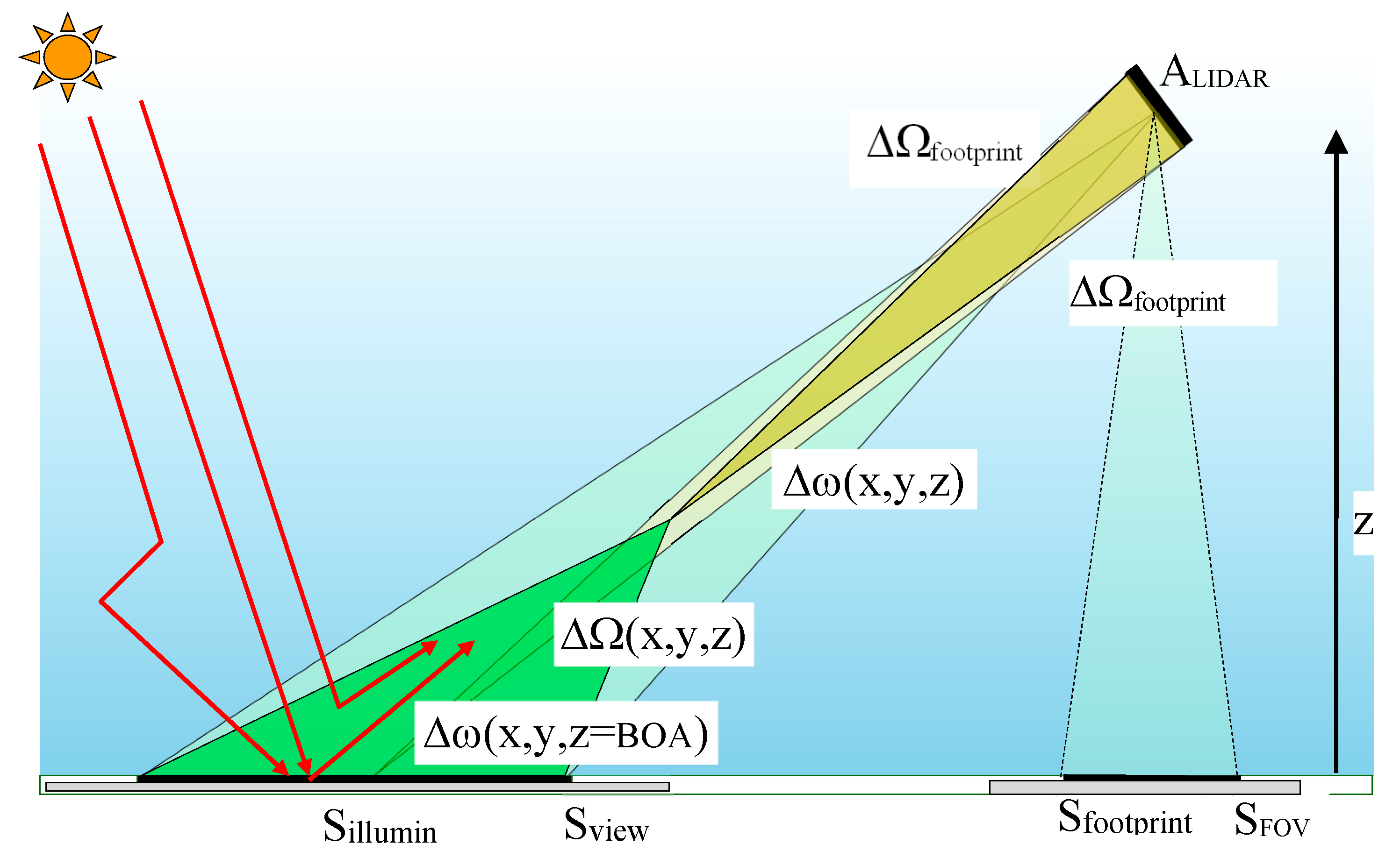
New features related to LIDAR simulations, such as the simulation of airborne LIDAR full-waveform products of single and multiple pulses, as well as LIDAR photon counting and terrestrial LIDAR observations, were recently introduced in DART [53,54]. Figure 11 shows the typical geometry configuration of an airborne laser scanner (ALS). The sensor is defined by a circular footprint with a radius R_footprint defined by the LIDAR illumination solid angle ΔΩ_footprint(α_footprint), the ALS altitude H_lidar and the footprint area ${\text{S}}_{\text{footprint}}=\text{π}\cdot {\text{R}}_{\text{footprint}}^2$. In case of an oblique central illumination direction with a zenith angle θ_l, the 1st order illuminated surface has an elliptical shape with a major axis $\frac{{\text{R}}_{\text{footprint}}}{{\cos }^2{\text{θ}}_{\text{L}}}$, a minor axis $\frac{{\text{R}}_{\text{footprint}}}{\cos {\text{θ}}_{\text{L}}}$, and an area ${\text{S}}_{\text{illumin}}=\frac{{\text{S}}_{\text{footprint}}}{{\cos }^3{\text{θ}}_{\text{L}}}$. Photons launched within ΔΩ_footprint can have any angular distribution (e.g., Gaussian) and pulse characteristics. A photon scattered in the atmosphere at (x,y,z) can illuminate S_illumin within the solid angle ΔΩ (x,y,z). The LIDAR field of view (FOV) is defined either directly as S_fov or by the angle α_fov. The viewed surface covers the area ${\text{S}}_{\text{view}}=\frac{{\text{S}}_{\text{FOV}}}{{\cos }^3{\text{θ}}_{\text{L}}}$. In Figure 11, the ground surface is assumed to be horizontal. However, in presence of terrain topography, the ground altitude is the minimum altitude of provided topography. A photon, which is scattered in atmosphere or landscape at the (x,y,z) position, can irradiate the LIDAR sensor in directions within the solid angle Δω (x,y,z), defined by the sensor aperture area A_lidar.

Figure 11. The LIDAR geometry configuration, with horizontal ground surface.

Figure 11. The LIDAR geometry configuration, with horizontal ground surface.

The Monte Carlo (MC) photon tracing method is frequently used for simulating LIDAR signals [60,61]. It simulates multiple scattering of each photon as a succession of exactly simulated single scattering events, and produces very accurate results. MC can determine if and where photon interception takes place and if an intercepted photon is absorbed or scattered. However, a tiny FOV of LIDAR ΔΩ_fov with an even tinier solid angle Δω (x,y,z), within which the sensor is viewed by scattering events both imply that the probability for a photon to enter the sensor is extremely small. This case, therefore, requires a launch of a tremendous number of photons, which is usually computationally unmanageable. Introduction of anisotropic phase functions into scene elements further increases this number. Consequently, most of the LIDAR simulating RT models use a reverse approach, i.e., they are tracing photons from the sensor instead of from their source [61]. DART, however, uses a different approach for forward simulations of LIDAR signal. Each photon launched from the LIDAR transmission source is tracked within the Earth-atmosphere scene until it is absorbed, measured by sensor or rejected out of the scene. Two modeling methods were devised in order to reduce the computational time constraint: the Ray-Carlo and the Box methods.

4.1. Ray-Carlo: Photon Tracing Method

Any DART volume and/or surface element is characterized by its scattering phase function P(Ω_n → Ω_m). For each photon intercepted by a scene element at (x,y,z) location, the classical MC random pulling uses the element’s single scattering albedo to determine if the photon is scattered, and subsequently what is the discrete direction Ω_m, ΔΩ_m) of the scattered photon. For each scattering event, a particle, called photon for simplicity reasons, is sent to a randomly selected discrete direction (Ω_m, ΔΩ_m) with a weight proportional to the solid angle ΔΩ_m and the phase function P(Ω_n →Ω_m), and another particle is sent directly towards the LIDAR sensor along the direction ω (x,y,z) with a weight proportional to the solid angle Δω (x,y,z) and the phase function P(Ω_n →ω (x,y,z)). The photon along the direction (Ω_m, ΔΩ_m) will contribute to multiple scattering events, conversely to the photon that is sent to the sensor. The latter one has an energy that is negligible compared to the photon scattered along (Ω_m, ΔΩ_m), mostly because Δω (x,y,z) << ΔΩ_m. The photon along Δω (x,y,z) is tracked towards the sensor with an energy (weight) that may decrease, or even become null, as being attenuated by existing landscape and/or atmosphere elements. The energy and the travelled distance are recorded when the photon reaches the sensor. The accumulation of these photons builds up the waveform output, which is used to produce the photon-counting signal via a statistical approach. In practice, scattering of photons sent to the LIDAR is neglected in our modeling approach, because their energy is negligibly small.

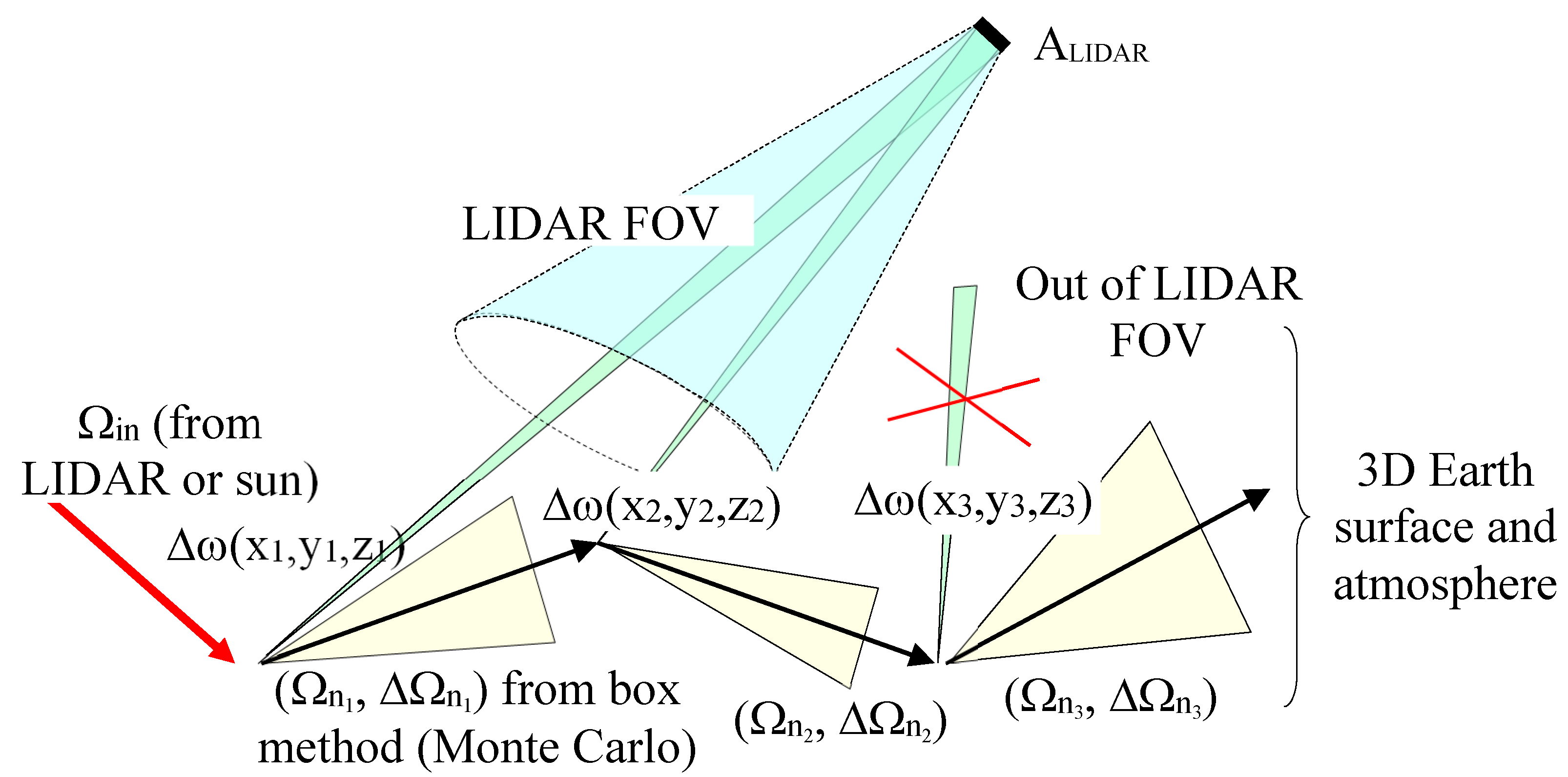
Figure 12 illustrates graphically the DART Ray-Carlo method. A photon of weight w_in, propagated along the direction Ω_in, is intercepted in position (x₁,y₁,z₁). If the MC random pulling provides a positive scattering decision, the photon (weight w_dart,1) is scattered along the DART discrete direction (Ω_n1, ΔΩ_n1) and the position (x₁,y₁,z₁) is verified if the direction towards LIDAR (ω₁) is within ΔΩ_FOV. In case of positive answer, the photon (weight w_lidar,1) is sent towards the LIDAR sensor along the direction ω₁ within the solid angle Δω (x₁,y₁,z₁). The following two equations must be satisfied during this process:

$$w_{in}=w_{LIDAR,1}+w_{DART, 1}$$

(1)

and

$$\frac{w_{LIDAR,1}}{w_{DART,1}}=\frac{{\int }_{\text{Δ}\omega (x_1,y_1,z_1)}P({\text{Ω}}_{in}\to \text{Ω})d\text{Ω}}{{\int }_{{\text{ΔΩ}}_{n1}}P({\text{Ω}}_{in}\to \text{Ω})d\text{Ω}}$$

(2)

For any scattering order i, the direction {ω_i, Δω (x_i,y_i,z_i)} is calculated and the condition within ΔΩ_FOV is checked. It must be noted that ω_i is a flexible direction, independent of the discrete directions. Millions of flexible directions can be simulated, each per a scattering event. For this reason, the phase functions P(Ω_n → ω) of flexible directions cannot be pre-computed as in the case of discrete directions. Thus, P(Ω_n → ω_i) is assumed to be equal to P(Ω_n → Ω_mi), where ω_i lies within the solid angle ΔΩ_mi of a pre-defined discrete direction. It implies that $\frac{{\text{w}}_{\text{LIDAR},1}}{{\text{w}}_{\text{DART},1}}=\frac{{\text{Δω}}_{\text{i}}({\text{x}}_1,{\text{y}}_1,{\text{z}}_1)}{{\text{ΔΩ}}_{\text{mi}}}\approx \frac{{\text{A}}_{\text{LIDAR}}}{{\text{r}}^2\cdot {\text{ΔΩ}}_{\text{mi}}}$, where r is the distance from a scene element to the LIDAR sensor. The photon weight w_lidar,i is, consequently, very small. The GLAS satellite LIDAR [62], with A_lidar ≈ 0.8 m² and r = 6×10⁵ m, has w_lidar,i of around 10⁻¹³. To be able to simulate the acquisition of a single photon with this particular sensor, the use of actual photons without weights would require about 10¹³ scattering events.

Since cells in DART simulated atmosphere are usually bigger than those used for simulating the landscape, a single interception event inside an atmospheric cell that gives rise to a scattering leads to a large uncertainty on the scattering event location defined by the MC random pulling. In order to reduce the associated MC noise without increasing the number of launched photons, K interception events are simulated per interception event along the photon travelling path towards LIDAR FOV. Thus, K photons are sent to the LIDAR, which partially fills the gap of distance recorded based on the random MC pulling with a single scattering event per interception. This approach mimics more closely real behavior of an actual flux of photons, which is continuously intercepted along its path.

Figure 12. The Ray-Carlo approach for LIDAR simulation, depicted with all several scattering orders.

Figure 12. The Ray-Carlo approach for LIDAR simulation, depicted with all several scattering orders.

RT models usually consider the atmosphere as a superimposition of atmospheric layers, each of them being characterized by specific gas and aerosol optical depths. Each layer is defined by constant gas and aerosol extinction coefficients, resulting in a discontinuity of the extinction coefficients at each layer interface. Unlike in case of passive radiometer images, this characterization of the atmosphere leads to inaccurate simulations of LIDAR signals, producing waveforms with discontinuities at the top and bottom of each atmosphere layer. This problem is solved in DART by simulating the atmosphere with vertically continuous gas and aerosol extinction coefficients.

4.2. Box Method: Selection of Photon Scattering Directions

Selection of the discrete direction that corresponds to scattering of a photon incident along a given discrete direction using MC approach is a complex task. Ideally, a function should relate any randomly selected number to a defined discrete direction, and needs to operate between two mathematical spaces: (1) the positive real numbers within [0,1] and (2) the N discrete directions, so that any number within [0,1] corresponds to a unique direction. This means that a bijection map has to be built to link the set of N directions with the corresponding set of N intervals defining the [0,1] interval.

The probability to select the direction j is defined as:

$$\text{𝒫(j)}=\frac{{\int }_{{\text{ΔΩ}}_{\text{i}}}\text{P}({\text{Ω}}_{\text{s}},{\text{Ω}}_{\text{j}}){\text{dΩ}}_{\text{j}}}{{\sum }_{\text{k}=1}^{\text{N}}{\int }_{{\text{ΔΩ}}_{\text{k}}}\text{P}({\text{Ω}}_{\text{s}},{\text{Ω}}_{\text{k}}).{\text{dΩ}}_{\text{k}}}$$

(3)

with $\sum _{\text{j}=1}^{\text{N}}\text{ 𝒫(j)}=1$.

A direct method to determine the direction j is to compare a randomly pulled number with each interval representing each direction. This requires performing a maximum of N comparisons per pulling, which is computationally expensive. This problem can be easily solved if the cumulative probability $𝒫$_cum(n) = $\sum _{\text{j}=1}^{\text{N}}\text{ .𝒫(j)}$ is invertible. Then, random pulling a ∈ [0, 1] gives directly the direction index n = $𝒫$ ⁻¹(a), which indicates the selected direction. However, $𝒫$_cum(n) is, in most cases, not invertible. Several inversion methods (e.g., bisection) were tested, but all of them led to large errors, at least for some directions. Therefore, we developed a Box method that can select the scattering direction rapidly with only two random numbers and without any computation of inverse function.

The Box method keeps in memory an array of boxes, where each box represents a tiny interval of $𝒫$_cum(n) that corresponds to a given direction index (i.e., scattering direction). Subsequently, reading of an array $ℬ$ with a randomly selected number within [0, 1] provides directly a direction index without any need for further computation. The total number of boxes in $ℬ$ is ruled by the user-defined size of computer memory used for its storage. A larger memory size implies that more boxes with smaller probability intervals per box can be stored, giving a better accuracy at each random pulling. The number of lines of $ℬ$ is equal to the N number of incident discrete directions Ω_i and the computer memory is distributed to store the boxes per line of $ℬ$. A various number of boxes per possible scattering direction Ω_j,i is assigned to a single line i of $ℬ$, which is proportional to the probability of occurrence p_j,i = $𝒫$(j|i) of scattering towards the direction j for an incident direction i. The value of each box associated to a given scattering direction Ω_j,i is the index j of that direction. For each line i of $ℬ$, the least probable scattering direction with probability p_1,i is represented by m_1,i boxes, which defines the number M_j,i of boxes per scattering direction Ω_j,i, with total number of boxes M_i = $\sum _{\text{j}=1}^{\text{N}}$ M_j,i. Consequently, a random number m ∈ [0, M_j] defines the scattering direction index. This approach may require quite a large amount of computer memory if the scattering directions have a wide range of occurrence probabilities. For instance, if 10 boxes are used for a scattering direction with a probability of 5×10⁻⁷, then 4×10⁶ boxes are needed for a scattering direction with a probability of 0.2.

The requirement of large computer memory and computation time is solved as follows. Scattering directions Ω_j,i are sorted per incident direction Ω_i according to their occurrence probability. Then, sorted adjacent directions are grouped into classes in such a way that the ratio between maximum and minimum probability over all scattering directions Ω_j,i within the same class is smaller than a given threshold γ. Probability ${\text{P}}_{\text{i}}^{\text{k}}$ of a class k is the sum of occurrence probabilities ${\text{P}}_{\text{j},\text{i}}^{\text{k}}$ of all scattering directions ${\text{Ω}}_{\text{j},\text{i}}^{\text{k}}$, in class k, i.e., ${\text{P}}_{\text{i}}^{\text{k}}=\sum _{\text{j}}{\text{P}}_{\text{j},\text{i}}^{\text{k}}$. Each class k is represented by a number of boxes that depends directly on its probability of occurrence ${\text{P}}_{\text{i}}^{\text{k}}$ for any incident direction Ωi, and a given number of boxes that is assigned to the class with the lower probability. Since two probability arrays are being used, two successive random pulling values are needed for any scattering event with incident direction Ω_i. The first pulling derives the class index k from {${\text{P}}_{\text{i}}^{\text{k}}$}, while the second one derives the direction index j from {${\text{P}}_{\text{j},\text{i}}^{\text{k}}$}. Finally, the value of γ is optimized such a way that probability arrays {${\text{P}}_{\text{i}}^{\text{k}}$} and {${\text{P}}_{\text{j},\text{i}}^{\text{k}}$} require a computer memory smaller than the user specified value. Indeed, if γ is increased, the size of {${\text{P}}_{\text{i}}^{\text{k}}$} decreases with the number of classes, whereas the size of {${\text{P}}_{\text{j},\text{i}}^{\text{k}}$} increases with the number of directions per class.

Figure 13. A virtual tree built out of geometrical facets (a) and the same turbid-cell tree derived by the facet-to-turbid conversion tool (b) with their 3D LIDAR point clouds for an oblique view (θ = 30°, φ= 135°) and the 1D waveform with its first scattering order contribution (c). The image of photons that reached the ground is showing the last LIDAR echo (d) and DART ray tracking provides a high spatial resolution (10 cm) nadir image at λ = 1064 nm.

Figure 13. A virtual tree built out of geometrical facets (a) and the same turbid-cell tree derived by the facet-to-turbid conversion tool (b) with their 3D LIDAR point clouds for an oblique view (θ = 30°, φ= 135°) and the 1D waveform with its first scattering order contribution (c). The image of photons that reached the ground is showing the last LIDAR echo (d) and DART ray tracking provides a high spatial resolution (10 cm) nadir image at λ = 1064 nm.

DART simulations of LIDAR point clouds can be conducted using Ray-Carlo and Box methods for landscapes created with geometrical primitives (facets) and voxels filled with turbid medium. An example of airborne LIDAR sensor viewing a facet based tree created by the AMAP Research Centre under an oblique direction (θ = 30°) at wavelength λ= 1064 nm is presented in Figure 13. High similarity of the two 3D points clouds (i.e., LIDAR echoes) for the two representations, i.e., tree built from facets and transformed into voxels with turbid medium (Figure 13a,b) proves the correct functionality of this timesaving “facet to turbid medium” conversion. 1D waveforms (Figure 13c) display distances measured as time differences between transmission and reception of LIDAR photons. The waveform curve corresponding to multiple scattering orders is significantly larger than the first scattering order curve, which demonstrates high importance of multiple scattering at λ = 1064 nm. It also shows a strong contribution of the ground surface to the simulated signal. Figure 13d shows 2D distribution of photons that reached the ground (i.e., the last echo). As expected, the number of photons tends to be smaller under the tree, relative to the rest of the LIDAR footprint. 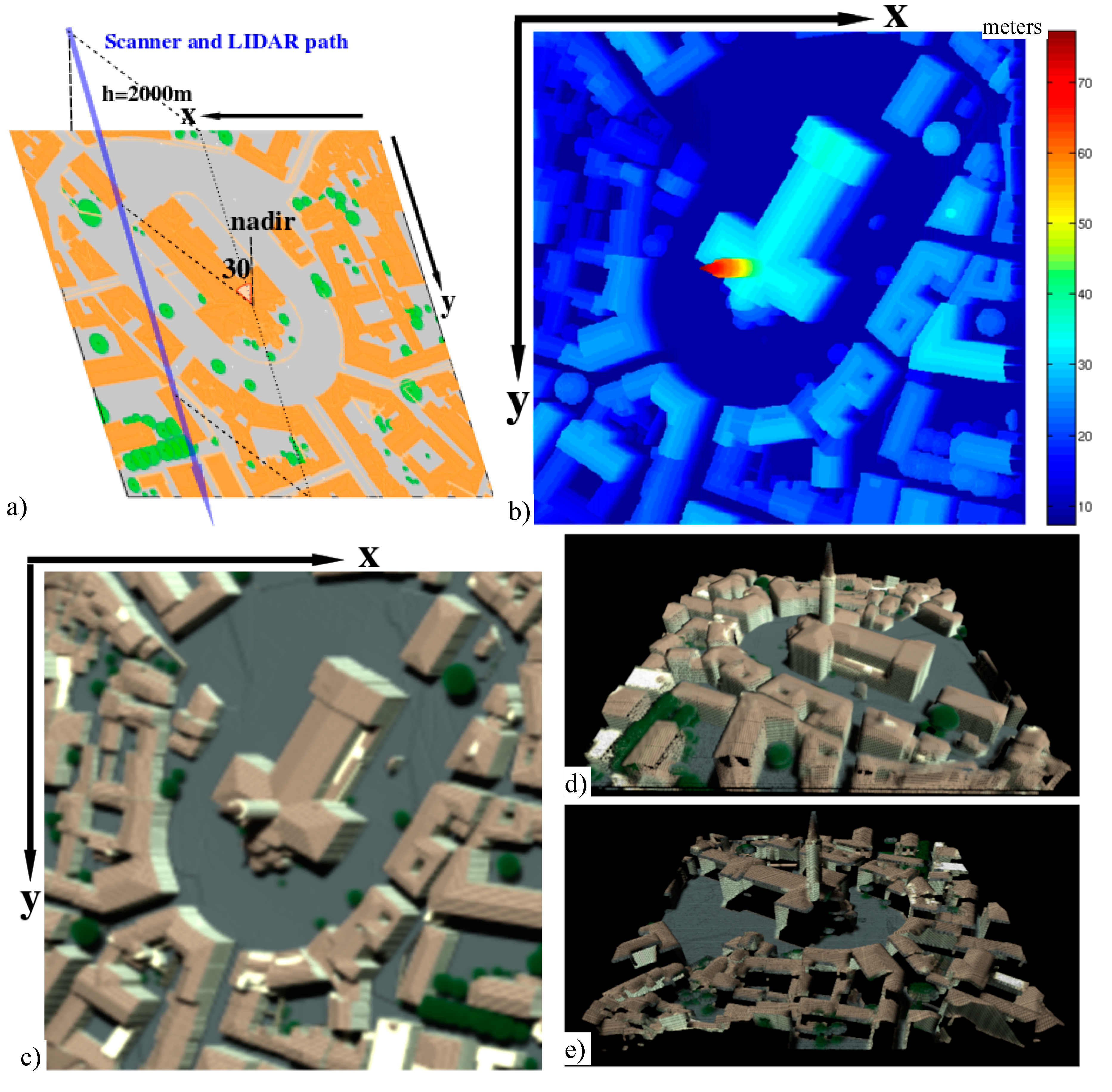Finally, Figure 13e presents image of the simulated facet tree as captured by a nadir imaging spectroradiometer at λ = 1064 nm. The 10 cm spatial resolution provides enough details to detect single leaves. It must be mentioned that in addition to mono-pulse LIDAR, DART can also simulate multi-pulse LIDAR acquisitions for any spectral wavelengths, using a multi-threading algorithm. Such a simulation of the St. Sernin Basilica (Toulouse, France) is shown in Section 5.

Two other LIDAR techniques were implemented in DART, in addition to the airborne/satellite laser scanning: (i) terrestrial LIDAR (TLIDAR), and (ii) photon counting LIDAR. TLIDAR, such as ILRIS-LR can map objects on the ground, resulting in accuracy within millimeters or centimeters. It is increasingly used to assess tree architecture and to extract metrics of forest canopies [63]. TLIDAR simulation within DART is aiming at better understanding of actual data. The photon counting LIDAR is more efficient than conventional LIDAR because it requires only a single detected photon to perform a range measurement. That is why the next ICESat-2 mission [64] will carry a photon counting instrument called the Advanced Topographic Laser Altimeter System (ATLAS). DART simulates photon counting data using the statistical information derived from one or several simulated waveforms. 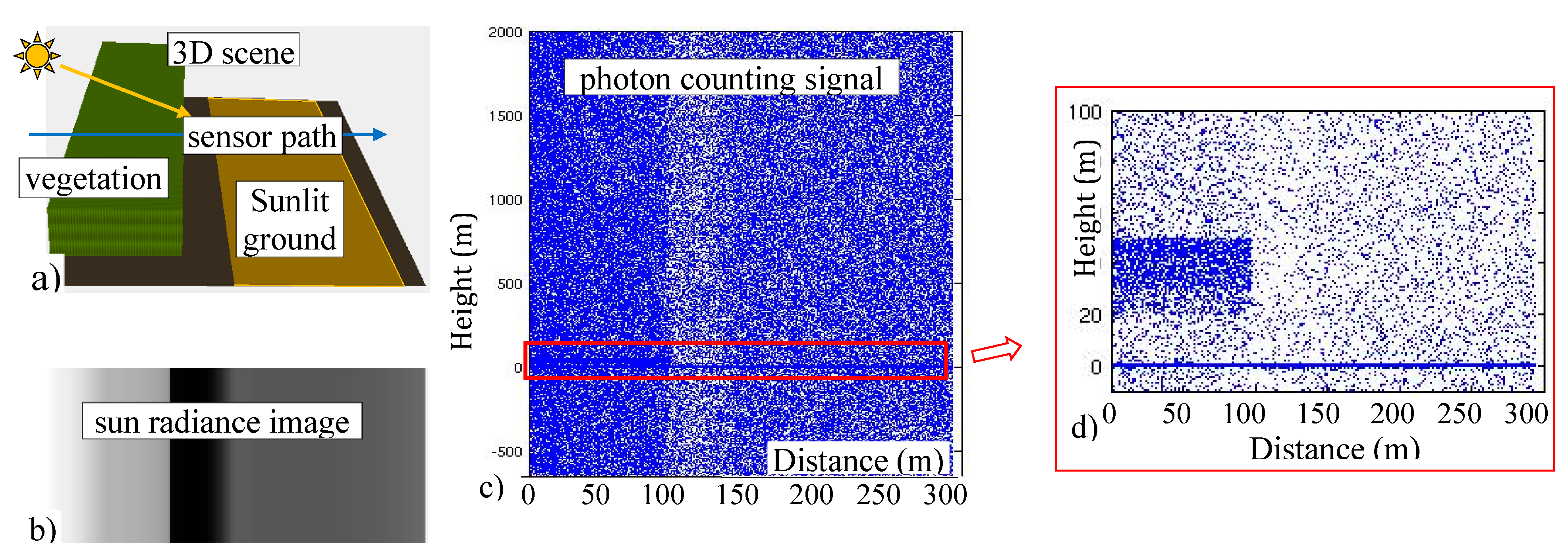Figure 14 shows an example using a simple bare ground with a vegetation plot and signal of a photon counting LIDAR acquired at λ = 1064 nm along a horizontal sensor path, perpendicular to the vegetation plot. Because, the sun direction was set as oblique (θ_s = 45°), part of the bare ground is in the shade of the vegetation cover. Figure 14b shows the radiance image demonstrating the sun illumination, which is used to compute the solar noise of LIDAR signals. Figure 14c illustrates the photon counting simulation along the sensor path (horizontal axis) and Figure 14d is a subset enlargement of Figure 14c. The continuous point cloud above and below the bare ground level corresponds to the solar noise caused by the sun radiation reflected from the bare ground and the vegetation plot. Solar noise is reaching its maxima at the location of the vegetation plot, because vegetation is more reflective than bare ground at 1064 nm. Similarly, solar noise tends to be minimal in the shaded part of the bare ground, where the sun irradiance is diffuse, and consequently minimal.

Figure 14. DART simulated photon counting LIDAR with solar noise. (a) Bare ground and vegetation plot with an oblique sun irradiation (θ_s = 45°) and a horizontal LIDAR sensor path. (b) Radiance image of the scene (i.e., solar noise). (c) Simulated photon counting signal. (d) An enlarged subset of simulated scene (c).

Figure 14. DART simulated photon counting LIDAR with solar noise. (a) Bare ground and vegetation plot with an oblique sun irradiation (θ_s = 45°) and a horizontal LIDAR sensor path. (b) Radiance image of the scene (i.e., solar noise). (c) Simulated photon counting signal. (d) An enlarged subset of simulated scene (c).

5. Modeling IS Data with the Perspective Projection

RT simulations of BRF are usually based on the assumption that the whole landscape is observed along the same viewing direction. This assumption is acceptable when a relatively small landscape is observed from an altitude ensuring that the divergence of the FOV over the landscape can be neglected. However, this disqualifies direct comparison of RT modeled images with actual observations that do not meet this assumption. DART was, therefore, improved to properly consider landscape dimensions together with sensor altitude and consequent sensor FOV [65]. This new functionality provides DART images simulated at large scales with realistic geometries, which allows their per-pixel comparability with actual RS acquisitions. Two types of sensor geometries are available: a pinhole camera and an imaging scanner. Pinhole camera acquisitions are modeled with the perspective projection, where the ray convergence point is unique, whereas imaging scanner acquisitions are modeled with the parallel-perspective projection, where the ray convergent point changes with the platform movement.

The perspective projection is modeled for each sensor pixel (x_s,y_s) located within the sensor focal plane. The pixel value is driven by scattering and/or emission of a facet and/or turbid medium volume at location M(x,y,z) in the horizontal plane $𝒫$z_m. Its associated sensor pixel is viewed from M(x,y,z) along a flexible direction {ω(M), Δω (M)} under zenith angle θ_v, which depends on the location of the scattering point M(x,y,z) and the geometry of sensor pixel S(x_s,y_s,z_s). A scattering and/or emission event at M(x,y,z) gives rise to local fluxes W_n(M) per discrete direction (Ω_n, ΔΩ_n) and to a flexible flux W(ω) that heads towards its associated sensor pixel along the direction {ω(M), Δω(M)}. In order to reduce computational time, the scattering phase function for any flexible direction {ω(M), Δω(M)} is similar to the scattering phase function corresponding with the scattering discrete direction {Ω_n, ΔΩ_n} that contains direction {ω(M), Δω(M)}. Thus, one can write that:

$$\text{W}\left({\text{Ω}}_{\text{s}}\to \text{ω}\right)={\text{W}}_{\text{n}}\left({\text{Ω}}_{\text{s}}\to {\text{Ω}}_{\text{n}}\right).\frac{\text{Δω}\left(\text{M}\right)}{{\text{ΔΩ}}_{\text{n}}},$$

(4)

with

$$\text{ω}\left(\text{M}\right)\subset \{{\text{Ω}}_{\text{n}},{\text{ΔΩ}}_{\text{n}}\}.$$

The upward flux due to the facet scattering at M(x,y,z), which reaches the BOA plane, is computed as:

$${\text{W}}^{\text{*}}\left(\text{M}\right)={\text{T}}_{\text{M}\to \text{BOA}}\left(\text{ω}\right)\times \frac{{\text{W}}_{\text{n}}\left(\text{M}\right)}{{\text{ΔΩ}}_{\text{n}}}.\frac{{\text{S}}_{\text{sensor}}\cdot {\overline{\text{Ω}}}_{\text{sensor}}\cdot \overline{\text{ω}}\left(\text{M}\right)}{{\text{S}}_{\text{scatterer}}\cdot {\overline{\text{Ω}}}_{\text{scatterer}}\cdot \overline{\text{ω}}\left(\text{M}\right)}\times \text{Min}\{\frac{{\text{S}}_{\text{scatterer}}\cdot {\overline{\text{Ω}}}_{\text{scatterer}}\cdot \overline{\text{ω}}\left(\text{M}\right)}{{\text{r}}_{\text{sensor},\text{M}}^2},{\text{ΔΩ}}_{\text{sensor}}\}$$

(5)

with

$${\text{r}}_{\text{sensor},\text{M}}^2={\left({\text{x}}_{\text{s}}-\text{x}\right)}^2+{\left({\text{y}}_{\text{s}}-\text{y}\right)}^2+{\left({\text{z}}_{\text{s}}-\text{z}\right)}^2={\left(\frac{{\text{z}}_{\text{s}}-\text{z}}{\cos {\text{θ}}_{\text{v}}}\right)}^2$$

where ΔΩsensor is the sensor pixel FOV and ${\text{T}}_{\text{M}\to \text{BOA}}(\text{ω})$ is the path transmittance from the scatterer at location M up to the BOA level (top of the Earth scene).

The condition $\text{Min}\{\frac{{\text{S}}_{\text{scatterer}}\cdot {\overline{\text{Ω}}}_{\text{scatterer}}\cdot \overline{\text{ω}}\left(\text{M}\right)}{{\text{r}}_{\text{sensor},\text{M}}^2},{\text{ΔΩ}}_{\text{sensor}}\}$ ensures that the flux, which arrives to a sensor pixel, is not outside ΔΩ_sensor. If ω(M) is within ΔΩ_sensor, we have:

$${\text{W}}^{\text{*}}\left(\text{M}\right)=T_{M\to BOA}(\text{ω}).\frac{{\text{W}}_{\text{n}}\left(\text{M}\right)}{{\text{ΔΩ}}_{\text{n}}}.\frac{{\text{S}}_{\text{sensor}}.{\overline{\text{Ω}}}_{\text{sensor}}.\overline{\text{ω}}(\text{M})}{{\text{r}}_{\text{sensor},\text{M}}^2}$$

(6)

The term 1/r² stresses that a scattered/emitted flux captured within the sensor pixel FOV decreases with the square of the distance from its scattering/emission point. Fluxes that leave an Earth scene are stored in the horizontal plane $𝒫$z_min at the scene minimum altitude z_min. To achieve this, scattering facets and volumes are projected along direction ω(M) into $𝒫$z_min, with M' being the projection of M along ω(M) into $𝒫$z_min, and S_m,xy and S_m',xy being the areas of projections along ω(M) of the scattering element M into $𝒫$z_m and $𝒫$z_min, respectively. Since the projection keeps the radiance constant, one can write:

$$\frac{{\text{W}}^{\text{*}}\left(\text{M}\right)\cdot {\text{r}}_{\text{sensor},\text{M}}^2}{{\text{S}}_{\text{M}}\cdot \cos {\text{θ}}_{\text{v}}\cdot {\text{S}}_{\text{sensor}}\cdot {\overline{\text{Ω}}}_{\text{sensor}}\cdot \overline{\text{ω}}(\text{M})}=\frac{{\text{W}}^{\text{*}}\left(\text{M′}\right)\cdot {\text{r}}_{\text{sensor},\text{M′}}^2}{{\text{S}}_{\text{M′}}\cdot \cos {\text{θ}}_{\text{v}}\cdot {\text{S}}_{\text{sensor}}\cdot {\overline{\text{Ω}}}_{\text{sensor}}\cdot \overline{\text{ω}}(\text{M′})}$$

(7)

It implies that: ${\text{W}}^{\text{*}}\left(\text{M′}\right)={\text{W}}^{\text{*}}\left(\text{M}\right)\times \frac{{\text{Δz}}_{\text{sensor},\text{M}}^2\cdot {\text{S}}_{{\text{M}}^{\text{′}},\text{xy}}}{{\text{Δz}}_{\text{sensor},\text{M′}}^2\cdot {\text{S}}_{\text{M},\text{xy}}}$, with Δz_sensor,m = z_s – z_m and Δz_sensor,m' = z_s – z_m'.

Three sensor projections are considered in DART:

(1)

Orthographic projection with parallel rays to the sensor plane: S_m',xy = S_m,xy, resulting in ${\text{W}}^{\text{*}}\left(\text{M′}\right)={\text{W}}^{\text{*}}\left(\text{M}\right)\times \frac{{\text{Δz}}_{\text{sensor},\text{M}}^2}{{\text{Δz}}_{\text{sensor},{\text{M}}^{\text{′}}}^2}$.

(2)

Perspective projection of a pin-hole camera: ${\text{S}}_{{\text{M}}^{\text{′}},\text{xy}}={\text{S}}_{\text{M},\text{xy}}\times \frac{{\text{Δz}}_{\text{sensor},{\text{M}}^{\text{′}}}^2}{{\text{Δz}}_{\text{sensor},\text{M}}^2}$, resulting in W^*(M') = W^*(M).

(3)

Combined projection of a scanner: orthographic projection for the axis parallel to the sensor path, and perspective for the other axis. Thus, ${\text{S}}_{{\text{M}}^{\text{′}},\text{xy}}={\text{S}}_{\text{M},\text{xy}}\times \frac{{\text{Δz}}_{\text{sensor},{\text{M}}^{\text{′}}}^2}{{\text{Δz}}_{\text{sensor},\text{M}}^2}$ resulting in ${\text{W}}^{\text{*}}\left(\text{M′}\right)={\text{W}}^{\text{*}}\left(\text{M}\right)\times \frac{{\text{Δz}}_{\text{sensor},\text{M}}^{}}{{\text{Δz}}_{\text{sensor},\text{M′}}}$.

During the projection process, W^*(M') and the associated projected surface S_m are spread over DART pixels (Δx, Δy) of $𝒫$z_min. The proportion γ_m'→i,j of W^*(M') in pixel (Δx, Δy) is used to compute the total flux from (Δx, Δy) to the sensor pixel (i,j): ${\text{W}}_{\text{i},\text{j}}^{\text{*}}=\sum _{{\text{M}}^{\text{′}}}{\text{γ}}_{{\text{M}}^{\text{′}}\to \text{i},\text{j}}\times {\text{W}}^{\text{*}}(\text{M′})$, leading to pixel radiance ${\text{L}}_{\text{i},\text{j}}^{\text{*}}=\frac{{\sum }_{{\text{M}}^{\text{′}}}{\text{γ}}_{{\text{M}}^{\text{′}}\to \text{i},\text{j}}\cdot {\text{W}}^{\text{*}}(\text{M′})}{\text{Δx}\cdot \text{Δy}\cdot \cos {\text{θ}}_{\text{v},\text{i},\text{j}}\cdot {\text{Δω}}_{\text{i},\text{j}}}$, where {ω_i,j(θ_v,i,j, φ_v,i,j),Δω_i,j} is the direction under which the sensor is viewed from (i, j). Finally, the sensor image is created by projecting the atmosphere-transmitted radiance onto the sensor plane. Sensor orientation (precession, nutation, and intrinsic angle) is taken into account during this procedure.

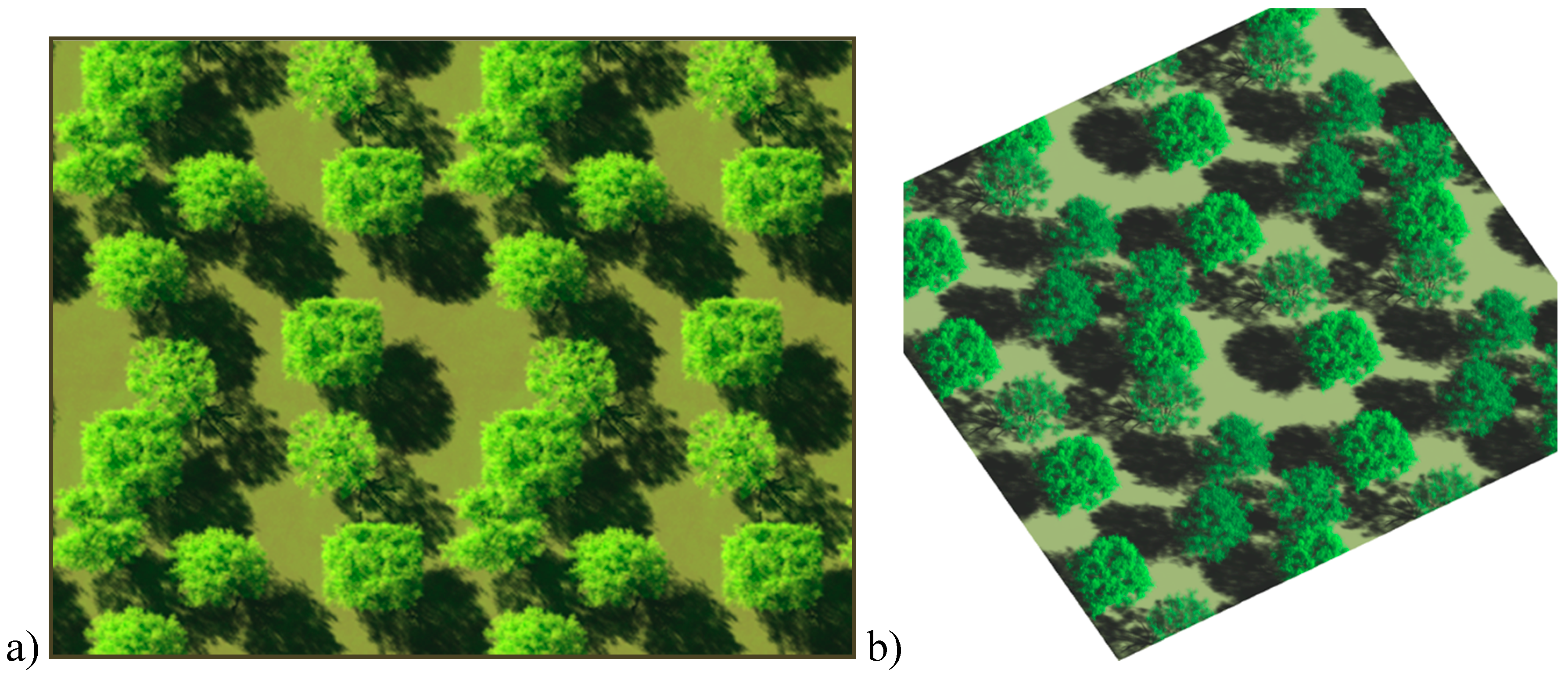
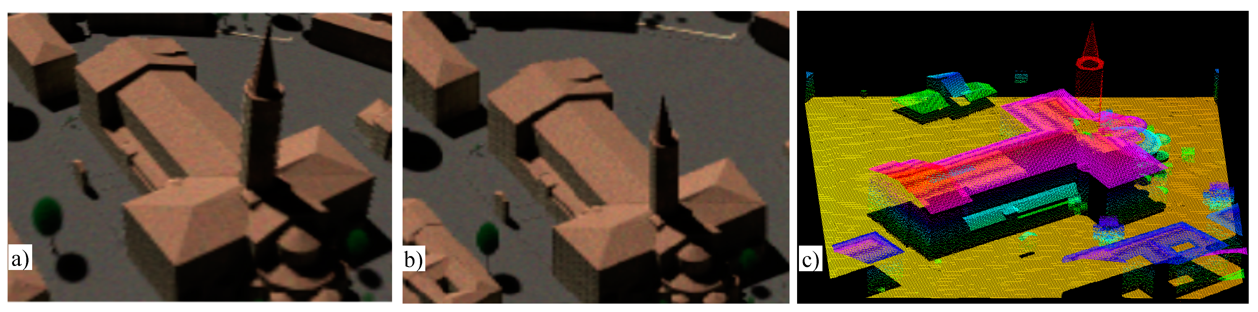
A DART modeled airborne camera image of the St. Sernin Basilica (Toulouse, France) is illustrated in Figure 15a. It differs geometrically from the satellite image simulated with an orthographic projection (Figure 15b). As one can see, two surfaces with the same area and orientation, but located at different places, are having, due to perspective projection, different dimensions in the airborne camera image, but equal dimensions in the orthographic projection of the satellite image. This explains why objects, as for instance the basilica tower and the tree next to it look much larger in the camera image.

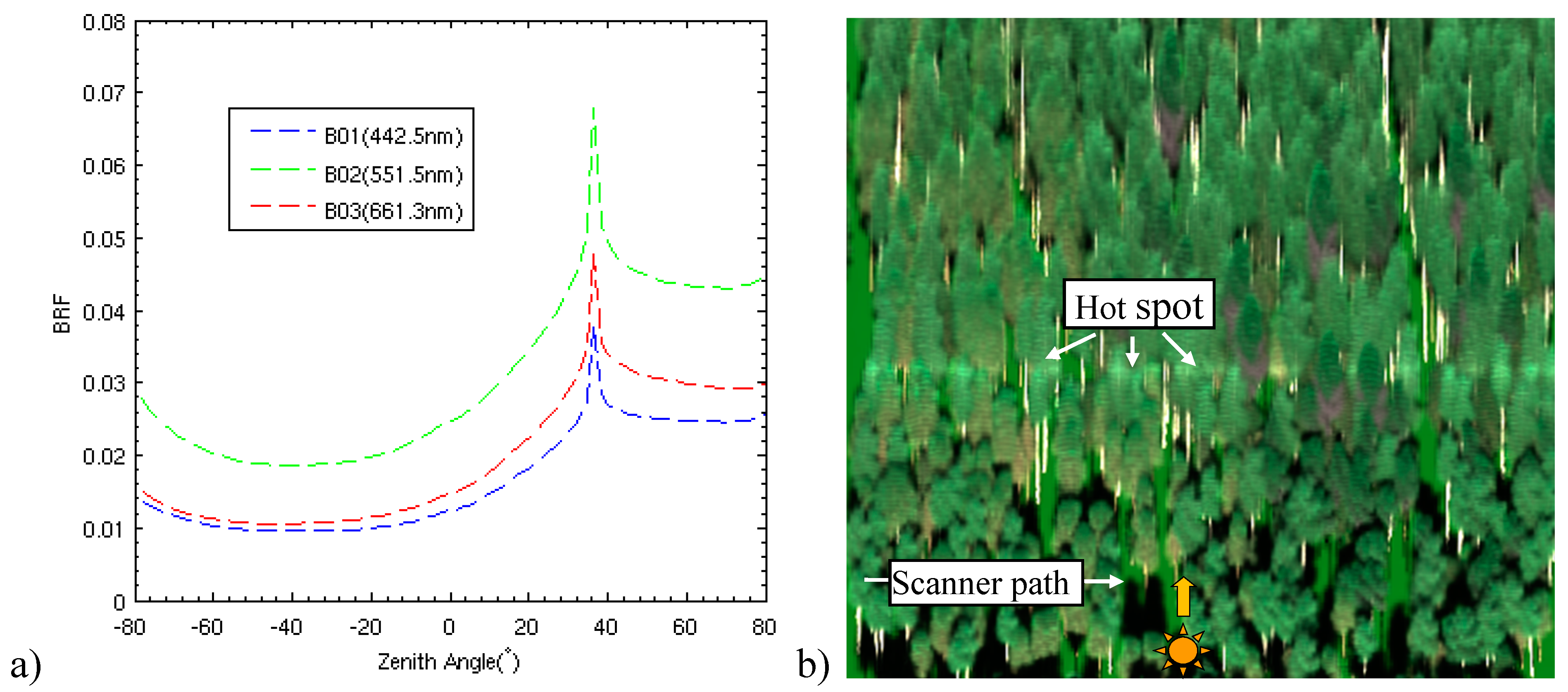
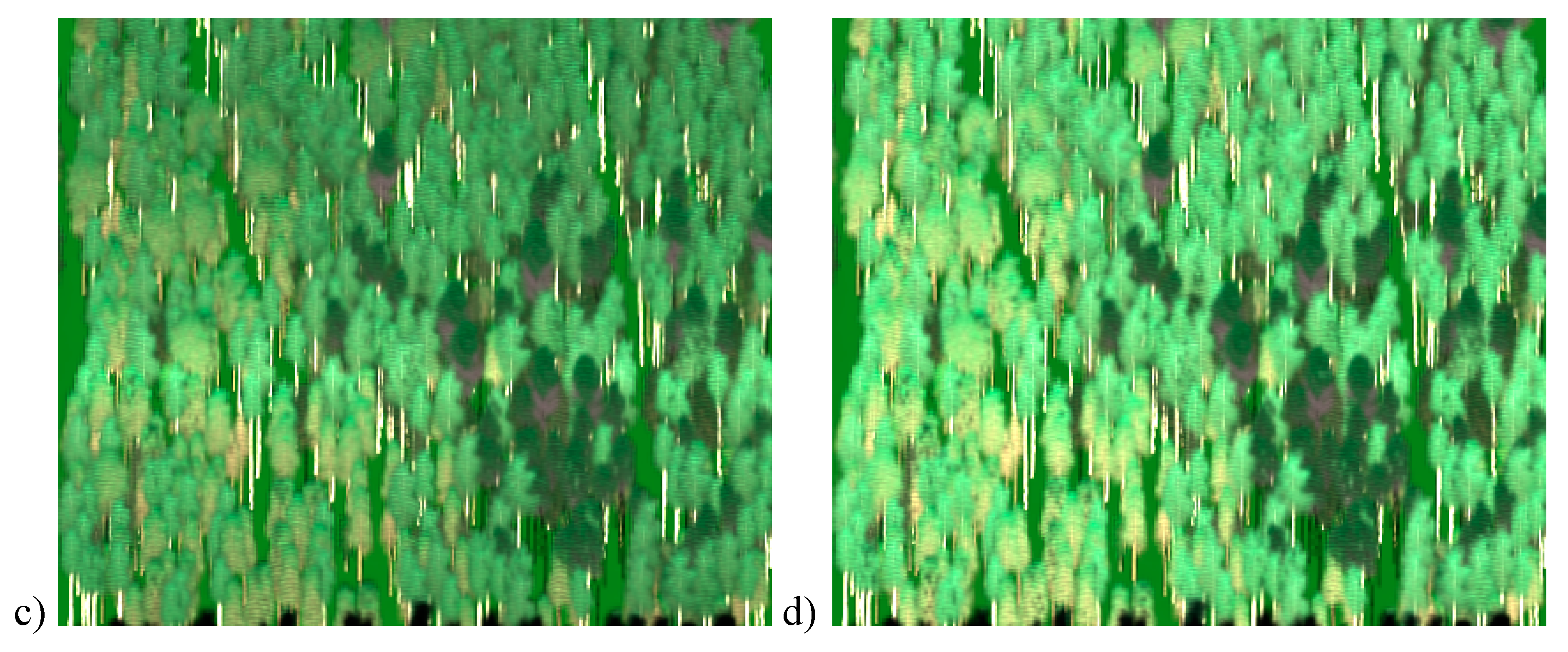
The fact that pixels in a scanner image correspond to different view directions can strongly affect their radiometric values. This is illustrated by DART simulated scanner images of the Jarvselja birch stand (Estonia) in summer (Figure 16). Jarvselja stand is one of the RAMI IV experiment test sites [38]. It is a 103 m × 103 m × 31 m large forest plot, which was simulated as an image with three spectral bands at 442, 551 and 661 nm, with SKYL (fraction of diffuse-to-direct scene irradiance) equal to 0.21, 0.15 and 0.12, respectively. The scanner followed a horizontal path at three flying altitudes of 0.2 km, 2 km and 5 km. The solar zenith angle was 36.6° (in Figure 16, the solar direction goes from the bottom to the top of images), and the ground spatial resolution was equal to 0.5 m for all three acquisitions. For any altitude, the central view direction of the imaging scanner is the hotspot direction. In the hotspot configuration [66], the sun is exactly behind the sensor. As a result, no shadows occur in the sensor’s FOV, providing maximal reflectance values (Figure 16a) represented as a bright horizontal line running parallel to the scanner path of motion (Figure 16b). The hotspot effect (BRF local maximum) is observed in a relatively small angular sector centered in the exact hotspot direction. As expected, the perception of shadows increases rapidly for viewing directions located far from the hotspot direction. At altitude of 0.2 km, the range of the scanner viewing directions over the whole forest scene is relatively large, ranging from 12.3° to 55.4°, and the hotspot phenomenon is therefore visible only along a narrow line. The range of scanner view directions decreases with increasing altitude. It falls between 34.0° and 39.1° at 2 km altitude and between 36.595° and 36.605° at 5 km altitude, which explains why the hotspot line broadens in case of higher observing altitude of 2 km (Figure 16c), and why the whole forest stand is observed under the hotspot configuration at 5 km altitude (Figure 16d).

Figure 15. DART simulated products of the St. Sernin Basilica (Toulouse, France). (a) Airborne camera image (RGB color composite in natural colors) with the projective projection. (b) Satellite image with the orthographic projection. (c) Airborne LIDAR scanner simulation, displayed with SPDlib software.

Figure 15. DART simulated products of the St. Sernin Basilica (Toulouse, France). (a) Airborne camera image (RGB color composite in natural colors) with the projective projection. (b) Satellite image with the orthographic projection. (c) Airborne LIDAR scanner simulation, displayed with SPDlib software.

Figure 16. The changing hotspot perception simulated for the Jarvselja birth forest stand (Estonia) in summer: (a) DART simulated BRF for three spectral bands (442 nm, 551 nm, 661 nm), with SKYL equal to 0.21, 0.15 and 0.12, respectively, and DART simulated images for an airborne scanner flown at three altitudes: (b) 0.2 km, (c) 2 km and (d) 5 km, with ground resolution of 0.5 m. Dark zones in (c) and (d) correspond with occurrences of few pine trees in the birch stand.

Figure 16. The changing hotspot perception simulated for the Jarvselja birth forest stand (Estonia) in summer: (a) DART simulated BRF for three spectral bands (442 nm, 551 nm, 661 nm), with SKYL equal to 0.21, 0.15 and 0.12, respectively, and DART simulated images for an airborne scanner flown at three altitudes: (b) 0.2 km, (c) 2 km and (d) 5 km, with ground resolution of 0.5 m. Dark zones in (c) and (d) correspond with occurrences of few pine trees in the birch stand.

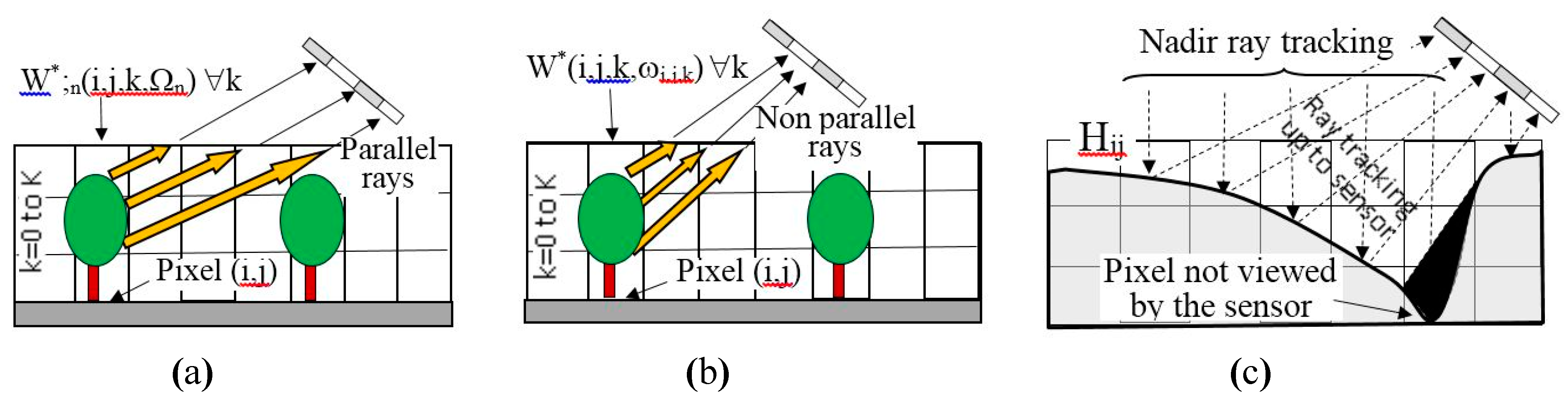
Air-/space-borne RS images are usually transformed into orthorectified products that can be superimposed with local maps. DART computes orthorectified RS images directly, without classical orthorectification methods, because the exact location of each scattering/emission event occurring during an image simulation is known [65]. Two types of orthorectified products are produced by DART (Figure 17): ideally orthorectified images and industry orthorectified images, which are similar to RS images derived by industrial orthorectification methods. In the ideal orthorectification, radiance of pixel (i,j) results from the sum of all the fluxes that originate from scattering events occurring within the voxels (i,j,k) from the bottom up to the top of the scene. Selection of two ideal projections is available in DART:

-

Orthographic projection (Figure 17a): radiance of pixel (i,j) is ${\text{L}}_{\text{i},\text{j}}\left({\text{Ω}}_{\text{n}}\right)=\frac{{\sum }_{\text{k}}^{}{\text{W}}_{\text{n}}^{\text{*}}(\text{i},\text{j},\text{k},{\text{Ω}}_{\text{n}})}{\text{Δx}\cdot \text{Δy}\cdot {\overline{\text{Ω}}}_{\text{g}}\cdot {\overline{\text{Ω}}}_{\text{n}}\cdot {\text{ΔΩ}}_{\text{n}}}$, with ${\overline{\text{Ω}}}_{\text{g}}$ the surface normal vector, (Ω_n, ΔΩ_n) the sensor viewing direction (i.e., DART discrete direction) and k the index of cells above pixel (i,j), and

-

Perspective projection (Figure 17b): radiance of pixel (i, j) is ${\text{L}}_{\text{i},\text{j}}\left({\text{ω}}_{\text{i},\text{j}}\right)=\sum _{\text{k}}\frac{{\text{W}}_{}^{\text{*}}(\text{i},\text{j},\text{k},{\text{ω}}_{\text{i},\text{j},\text{k}})}{\text{Δx}\cdot \text{Δy}\cdot {\overline{\text{Ω}}}_{\text{g}}\cdot {\overline{\text{ω}}}_{\text{i},\text{j}}\cdot {\text{Δω}}_{\text{i},\text{j},\text{k}}}$, with (ω_i,j,k, Δω_i,j,k) being the sensor viewing direction for cell (i,j,k) above pixel (i,j).

The industry orthorectification (Figure 17c), which uses altitude of the Earth surface including any 3D object (e.g., trees, man-made objects, etc.) from a digital surface model (DSM), is carried out in two successive steps. In the first step, nadir downward ray tracking samples the DSM with a spatial sampling equal to that of the created ortho-image. This step provides the altitude H_i,j for each pixel (i, j) of the ortho-image. In the second step, rays are tracked up to the sensor from each H_i,j. Any upward ray originating from H_i,j that is not intercepted within the Earth scene reaches the sensor plane at a point M_sensor. In this case, the sensor radiance value at the point M_sensor is assigned to the pixel (i, j) of the ortho-image. If an upward ray from H_i,j is at least partially intercepted within the Earth scene, then a value of −1 is assigned to the pixel (i,j), which indicates that this pixel cannot be viewed by the sensor (Figure 17c).

Figure 17. Schematic representation of the DART procedure that simulates orthorectified RS images: an ideal orthorectification with orthographic (a) and perspective projection (b), respectively, and an industry orthorectification (c) with either perspective or orthographic projection.

Figure 17. Schematic representation of the DART procedure that simulates orthorectified RS images: an ideal orthorectification with orthographic (a) and perspective projection (b), respectively, and an industry orthorectification (c) with either perspective or orthographic projection.

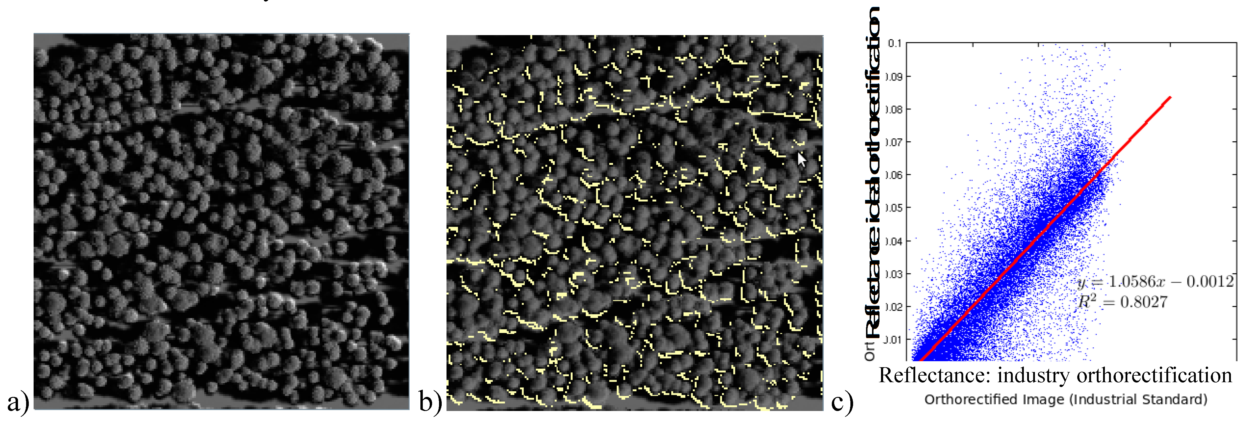
DART ideal orthorectification with orthographic projection, for a satellite optical sensor observing the Jarvselja birch stand with the central viewing zenith angle of 25° and the illumination direction along the horizontal axis, is illustrated in Figure 18a. The same simulation but for industry orthorectification using a DSM that represents the upper surface of the tree canopy is presented in Figure 18b. Bright color tones in Figure 18b indicate deep occlusion areas of the DSM, indicated in Figure 17c, that sensor cannot see due to the 3D nature of forest canopy. No-signal values are assigned to the corresponding pixels. Figure 18c shows scatterplot of reflectance values of both orthorectified images. Although reflectance images are strongly correlated, one can observe numerous outliers originating from different assumptions about the tree canopy surface. It is considered as a non-opaque medium in the ideal orthorectification, but an opaque surface for the industry orthorectification.

Figure 18. DART simulated orthorectified satellite images of the Jarvselja birth forest stand (Estonia) in summer obtained with ideal (a) and industry (b) orthorectification (bright tones indicate zones invisible to the sensor, due to the DSM opacity), accompanied by a scatterplot (c) displaying linear regression between per-pixel reflectance values of both orthorectified images.

Figure 18. DART simulated orthorectified satellite images of the Jarvselja birth forest stand (Estonia) in summer obtained with ideal (a) and industry (b) orthorectification (bright tones indicate zones invisible to the sensor, due to the DSM opacity), accompanied by a scatterplot (c) displaying linear regression between per-pixel reflectance values of both orthorectified images.

6. Fusion of DART Simulated Imaging Spectroscopy and LIDAR Data

New multi-sensor airborne RS systems, such as the Carnegie Airborne Observatory (CAO) [67,68] and the Goddard’s LiDAR, Hyperspectral & Thermal Imager (G-LiHT) [69], are carrying on-board LIDAR and imaging spectrometer instruments simultaneously. The FOV of the instruments are geometrically aligned and both data streams are spatially co-registered. This sensor synergy offers a possibility of an in-flight data fusion, where LIDAR provides structural and geometrical information and imaging spectrometer provides spectral information of observed Earth’s objects. This type of fusion can find its use in various RS applications such as land cover/use classifications, monitoring of natural and man-managed ecosystem services or mapping of vegetation bio-diversity and eco-physiological functions.

Figure 19. DART fusion of LIDAR and spectral images of St Sernin Basilica (Toulouse, France). (a) Acquisition geometry. (b) Multi-pulse LIDAR image. (c) RGB composition of corresponding spectral image. (d) and (e) Products of LIDAR-spectral fusion for two opposite viewing directions.

Figure 19. DART fusion of LIDAR and spectral images of St Sernin Basilica (Toulouse, France). (a) Acquisition geometry. (b) Multi-pulse LIDAR image. (c) RGB composition of corresponding spectral image. (d) and (e) Products of LIDAR-spectral fusion for two opposite viewing directions.

Since DART can apply the ray tracking method to simulate IS and the Ray-Carlo method to simulate LIDAR multi-pulse waveforms of the same landscape in a single run, it can also directly facilitate the in-flight fusion of both simulated datasets. During the first step of this procedure, the position of the LIDAR FOV center at the minimum altitude is recorded per pulse together with corresponding pulse identification number (ID). Then, the imaging scanner image at the minimum altitude is simulated with the parallel-perspective projection. This image is automatically referenced in DART scene coordinate system, which allows the radiance value to be computed in accordance with the FOV center of each recorded LIDAR pulse through a cubic-spline interpolation of the scanner image. The LIDAR output is then converted into the SPD format and processed with the SPDlib software to produce the LIDAR point clouds. Each LIDAR pulse contains n returns, which create n discrete points in 3D space. These points are linked with radiance value via pulse ID, which results in structural information and spectral information of the simulated landscape objects being achieved through the same path of a given pulse.

The DART in-flight data fusion for the St. Sernin Basilica (Toulouse, France) is illustrated in Figure 19. Figure 19a shows the geometrical configuration of the 250 m × 250 m scene with the x and y axes of the DART coordinate system. The aircraft equipped with a LIDAR sensor (λ = 1064 nm) and an imaging spectrometer (three spectral bands at 450 nm: B, 550 m: G, 650 nm: R) was flown at altitude of 2000 m along the y axis, with an off-nadir viewing angle of 30 degrees from the center of the scene to the left side of the flight path. This set up ensures that the walls of buildings in the scene, which are facing positive values of the x-axis are seen by both the LIDAR and spectrometer. Cell size of 50 cm with an average LIDAR pulse density of 4/m² resulted in 250,000 LIDAR pulses, stored in a matrix of 500 × 500 ID items. Figure 19b shows the simulated height image (500 × 500 pixels) of the first returns for each LIDAR pulse, and Figure 19c shows the RGB composition of simulated spectral image, both co-registered via a unique pulse ID. The DART 3D fusion product is then constructed by merging the LIDAR point clouds with spectral radiance image values per pulse ID. Figure 19d illustrates that the walls of the buildings that face the negative x-axis are present, whereas the walls that face the positive x-axis are missing (Figure 19e). This is caused by the off-nadir geometrical configuration allowing the LIDAR and IS sensor to observe only one side of the scene.

7. Conclusions

During more than 20 years of development, DART has reached the stage of a reference RT model in the field of optical RS. Free licenses are provided for research and teaching activities by the Paul Sabatier University (UPS) in Toulouse in cooperation with Centre National d’Etudes Spatiales (CNES, France). More than 100 research organizations and universities use it for designing future satellite sensors, for developing new RS applications for forestry, agriculture, and urbanism, and also for educational purposes, especially for lecturing the physical bases of RS and radiative budget.

This paper demonstrates new DART modeling and functionalities for simulating data of satellite and airborne LIDAR waveform and photon counting sensors, as well as images produced by IS from visible to thermal infrared wavelengths, both for an identical scene containing any vegetation and urban objects. Recent improvements enhanced the capacity of DART to simulate any Earth landscape with any atmosphere conditions from common databases (e.g., AERONET network and ECMWF database). Natural and urban landscapes can be now simulated with geometrically explicit surfaces (facets) and turbid vegetation/fluid volumes. It addition, DART can import and manage 3D objects (tree, house, etc.) in the conventional *.obj format. Moreover, it can transform part or all of these objects into 3D turbid voxels. Finally, three major improvements in radiation modeling were introduced.

(1)

Modeling of satellite and aircraft LIDAR waveform and photon counting signals using the specifically designed Box and Ray-Carlo methods.

(2)

Image simulation of spectroradiometers mounted on aircraft or unmanned aerial vehicles in the perspective projection. This simulation is useful to bridge the scaling gap between in situ radiometric measurements and satellite observations. The possibility to model LIDAR and spectral image data of the same landscape is highly appealing for RS data fusion techniques.

(3)

Simulation of data acquired by an IS aboard a geostationary satellite, for any Earth region, and at any date from sunrise to sunset.

Apart from new scientific functionalities, many technical improvements took place in DART, such as parallelizing computations with the multithread approach or, management of DART outputs as SQL databases. Improvement of DART physics, optimization of its computational performance, and development of new functionalities still continue. The DART developing team is currently working on the following five improvements.

(1)

Orthorectification based on digital elevation model in addition to surface model.

(2)

Modeling spectral measurements of a sensor within the Earth landscape. Consequently, it will be possible to simulate camera acquisitions that are used to assess the LAI of trees and crops.

(3)

Simulation of airborne acquisition according to the actual platform trajectory. This is essential for a pixel-wise comparison with real airborne and satellite images.

(4)

Simulation of landscapes with cells of variable dimensions within the same scene for decreasing computational time and computer storage requirements. It will be possible to simulate larger scenes.

(5)

RT modeling of water bodies. This modeling relies on 3D distribution of the so-called fluid turbid cells. This new feature is expected to open DART to the scientific community of ocean and inland water remote sensing.