Article

Evaluating Multispectral Images and Vegetation Indices for Precision Farming Applications from UAV Images

1
DiSCi, Geography Sec., University of Bologna, Piazza San Giovanni in Monte 2, I-40124 Bologna, Italy
2
Optical Metrology Unit, Bruno Kessler Foundation (FBK), Via Sommarive 18, I-38123 Trento, Italy
3
DICAM, School of Engineering and Architecture, University of Bologna, Viale Risorgimento 2, I-40136 Bologna, Italy
4
SAL Engineering, via Vittorio Veneto 2, I-41124 Modena, Italy
*
Author to whom correspondence should be addressed.
Remote Sens. 2015, 7(4), 4026-4047; https://0-doi-org.brum.beds.ac.uk/10.3390/rs70404026
Submission received: 24 November 2014 / Revised: 5 February 2015 / Accepted: 23 March 2015 / Published: 2 April 2015

Abstract

:
Unmanned Aerial Vehicles (UAV)-based remote sensing offers great possibilities to acquire in a fast and easy way field data for precision agriculture applications. This field of study is rapidly increasing due to the benefits and advantages for farm resources management, particularly for studying crop health. This paper reports some experiences related to the analysis of cultivations (vineyards and tomatoes) with Tetracam multispectral data. The Tetracam camera was mounted on a multi-rotor hexacopter. The multispectral data were processed with a photogrammetric pipeline to create triband orthoimages of the surveyed sites. Those orthoimages were employed to extract some Vegetation Indices (VI) such as the Normalized Difference Vegetation Index (NDVI), the Green Normalized Difference Vegetation Index (GNDVI), and the Soil Adjusted Vegetation Index (SAVI), examining the vegetation vigor for each crop. The paper demonstrates the great potential of high-resolution UAV data and photogrammetric techniques applied in the agriculture framework to collect multispectral images and evaluate different VI, suggesting that these instruments represent a fast, reliable, and cost-effective resource in crop assessment for precision farming applications.

Graphical Abstract

1. Introduction

Nowadays Geomatics, with its primary 3D surveying and modeling techniques, i.e., remote sensing, photogrammetry, and laser scanning, is being used in many fields of study with profitable results. Field surveying and Precision Agriculture (PA) are among the emerging applications [1,2].
PA (or Precision Farming) can be defined as “a management strategy that uses information technology to bring data from multiple sources to bear on decisions associated with crop production” [3]. The opportunity to see the world from the sky using manned or unmanned aerial platforms offers the possibility to study a crop from an unusual point of view, observing some peculiarities of field coverage hardly visible from the ground. Traditionally, the primary platforms used to obtain remote images of Earth’s surface were satellites and piloted aircrafts, but these instruments frequently do not deliver adequate spatial and temporal resolutions [4]. Nowadays these difficulties can be overcome using low-cost and flexible unmanned platforms such as Unmanned Aerial Vehicles (UAV)—also called Remotely Piloted Aircraft Systems (RPAS) or Unmanned Aircraft Systems (UAS) [5,6]. UAV platforms (multi-rotors, swinglet, model helicopters, etc.), coupled with imaging, ranging, and positioning sensors, are able to collect multispectral imagery at cm-level resolution and offer great possibilities in the precision farming domain [7,8,9,10], agriculture and forestry management [11,12], and geosciences [13]. UAVs allow us to perform many interesting and quantitative observations at better spatial and temporal resolution and lower costs with respect to airborne platforms or satellites (see Table 1). Indeed UAV surveys allow us to work with remote images at very small pixel sizes (Ground Sample Distance—GSD), often in the order of centimeters, a value that greatly improves the normal resolution of an aerial or satellite platform. Moreover, a field can be frequently surveyed to study ongoing phenomena and different phonological developments. All information produced from UAV surveys helps farmers in decision-making processes, improving agricultural production and optimizing the resource utilization: with quick and cheap regular flight, producers can make reliable decisions, thereby saving money and time. UAVs can be used to study the reaction of some crops to a new pesticide, as the data can be easily and quickly examined in a quantitative way, with high-definition observations. This process can reliably describe the ground situation and overcome the costs of ground inspections [4]. The use of UAV platforms is rapidly increasing due to the high level of automation and the great ease of use, although national regulations could affect the take-up of this technology even in the agricultural field.
The presented study provides an investigation of UAV photogrammetry to derive Vegetation Indices (VI) from multispectral images for precision farming application. The paper is organized as follows: after some related works and an overview of the most common and useful VI, Section 2 presents the work aims and fieldwork. The employed platform and sensors are described in Section 3 while the image processing and analysis results are reported in Section 4 and Section 5.
Table 1. Comparison of UAV with other manned airborne and satellite platforms.
Spatial ResolutionField of ViewUsabilityPayload MassCost for Data Acquisition
UAV0.5–10 cm50–500 mvery good/easycan be limitedvery low
Helicopter5–50 cm0.2–2 kmpilot mandatoryalmost unlimitedmedium
Airborne0.1–2 m0.5–5 kmpilot mandatoryunlimitedhigh
Satellite1–25 m10–50 km--very high, particularly for high-res stereo imagery

1.1. Related Works

UAV images and photogrammetric products permit us to (i) obtain in a fast and easy way a lot of precise measurements about crops, (ii) define different characteristics, and (iii) manage the crop situation. Nebiker et al. [4] reported one of the first successful applications of mini and micro-UAVs combined with low-weight and low-cost multispectral sensors for remote sensing applications in agronomical research. Mathews et al. [14] estimated the canopy Leaf Area Index (LAI) of a vineyard with a digital camera mounted on a micro-UAV. Matese et al. [15] mapped the wine vigor of a vineyard and extracted the NDVI index from a high-resolution multispectral camera mounted on an eight-rotor platform. Agüera et al. [16] measured sunflower nitrogen status with a microdrone and compared those measurements with data collected from a ground-based platform. More complex analysis were done using hyperspectral sensors, with an increasing number of spectral lengths observed, allowing advanced vegetation studies [17]. Pölönen et al. [18] estimated the biomass and nitrogen content with a hyperspectral sensor mounted on a light-weight UAV. Zarco-Tejada et al. [19] focused on the calculation of fluorescence, temperature, and narrow band indices and applied these observations to the water stress detection; they also used data from a hyperspectral sensor to calculate relationships between photosynthesis and chlorophyll fluorescence [20].

1.2. Vegetation Indices from Remote Sensing Imagery

Vegetation Indices (VI) are algebraic combinations of several spectral bands, designed to highlight vegetation’s vigor and vegetation properties (canopy biomass, absorbed radiation, chlorophyll content, etc.) [21]. For vegetation studies, researchers [22] exploit the fact that the reflectance is low in both the Blue and Red regions of the spectrum, while it has a peak in the Green region. In the NIR range, the reflectance is much higher than that in the visible band. Between all the possible existent VI, the most used and derivable from a triband multispectral sensor are: NDVI, GNDVI, and SAVI (Table 2). It should be pointed out that in the absence of ground measurements by spectro-radiometer needed to convert the sensor output to reflectance [23], the computations of raw indices might be based on Digital Numbers (DN). The raw indices give a good description of the vegetation conditions anyway [4], but it is possible that the traditional scale ranges of the VI used are affected by some modifications. Moreover, due to using only DNs rather than calibrated reflectance values, all results are mainly qualitative and not quantitative.
The NDVI [24] ranges from −1.0 to 1.0, where positive values indicate increasing greenness and negative values indicate non-vegetated features such as water, barren areas, ice, snow, or clouds [25]. The common range for green vegetation is 0.2–0.9. Moderate values represent shrub and grassland (0.2–0.3), while higher values indicate forests and crops (0.4–0.9) [26].
The GNDVI [27] is computed similarly to the NDVI, but the Green band is used instead of the Red band. It is related to the proportion of photosynthetically absorbed radiation and is linearly correlated with Leaf Area Index (LAI) and biomass [28]. Thus GNDVI is more sensitive to chlorophyll concentration than NDVI and ranges from 0 to 1.0.
Table 2. The considered vegetation indices. ρ NIR ,   ρ R   and   ρ G represent the reflectance in the specific bands; L is a constant empirical value related to the vegetation density on the ground.
IndexComputationReference
NDVI (Normalized Difference Vegetation Index) N D V I = ρ N I R ρ R ρ N I R + ρ R Rouse et al. (1973) [24]
GNDVI (Green Normalized Difference Vegetation Index) G N D V I =   ρ N I R ρ G ρ N I R + ρ G Gitelson et al. (1996) [27]
SAVI (Soil Adjusted Vegetation Index) S A V I = ρ N I R ρ R ρ N I R + ρ R + L + ( 1 + L ) Huete (1988) [29]
The SAVI [29] is used to eliminate the effect of soil in the vegetation observation for those areas where vegetative cover is poor and the soil surface is exposed. SAVI ranges from −1.0 to 1.0, with low values corresponding to a little amount/cover of green vegetation. The SAVI formulation also contains the L parameter (when L = 0, then SAVI = NDVI). L can be settled depending on the different account of vegetation in the area of interest and can take values between −1 and 1. A low value of L has to be applied in large vegetation density fields; a higher L is used for low vegetation presence.

2. Aims and Study Areas

This paper reports some experiences and critical considerations for precision farming applications using UAV platforms, multispectral images, and photogrammetric methods. The experiments evaluate the performances and potential of Red-Green-NIR images to derive raw VI maps. In particular, the work investigated:
  • The photogrammetric planning and processing of multispectral datasets acquired with a commercial camera mounted on an UAV platform;
  • The creation of high-resolution orthophotos from multispectral images over two different cultivation areas;
  • The identification and masking of background soil;
  • The generation and evaluation of different VI maps;
  • Statistical analysis of the VI.
These steps were performed with a critical approach to understand the easiest and most efficient way to deliver geo-referenced information useful in the precision farming domain at medium-small scale. The final aim is to discriminate vegetation of the same crop with different response to the aforementioned VI without any ground radiometric measure. The lack of ground information will not allow us to deliver quantitative representations of the ground situation. However, careful descriptions of the agricultural characteristics, provided by local farmers who manage the different crops sites, were used to validate the findings.
The study sites (Figure 1 and Table 2) presented in this article consist of two different kinds of cultivation. The first site (afterwards named Data 1) is an organic vineyard located near Sorrivoli, a small and hilly village in the municipality of Roncofreddo (Forlì-Cesena, Italy). Cabernet and three clones (T12, R23 and R24) are the grape varieties produced. The surface covered by the vineyard is ca. 0.7 ha. The mostly sandy soil is naturally grassy and periodically mowed, while irrigation is planned in drought periods only and delivered through tank trucks. The only treatments provided are based on copper and sulfur. The second site is a tomato crop (Data 2) with an extension of ca. 1.1 ha, located near the village of San Bartolo, in the municipality of Ravenna (Italy). In the tomato crop, fertigation is performed through micro irrigation pipes. Given the negligible pressure difference along the system path, the checks are occasional and made by gauge.
The different sites were chosen in relation to the characteristics of the cultivation and to analyze the UAV-based VI in different situations.
Figure 1. Geographic location of the study areas. The red dot (on the left) and the dashed polygons (on the right, with an equal red dot inside) represent the study areas. Coordinates are referred to UTM, zone 33N (WGS84).
Remotesensing 07 04026 g001

3. Platform, Sensors, and Surveying Operations

The employed UAV platform is a hexacopter ESAFLY A2500_WH, designed and produced by SAL Engineering [30] and provided with a commercial multispectral camera (Figure 2 and Table 3).
For the presented work, a Tetracam ADC Micro [31] was used. The camera has a weight of 90 grams and it spans 75 mm × 59 mm × 33 mm, making the camera suitable with almost every kind of UAV platform. The camera’s sensor (6.55 mm × 4.92 mm, pixel size of 3.12 micron) is an Aptina CMOS sensor screened with a Bayer RGB filter array in a “checkerboard” pattern. The sensor acquires images in the red (R), green (G), and near infrared (NIR) bands, working from 520 to 920 nanometers (Figure 3). The three Tetracam ACD Micro bands are equivalent to Landsat TM2, TM3, and TM4. In particular the ranges are Green (520–600 nm), Red (630–690 nm) and NIR (760–900 nm). The Tetracam ADC Micro, compared to other high-end multispectral sensors, has some significant limitations: (1) overlay of considerable portions of bandwidth, (2) large bandwidth with a low-slope front of filter, and (3) incapacity to discriminate uninteresting portions of bands. The optical parameters are fixed at a nominative focal length of 8.43 mm and an optical aperture of f/3.2. The camera has a rolling shutter so as to avoid problems in data processing [32]; high flying heights and slow flying speeds were maintained, together with a stabilization system. This consists of a gimbal stabilized with two brushless motors on two axes (roll and pitch) with mechanical and magnetic cardanic damping and inertial reference with high speed.
Figure 2. UAV hexacopter ESAFLY 2500_WH.
Remotesensing 07 04026 g002
Table 3. UAV specifications.
ESAFLY 2500_WHManufacturer: SAL Engineering, Modena, Italy
TypeMicro-drone hexacopter
DimensionDiameter 100 cm, height 45 cm
Weight5.4 kg with batteries (maximum weight on fly 9.0 kg)
Engine power6 electric brushless
MaterialCarbon with delrin inserts
Payloadca. 3 kg
Flight modeAutomatic with waypoint or based on radio control
Endurance21 min (hovering flight time), 18 min (acquisition flight time)
Ground Control Station8-channels, UHF modem, telemetry for real time flight control, and path tracking on video within 5 km
Flexible camera configurationsDigital gimbal with bi-axial roll and pitch control
Possible onboard imaging sensorsPhotographic camera, video camera, thermal camera, multispectral camera
Figure 3. The response of the Aptina CMOS sensor to different bands through the R, G, and B filters (a). Tetracam ADC Micro bands with their spectral range and the spectral signature of vegetation (b).
Remotesensing 07 04026 g003
The camera comes with the proprietary software PixelWrench2 (PW2) to manage, transform, and export the acquired images (in a unique triband image or in three different images, one for each channel). Although the Tetracam camera was already used for research purposes in other experiments [10,32,33], the presented paper is one of the few works where the ADC Micro is employed for data acquisition [34] (Figure 4).
Figure 4. The multispectral camera TETRACAM ADC Micro (a). The tested multispectral gimbal (b).
Remotesensing 07 04026 g004
The surveys (Table 4) were conducted on the same day in the beginning of August 2014. The UAV was equipped with a GNSS (FV-M8 GPS Receiver, MTK-3301 GPS Receiver Series [35]) and the surveys were planned as photogrammetric flights with along- and across-track overlap of ca. 75%. The GNSS was partly synchronized with the camera shutter, using the NMEA string delivered by the onboard positioning system. The shutter time was imposed to acquire images every four seconds in the tomato field survey, versus every six seconds in the vineyard area. The camera exposure was fixed in both flights to 1.6 milliseconds and 3 milliseconds, respectively. In the vineyard area some Ground Control Points (GCPs) were placed on the ground for scaling, geo-referencing, and analysis purposes. The GCPs consist of rectangular sheets (20 × 30 cm) with yellow and red triangles printed on them to simplify the definition of the centroid of each target in the measurement phase. The GCPs’ coordinates were measured with a geodetic-dual frequency GNSS receiver in a rapid-static way (about 4 min each measurement) with the relative positioning approach from a Master Station settled on a materialized point. For the flight on the tomato crop, no GCPs were measured, therefore the information collected by the on-board GNSS was coupled with the acquired images—using a Phyton script specifically written in order to use such information as approximate exterior orientation of the images.
Table 4. Fieldwork sites and acquired images. The high flying height and the quite low flying speed helped to reduce the effects of the camera rolling shutter.
Data SetCrop#IMGGSDGCPsApprox. Flying SpeedApprox. Flying Height
Data 1VINEYARD3438 mmAvailable3 m/sec100 m
Data 2TOMATO7130 mmNot available3 m/sec80 m

4. Data Processing

The RAW images of each flight were pre-processed in PW2 and exported in a single tri-band TIFF image. In this way the quality of the image contents was evaluated to test its influence on the outcomes of the photogrammetric processing and vegetation indices.
Each dataset was processed using a photogrammetric pipeline based on camera calibration [36] and image orientation (bundle adjustment), dense point cloud extraction [37], and orthophoto production. There are many commercial and open solutions able to perform the entire pipeline practically automatically. Packages are distinguished mainly by their reliability and capability of geo-referencing. Although the images were acquired with a rolling shutter, the acquisition’s procedure and system (high flying heights, slow moving speeds, and stabilization system) helped to eliminate problems in the data processing. We evaluated both commercial (Agisoft Photoscan) and open source (MicMac) packages, and they were both able to deliver the orthoimages and the final required mosaic.
Although the camera was not perfectly synchronized with the onboard positioning system, the approximate camera positions were sufficient values to retrieve the camera exterior orientation parameters within the photogrammetric bundle adjustment.
For Data 1 (vineyard), the geo-referencing of photogrammetric results was performed using the available GCPs. The target identification was laborious due to the low image quality (Figure 5) and the marking of the centroids was performed manually to ensure high quality measurements. These observations were used in the self-calibrating bundle adjustment to: (i) ensure correct scaling and geo-location, (ii) retrieve the camera interior parameters, and (iii) correct for any systematic error or block deformation. Indeed, UAV image blocks are normally not suitable for self-calibration due to the absence of rotated images and scale variation; therefore, GCPs’ observations are mandatory in the bundle adjustment solution. Approaches that use the GCPs only to apply a roto-translation at the end of the bundle adjustment might deliver inaccurate and deformed results.
For the other dataset (Data 2), as no GCPs were available and the image block network was not ideal to run self-calibration, the interior parameters of Data 1 were adopted and fixed whereas the available GNSS observations were employed as initial and weighted approximations to scale and geo-reference the image block.
Figure 5. An image of the used targets acquired during a normal photogrammetric flight with a RGB camera (a), and the same target in the ADC Micro image (b).
Remotesensing 07 04026 g005
For all datasets we ensured a re-projection error at the end of the bundle adjustment solution smaller than 1 pixel.
Successively, a dense point cloud was extracted from each dataset and, finally, the orthoimages (Figure 6) were generated with a resolution of 5 centimeters—a value sufficient for precision farming purposes. The orthoimages were produced preserving the three channels (G, B, and NIR), useful for successive vegetation indices production. The created orthoimages were the base for successive processing aimed at delivering geo-referenced and accurate products for precision farming applications.
Figure 6. The obtained orthoimages (5 cm resolution) of the surveyed areas with the analyzed cultivation areas marked in red.
Remotesensing 07 04026 g006

5. Vegetation Indices Results

The VI used to create vigor maps of the investigated sites were created with the Band Math Tool of ENVI, while the maps were built in ArcGis. In ENVI, the VI calculation is performed applying the standard formulations (Table 2) within limited geographical extent where NIR, Red, and Green bands are registered.

5.1. The Vineyard Crop

The NDVI, GNDVI, and SAVI indices maps were extracted from the processed orthoimage and are shown in 
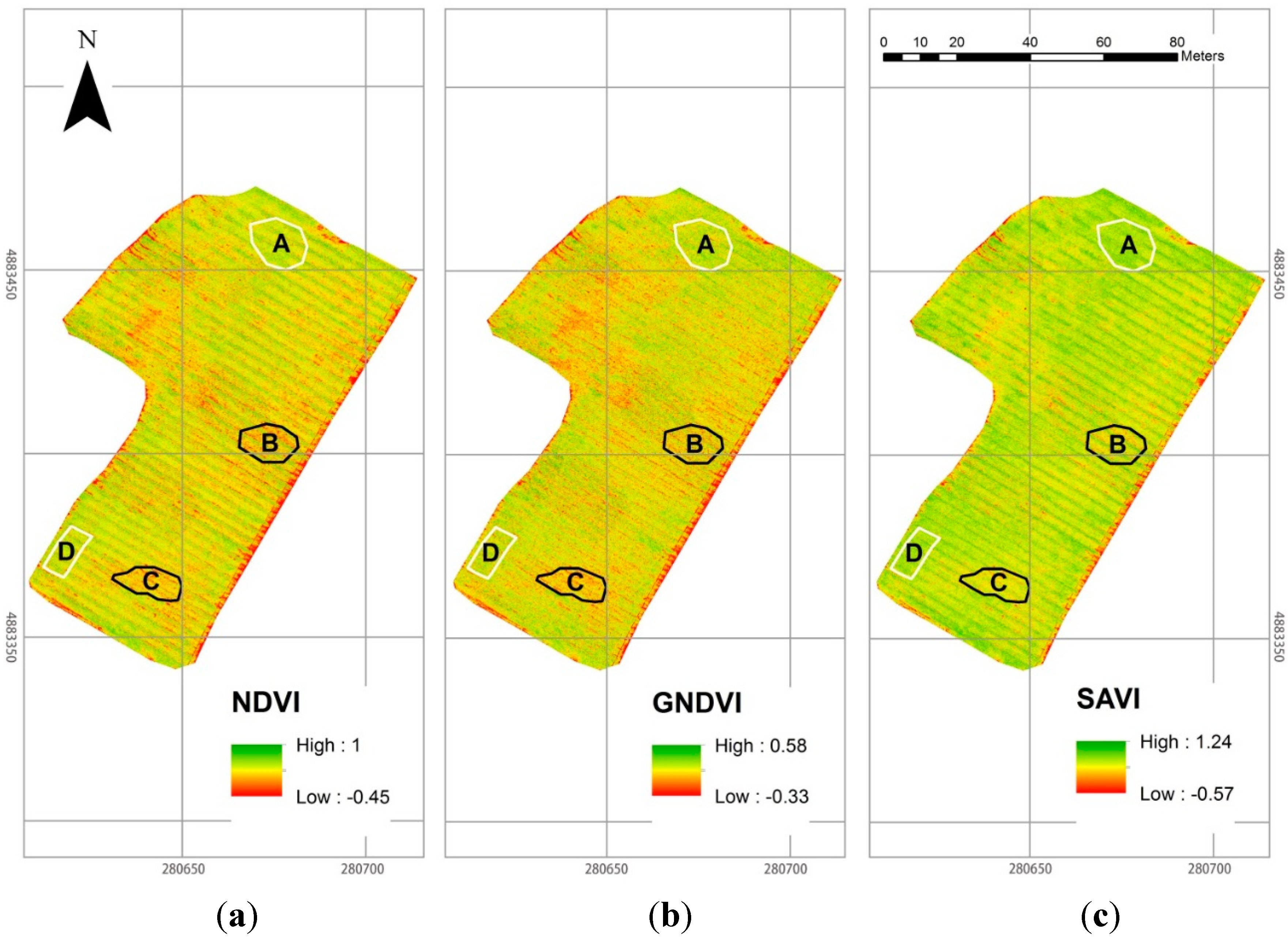
Figure 7. Within the spatial distributions of the NDVI, GNDVI, and SAVI values, the zones with negative behavior are well-recognizable (between orange and red). At the border zones of the vineyard, some red pixels often appear, representing negative values of the index, probably due to the gravel road surrounding the vineyard describing a situation similar to the bare soil. However, for all indices some low values can also be found inside the vineyard. On the other hand, some areas where the vegetation has good vigor attributes for all the indices are also discriminable in the field.
Figure 7. The NDVI (a), GNDVI (b), and SAVI (c, with L = 0.25) maps for the vineyard area. Areas A–D and C–B show zones with high and low VI values, respectively.
Remotesensing 07 04026 g007
Concerning the NDVI index, the found value ranges between −0.45 and 1 (Figure 7a) but only values ranging between 0.4 and 0.9 are compatible with the crop presence. In particular, the vineyard lines are recognized through the higher NDVI values.
Given that the reflectance in green regions is higher than in the red regions, for the GNDVI a different range with respect to the NDVI index was found. The GNDVI map has a maximum at 0.58 whereas the minimum is −0.33 (Figure 7b). From a qualitative analysis, the areas with high NDVI values match to the areas with high GNDVI value.
For the SAVI computation (Figure 7c), the characteristics of the surveyed vineyard area suggested choosing some low L values (L = 0.25 and L = 0.10). In both case, the resulting maps are similar.
As shown in Figure 7b,c, the GNDVI and SAVI values exceed the traditional known ranges, probably due to:
-
the presence of many shadows (dark areas) between the vineyard lines, which badly affected the result of these indices;
-
the use of Digital Numbers instead of the corresponding reflectance values.
However, in all three maps it is possible to recognize the same spectral discrimination of the areas.
To confirm these qualitative considerations, a statistical analysis was performed using all vegetation index maps. Four areas of interest, named A, B, C, and D, were selected inside the vineyard and highlighted with different colors (Figure 7). The white polygons indicate the large index value zones whereas the black polygons cover lower index value.
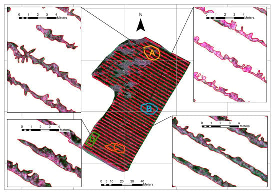
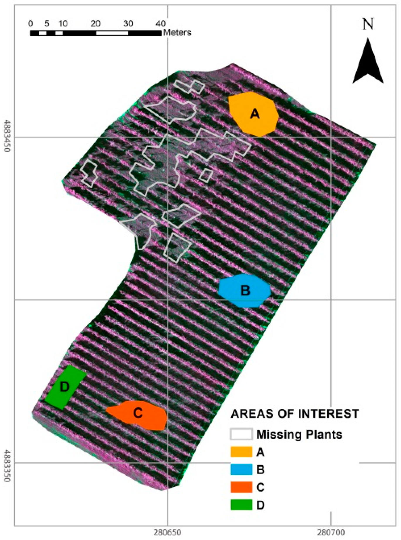
It is important to notice that the vineyard crop has a lack of plants in some areas, especially in the northwest zone (Figure 8). In these areas, low VI values have been derived, again describing a situation similar to the bare soil.
Figure 8. Map of the no-vine plant zones and the areas of interest used for the statistical analysis.
Remotesensing 07 04026 g008
Area A and Area D cover a region with better vegetation conditions, while Area B and Area C include pixels with lower NDVI values. For each area, basic statistics of indices values, i.e., Mean (m) and Standard Deviation (σx), were calculated (Table 5). In particular, the mean NDVI value reflects a mean productivity and biomass, whereas the standard deviation represents a measure of the spatial variability in productivity [24]. The mean value classifications for all indices agree with the previous qualitative discrimination, confirming that the health condition of areas A and D is better than B and C.
Table 5. Mean and Standard Deviation of sample areas A, B, C, and D.
NDVI
AreaN° PixelMeanStandard Deviation
A62,5380.700.09
B49,8960.630.13
C44,8440.610.10
D34,4690.690.10
GNDVI
AreaN° PixelMeanStandard Deviation
A62,5380.260.04
B49,8960.230.06
C44,8440.220.05
D34,4690.260.05
SAVI
AreaN° PixelMeanStandard Deviation
A62,5380.870.12
B49,8960.780.16
C44,8440.760.13
D34,4690.860.13
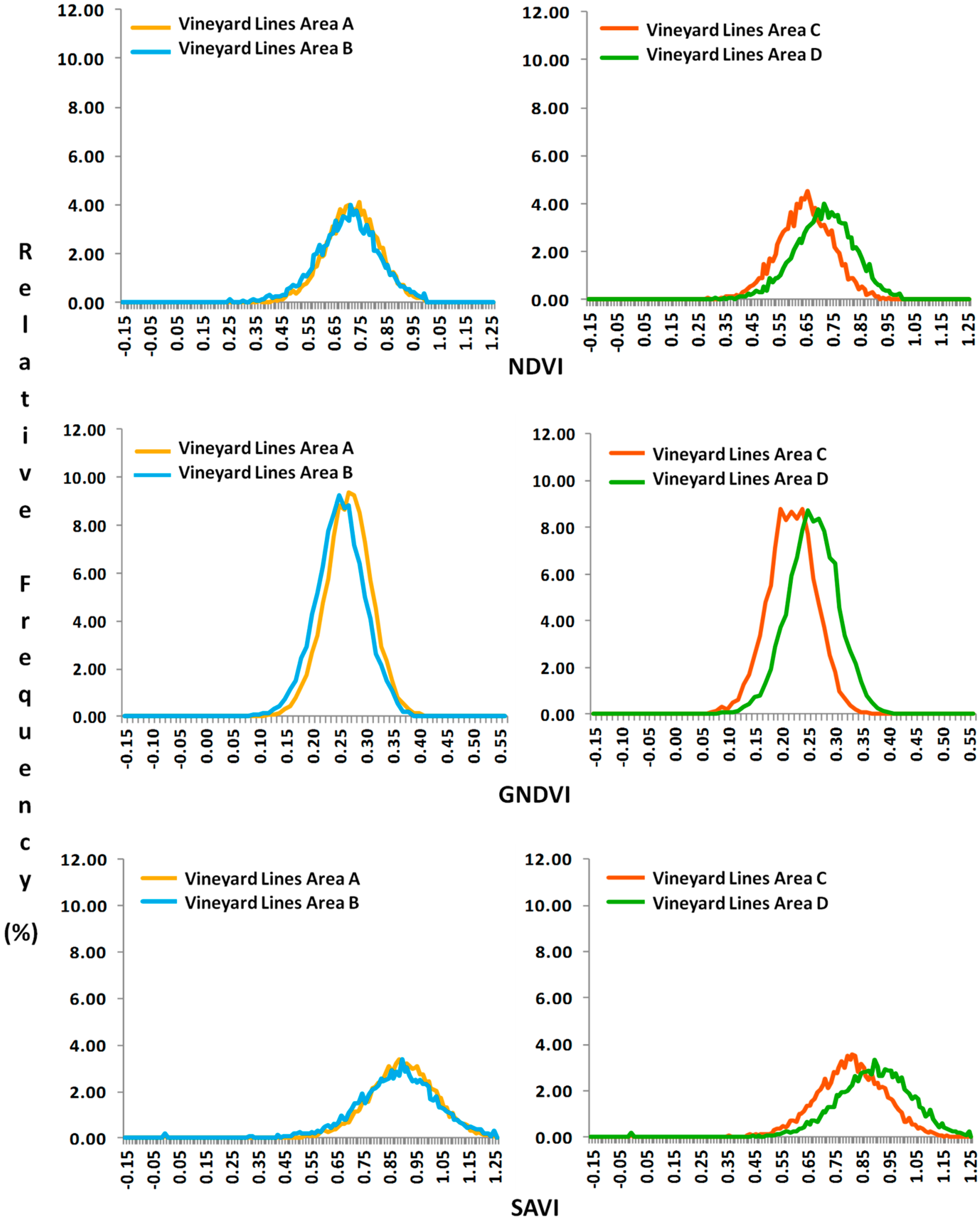
However, as the previous statistic parameters are not able to fully explain the data distributions, in order to satisfy the needs of precision farming techniques, the relative frequency histogram of VI values were plotted for each area (Figure 9). To avoid a histogram overlap and to provide a better understanding, two different graphs were drawn, one relating to areas A and B and the other relating to C and D. For all VI, the graphics show that the pixels belonging to areas A and B are distributed over higher VI values with respect to C and D, confirming again the previous findings.
As mentioned before, the high-resolution contents of the UAV images allow us to detect many details and features normally not visible in low-resolution aerial or satellite imagery. In the analyzed vineyard area, several covers are included besides grapevines, i.e., ground vegetation, wood, shadows, etc. Thus, to eliminate the spectral disturbances of these coverages, sub-areas were selected with a careful manual digitalization of the vineyard lines in order to separate the real cultivated areas from other parts (Figure 10).
For each sub-area, basic statistics of VI values, i.e., Mean (m) and Standard Deviation (σx), were calculated (Table 6). In particular for area B, the mean VI value increase is approximately 13% for the NDVI, about 9% for the GNDVI and about 16% for the SAVI, while for other areas the increase never exceeds 7% (A and C areas always remain below 4%). These results indicate that actually in area B, the plants of the vineyard lines have a healthy state close to that of the plants in the best areas found previously (A and D). This consideration differs from the assessment made in the previous analysis, which referred to the whole areas of interest, demonstrating the advantage of using high-resolution images and selecting only areas with cultivation.
Figure 9. Relative frequency histograms of NDVI, GNDVI, SAVI indices, and values for areas A, B, C, and D. Given the different nature of the GNDVI index, a different range was used for the horizontal axis of the graph.
Remotesensing 07 04026 g009
Finally, the relative frequency histograms of the sub-areas (Figure 11) confirmed that the plants of Area C have a worse vegetative state than that of the vines included in the other areas of interest.
Figure 10. The manually digitized vineyard lines for the areas under investigation (A, B, C, D) to compute the VI only inside the cultivated zones and eliminate possible spectral disturbs from ground vegetation, wood, shadows, etc.
Remotesensing 07 04026 g010
Table 6. Mean and Standard Deviation of sample areas A, B, C, and D.
NDVI
AreaN° PixelMeanStandard Deviation
A11,7500.720.10
B73170.700.12
C93990.650.10
D95840.720.11
GNDVI
AreaN° PixelMeanStandard Deviation
A11,7500.260.04
B73170.250.05
C93990.210.04
D95840.250.05
SAVI
AreaN° PixelMeanStandard Deviation
A11,7500.900.13
B73170.870.16
C93990.810.13
D95840.890.14
Figure 11. Relative frequency histograms of NDVI, GNDVI, SAVI, and values for areas A, B, C, and D. Given the different nature of the GNDVI index, a different range was used for the horizontal axis of the graph.
Remotesensing 07 04026 g011
From this analysis, it is possible to conclude that better health conditions are visible in the vineyard plants contained in areas A and D, while in B the vegetation state is slightly worse. Instead, the C area shows the more worrying situation. The local vineyard farmer confirmed that, being a biological culture, the vineyard is subject to attack by various pests/fungi, including especially Armillaria mellea and the “Grapevine trunk diseases”. In fact, these are the cause of plant removal in the northwest area of the vineyard. The first is a plant pathogen that causes Armillaria root rot in many plant species and produces mushrooms around the base of infected trees. The symptoms appear in the crowns of infected trees as discolored foliage, reduced growth, dieback of the branches, and death [38]. Grapevine trunk diseases are a set of vine diseases caused by fungal species that colonize the lymph vessels and the wood, compromising the translocation of water and nutrients from the roots to the aerial part of the plant. The fungus produces toxins that cause the chlorotic and necrotic stains on the leaves. In grapes it is accompanied by the appearance of purplish spots on the berries [39]. Both diseases are spread over the entire vineyard. However, since the trees that are already under stress are more likely to be attacked, the B area and in particular the C area are more vulnerable to these problems. In fact, these zones have a deficiency of fertilizer. The reason is a depression that has been backfilled in the past, but, despite having a similar composition to the rest of the ground below the vineyard, a lower intake of fertilizer was found.
Finally, the different behavior between area B and C is probably due to the irregular appearance of “Grapevine trunk diseases” symptoms from year to year. Often, the symptomatic plants during a season cannot manifest symptoms for several consecutive years, thus continuing to have the normal production of healthy plants.

5.2. The Tomato Crop

The NDVI, GNDVI, and SAVI indices were computed on the available orthoimage and the extracted VI maps are shown on Figure 12. Compared to the vineyard, in herbaceous crops such as tomatoes the VI analysis is more complex. Indeed, between plants the growth is not uniform and the vegetation distribution on the ground is not homogeneous, with considerable presence of bare soil. As reported by the farm manager, the cause is the “Bacterial spot” presence strongly spread over the whole crop. Bacterial spot is one of the most devastating diseases of tomato fields due to the action of various bacteria that attack foliage, stems, and fruits. Symptoms begin as small, yellow-green lesions on young leaves, which usually appear deformed and twisted, or as dark lesions on older foliage. Lesions develop rapidly and the diseased leaves drop prematurely, resulting in extensive defoliation, while those leaves that remain on the plants may have a scorched appearance. Fruit spots begin as pale-green, water-soaked areas that eventually become raised, brown, and roughened on tomato fruit. Spots may provide entrance points for various fungal and other bacterial invaders that can cause secondary fruit rots [40].
Within the spatial distributions of the NDVI, GNDVI, and SAVI values, the areas with negative behavior are easily recognizable (between orange and red). In the northwest and southeast border zones of the crop, some red pixels—representing negative index values—appear. The cause is probably the gravel road surrounding the field and leading to a situation similar to the bare soil. However, for all indices some low values can be found also inside the tomatoes’ area. Concerning the ranges of the computed VI, the same problem encountered for the vineyard occurs for the tomato crop, too. In particular, the GNDVI and SAVI values exceed the traditional known ranges, probably due to the use of Digital Numbers instead of the corresponding reflectance values.
Figure 12. The NDVI, GNDVI, and SAVI (L = 0.5) maps for the tomato crop. Areas A and B show zones with high and low VI values, respectively.
Remotesensing 07 04026 g012
Two sample areas (A and B) with different vegetation density were then selected. These areas were statistically analyzed, computing Mean (m) and Standard Deviation (σx) (Table 7). The results suggest that the VI response is better for area A than B. In fact, for the former the average VI values are more than 30% Higher.
Table 7. Mean and standard deviation of the sample areas A and B in the tomato crop.
NDVI
AreaN° PixelMeanStandard Deviation
A107,6380.590.18
B107,8190.450.23
GNDVI
AreaN° PixelMeanStandard Deviation
A107,6380.220.08
B107,8190.170.10
SAVI
AreaN° PixelMeanStandard Deviation
A107,6380.870.27
B107,8190.670.35
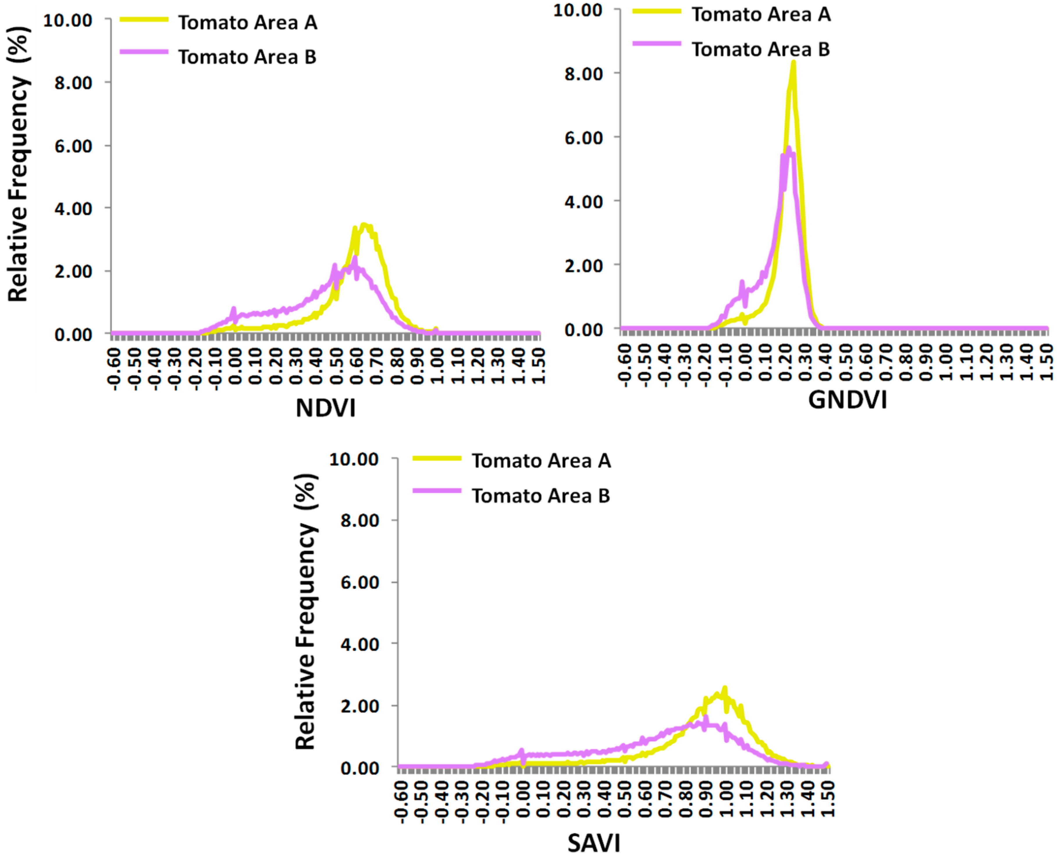
Moreover, considering the relative frequency histograms (Figure 13), it is evident that a greater number of pixels in area B fall on lower values than in area A, indicating a worse health condition. However, it is necessary to emphasize that for tomato cultivation treatments are suspended some time before harvesting; this occurred in this case a few days after the UAV survey. Since, at this stage, some plants continue growth while others will dry on the soil, the decrease of the values of the indexes could not be linked to the state of health only.
Figure 13. Relative frequency histograms of NDVI, GNDVI, and SAVI for areas A and B in the tomato crop.
Remotesensing 07 04026 g013
Due to the uneven plant distribution on the ground, in the tomato crop case study we could not separate the individual plants through a manual digitization procedure.

6. Discussion and Conclusions

This paper reports some analyses of UAV-based precision farming applications, demonstrating the great potential of high-resolution UAV data and photogrammetric techniques applied in the agriculture framework to collect multispectral images (G, R, NIR) and evaluate different Vegetation Indices (VI). VI maps were derived using a multispectral camera flown on two different cultivation types: vineyard and tomatoes. For every dataset, using automated photogrammetric procedures, triband orthoimages were produced and analyzed in relation to some common vegetation indices to demonstrate the flexibility and pertinence of photogrammetric reconstruction in the farming environment. Due to missing ground measurements (no spectral calibration of the data), the VI were computed only based on DN, thus delivering mainly qualitative results—in any case, a good description of the crop conditions.
Nowadays the real need in precision farming is for management strategies that could help farmers in improving crop production and also for a significant saving on products such as fertilizers and pesticides—with a considerable reduction of environmental pollution. In this paper we reported that a UAV approach could reliably deliver VI, showing which are the healthy or unhealthy portions of a cultivated field. With the help of this information, possibly coupled with spectral calibration data, a farmer could locate the plants with worse response to the VI, and take some decision to save the part of the crop production that was in danger. The great flexibility and potentialities of UAVs allow us to obtain fast, multi-temporal, high-resolution, and rigorous representation of VI at low costs. That information, joined with other data coming from multiple sources, e.g., meteorology and agronomy, should simplify the decision-making process in the agricultural sector.
Undoubtedly high-resolution UAV images represent a fast, reliable, and economic resource in crop assessment and could possibly even remove the need for ground inspections entirely. However, the presented experiments highlighted some issues related to the transfer of multispectral remote sensing techniques to the UAV field. In fact, the traditional and well-established procedures able to provide VI from remotely sensed imagery were developed for airborne and satellite datasets with typical GSDs of some meters. Moreover, the unavailability of standard tools that do not require ground measurements to convert the DN values to reflectance values complicates the use of the commonest image processing software and the result interpretation. Therefore, using high-resolution contents from UAV data, more focused analyses were performed only on the cultivated areas, excluding ground, shadows, etc. This has shown how VI maps significantly change. Another constraint is the limited number of spectral bands provided by the used Tetracam ADC Micro camera, which is limiting some vegetation analyses (e.g., humidity content). Better multi- and hyper-spectral sensors could be employed, like the Tetracam Mini-MCA or the Headwall Micro-Hyperspec, for example.
Nevertheless, the UAV approach for precision farming is in constant evolution and represents an extremely dynamic sector. The literature shows that in the future the material and methods related to this approach will be intensively used. The main limitation of our approach was the lack of ground radiometric measures, which could gave a better quantitative representation of the ground situation. On the other hand we reported experiments on two different types of cultivated areas with various VI, showing how useful information can be derived with a fast and low-cost approach.

Acknowledgments

The work was accomplished during Sebastian Candiago’s internship at the 3D Optical Metrology unit (3DOM) of the Bruno Kessler Foundation (FBK) in Trento, Italy. All authors are thankful to the La Quercia farm in Sorrivoli (Cesena, Italy), owned by Maurizio Fiuzzi, for the courtesy of working in the vineyard and to the farm of Francis Ravaioli in San Bartolo (Ravenna, Italy) for the courtesy of operating within the field of tomatoes.

Author Contributions

All authors equally participated in the realization of the research work, in particular: Marco Dubbini and Mario Gattelli conducted the UAV and GNSS surveys as well as the processing of the necessary GCP coordinates; Fabio Remondino performed all the photogrammetric processing on the multispectral data; Sebastian Candiago and Michaela De Giglio analyzed the obtained multispectral results and produced the vegetation indices maps and analyses concerning the precision farming domain. All the authors equally contributed in the paper writing.

Conflicts of Interest

The authors declare no conflict of interest.

References

  1. Santhosh, K.S.; Soizik, L.; Grant, M.C.; George, A.S. Remote sensing applications for precision agriculture: A learning community approach. Remote Sens. Environ. 2003, 88, 157–169. [Google Scholar] [CrossRef]
  2. David, J.M. Twenty five years of remote sensing in precision agriculture: Key advances and remaining knowledge gaps. Biosyst. Eng. 2013, 114, 358–371. [Google Scholar] [CrossRef]
  3. National Research Council. Precision Agriculture in the 21st Century; National Academy Press: Washington, DC, USA, 1997; p. 149.
  4. Nebiker, S.; Annen, A.; Scherrer, M.; Oesch, D. A light-weight multispectral sensor for micro UAV—Opportunities for very high resolution airborne remote sensing. In International Archives of the Photogrammetry, Remote Sensing and Spatial Information Sciences; International Society for Photogrammetry and Remote Sensing (ISPRS): Beijing, China, 2008; Volume 37, (B1). [Google Scholar]
  5. Nex, F.; Remondino, F. UAV for 3D mapping application: A review. Appl. Geomat. 2014, 6, 1–15. [Google Scholar] [CrossRef]
  6. Colomina, I.; Molina, P. Unmanned aerial systems for photogrammetry and remote sensing: A review. ISPRS J. Photogramm. Remote Sens. 2014, 92, 79–97. [Google Scholar] [CrossRef]
  7. Guo, T.; Kujirai, T.; Watanabe, T. Mapping crop status from an unmanned aerial vehicle for precision agriculture applications. In International Archives of the Photogrammetry, Remote Sensing and Spatial Information Sciences; Volume 39, (B1), Melbourne, Australia, 2012. [Google Scholar]
  8. Primicerio, J.; Di Gennaro, S.F.; Fiorillo, E.; Genesio, L.; Lugato, E.; Matese, A.; Vaccari, F.P. A flexible unmanned aerial vehicle for precision agriculture. Precis. Agric. 2012, 13, 517–523. [Google Scholar] [CrossRef]
  9. Turner, D.; Lucieer, A.; Watson, C. Development of an unmanned aerial vehicle (UAV) for hyper resolution vineyard mapping based on visible, multispectral, and thermal imagery. In Proceedings of 34th International Symposium on Remote Sensing of Environment, Sydney, Australia, 10–15 April 2011.
  10. Bendig, J.; Bolten, A.; Bareth, G. Introducing a low-cost mini-UAV for thermal- and multispectral-imaging. Int. Arch. Photogramm. Remote Sens. Spat. Inf. Sci. 2012, 39(B1), 345–349. [Google Scholar]
  11. Grenzdörffer, G.J.; Engel, A.; Teichert, B. The photogrammetric potential of low-cost UAVs in forestry and agriculture. Int. Arch. Photogramm. Remote Sens. Spat. Inf. Sci. 2008, 37(B1), 1207–1214. [Google Scholar]
  12. Ouédraogo, M.M.; Degré, A.; Debouche, C.; Lisein, J. The evaluation of unmanned aerial system-based photogrammetry and terrestrial laser scanning to generate DEMs of agricultural watersheds. Geomorphology 2014, 214, 339–355. [Google Scholar] [CrossRef]
  13. Westoby, M.J.; Brasington, J.; Glasser, N.F.; Hambrey, M.J.; Reynolds, J.M. “Structure-from-motion” photogrammetry: A low-cost, effective tool for geoscience applications. Geomorphology 2012, 179, 300–314. [Google Scholar] [CrossRef] [Green Version]
  14. Mathews, A.J.; Jensen, J.L.R. Visualizing and quantifying vineyard canopy LAI using an unmanned aerial vehicle (UAV) collected high density structure from motion point cloud. Remote Sens. 2013, 5, 2164–2183. [Google Scholar] [CrossRef]
  15. Matese, A.; Capraro, F.; Primicerio, J.; Gualato, G.; Di Gennaro, S.F.; Agati, G. Mapping of vine vigor by UAV and anthocyanin content by a non-destructive fluorescence technique. In Precision Agriculture; Wageningen Academic Publishers: Lleida, Spain, 2013; pp. 201–208. [Google Scholar]
  16. Agüera, F.; Carvajal, F.; Pérez, M. Measuring sunflower nitrogen status from an unmanned aerial vehicle-based system and an on the ground device. In Proceedings of the Conference on Unmanned Aerial Vehicle in Geomatics, Zurich, Switzerland, 14–16 September 2011; Volume 38.
  17. Honkavaara, E.; Kaivosoja, J.; Mäkynen, J.; Pellikka, I.; Pesonen, L.; Saari, H.; Salo, H.; Hakala, T.; Marklelin, L.; Rosnell, T. Hyperspectral reflectance signatures and point clouds for precision agriculture by light weight UAV imaging system. In Proceedings of the XXII ISPRS Congress, Melbourne, Australia, 25 August–1 September 2012; Volume I-7.
  18. Pölönen, I.; Saari, H.; Kaivosoja, J.; Honkavaara, E.; Pesonen, L. Hyperspectral imaging based biomass and nitrogen content estimations from light-weight UAV. Proc. SPIE 2013, 8887. [Google Scholar] [CrossRef]
  19. Zarco-Tejada, P.J.; González-Dugo, V.; Berni, J.A.J. Fluorescence, temperature and narrow-band indices acquired from a UAV platform for water stress detection using a micro-hyperspectral imager and a thermal camera. Remote Sens. Environ. 2012, 117, 322–337. [Google Scholar] [CrossRef]
  20. Zarco-Tejada, P.J.; Catalina, A.; González, M.R.; Martín, P. Relationships between net photosynthesis and steady-state chlorophyll fluorescence retrieved from airborne hyperspectral imagery. Remote Sens. Environ. 2013, 136, 247–258. [Google Scholar] [CrossRef]
  21. Gutierrez-Rodriguez, M.; Escalante-Estrada, J.A.; Rodriguez-Gonzalez, M.T. Canopy reflectance, stomatal conductance, and yield of Phaseolus vulgaris L. and Phaseolus coccinues L. under saline field conditions. Int. J. Agric. Biol. 2005, 7, 491–494. [Google Scholar]
  22. Bachmanna, F.; Herbstb, R.; Gebbersc, R.; Hafnera, V.V. Micro UAV based georeferenced orthophoto generation in VIS+NIR for precision agriculture. In Proceedings of the UAV-g2013, Rostock, Germany, 4–6 September 2013; Volume XL-1/W2.
  23. Kelcey, J.; Lucieer, A. Sensor correction and radiometric calibration of a 6-band multispectral imaging sensor for UAV remote sensing. In Proceedings of the 2012 XXII ISPRS Congress, Melbourne, Australia, 25 August–1 September 2012; Volume 39.
  24. Rouse, J.W.; Haas, R.H.; Schell, J.A.; Deering, D.W. Monitoring vegetation systems in the Great Plains with ERTS. In Proceedings of the Third ERTS Symposium; NASA: Washington, DC, USA; 10–14 December 1973, NASA SP-351; pp. 309–317.
  25. Pettorelli, N.; Vik, J.O.; Mysterud, A.; Gaillard, J.M.; Tucker, C.J.; Stenseth, N.C. Using the satellite-derived NDVI to assess ecological responses to environmental change. Trends Ecol. Evol. 2005, 20, 503–510. [Google Scholar] [CrossRef] [PubMed]
  26. Weier, J.; Herring, D. Measuring Vegetation (NDVI & RVI), 1999. Available online: http://Earthobservatory.nasa.gov (accessed on 17 November 2014).
  27. Gitelson, A.A.; Kaufman, Y.J.; Merzlyak, M.N. Use of a green channel in remote sensing of global vegetation from EOS-MODIS. Remote Sens. Environ. 1996, 58, 289–298. [Google Scholar] [CrossRef]
  28. Hunt, E.R.J.; Hively, W.D.; Daugtry, C.S.T.; McCarty, G.W. Remote sensing of crop leaf area index using unmanned airborne vehicles. In Proceedings of the Pecora 17 Conference, American Society for Photogrammetry and Remote Sensing, Denver, Colorado, 18–20 November 2008.
  29. Huete, A.R. A soil adjusted vegetation index (SAVI). Remote Sens. Environ. 1988, 25, 295–309. [Google Scholar] [CrossRef]
  30. SAL Engineering S.R.l., Modena, Italy. Available online: http://www.salengineering.it/ (accessed on 2 November 2014).
  31. Tetracam Inc., Chatsworth, CA, USA. Available online: http://tetracam.com/ (accessed on 2 November 2014).
  32. Turner, D.; Lucieer, A.; Malenovsky, Z.; King, D.H.; Robinson, S.A. Spatial co-registration of ultra-high resolution visible, multispectral and thermal images acquired with a micro-UAV over Antarctic moss beds. Remote Sensing. 2014, 6, 4003–4024. [Google Scholar] [CrossRef]
  33. Huang, J.; Thomson, S.J.; Lan, J.; Maas, S.J. Multispectral imaging systems for airborne remote sensing to support agricultural production management. Int. J. Agric. Biol. Eng. 2010, 3, 50–62. [Google Scholar]
  34. Venturi, S.; Di Francesco, S.; Materazzi, F.; Manciola, P. UAV and GIS integrated vegetation analysis of Trasimeno Lake. In Proceedings of 15th World Lake Conference, Perugia, Italy, 1–5 September 2014; pp. 220–224.
  35. San Jose Navigation, Inc., Taiwan. Available online: http://www.sanav.com (accessed on 12 November 2014).
  36. Remondino, F.; Fraser, C. Digital camera calibration methods: Considerations and comparisons. Int. Arch. Photogramm. Remote Sens. Spat. Inf. Sci. 2006, 36, 266–272. [Google Scholar]
  37. Remondino, F.; Spera, M.G.; Nocerino, E.; Menna, F.; Nex, F. State of the art in high density image matching. Photogramm. Rec. 2014, 29, 144–166. [Google Scholar] [CrossRef]
  38. Williams, R.E.; Shaw, C.G.; Wargo, P.M.; Sites, W.H. Armillaria Root Disease. Available online: http://www.na.fs.fed.us/spfo/pubs/fidls/armillaria/armillaria.htm (accessed on 10 January 2015).
  39. Niekerk, J.M.; Fourie, P.H.; Halleen, F.; Crous, P.W. Botryosphaeria spp. as grapevine trunk disease pathogens. Phytopathol. Mediterr. 2006, 45, 43–54. [Google Scholar]
  40. Ritchie, D.F. Bacterial spot of pepper and tomato. Available online: http://www.apsnet.org/edcenter/intropp/lessons/prokaryotes/Pages/Bacterialspot.aspx (accessed on 24 November 2014).

