
Forest Fire Smoke Detection Using Back-Propagation Neural Network Based on MODIS Data

Abstract
:
1. Introduction
2. Data Source

| Band | Bandwidth * | Signal to Noise Radio | Spatial Resolution | Primary Use |
|---|---|---|---|---|
| 1 | 620~670 | 128 | 250 m | Land/Cloud/Aerosols Boundaries |
| 2 | 841~876 | 201 | 250 m | Land/Cloud/Aerosols Boundaries |
| 3 | 459~479 | 243 | 500 m | Land/Cloud/Aerosols Properties |
| 4 | 545~565 | 228 | 500 m | Land/Cloud/Aerosols Properties |
| 5 | 1230~1250 | 74 | 500 m | Land/Cloud/Aerosols Properties |
| 6 | 1628~1652 | 275 | 500 m | Land/Cloud/Aerosols Properties |
| 7 | 2105~2155 | 110 | 500 m | Land/Cloud/Aerosols Properties |
| 8 | 405~420 | 880 | 1000 m | Ocean Color/Phytoplankton/Biogeochemistry |
| 9 | 438~448 | 838 | 1000 m | Ocean Color/Phytoplankton/Biogeochemistry |
| 19 | 915~965 | 250 | 1000 m | Atmospheric Water Vapor |
| 20 | 3.66~3.84 | 0.050 | 1000 m | Surface/Cloud Temperature |
| 26 | 1.36~1.39 | 1504 | 1000 m | Cirrus Clouds Water Vapor |
| 31 | 10.78~11.28 | 0.05 | 1000 m | Surface/Cloud Temperature |
| 32 | 11.77~12.27 | 0.05 | 1000 m | Surface/Cloud Temperature |
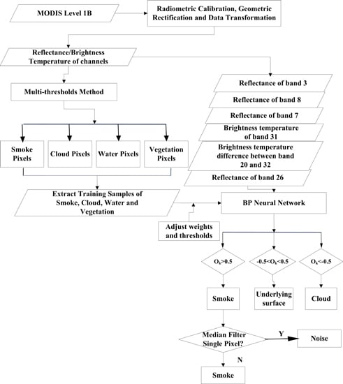
3. Algorithm
- (1)
- Extraction of training samples: Extraction of seasonal training samples of different cover types by multi-threshold method;
- (2)
- Spectral analysis for selecting feature vectors: Spectral analysis of different cover types and selecting feature vectors for input layer of BPNN;
- (3)
- Training of BPNN and Elimination of noise pixels.

3.1. Extraction of Training Samples
3.1.1 Multi-Thresholds for Various Cover Types
3.1.2. Seasonal Training Sample Set

3.2. Spectral Analysis for Selecting Feature Vectors
- (1)
- Spectral analysis of potential smoke plumes and underlying surface;
- (2)
- Spectral analysis of smoke and cloud.
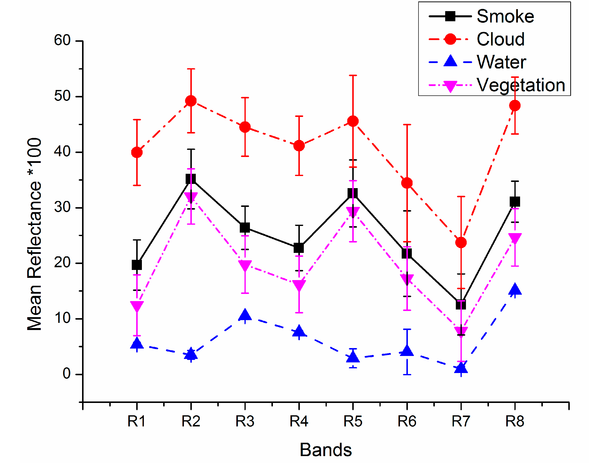
3.2.1. Spectral Analysis of Potential Smoke Plumes and Underlying Surface


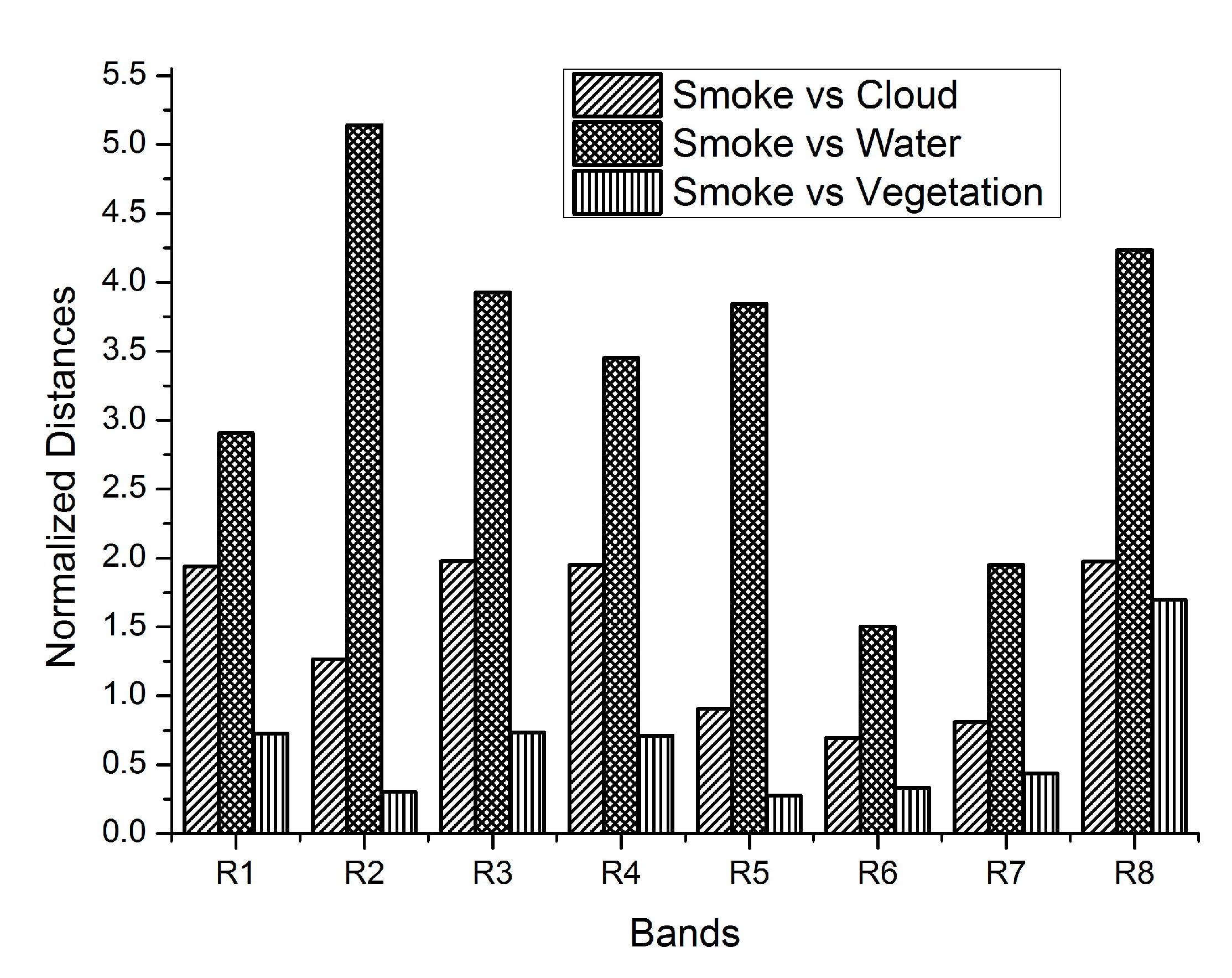
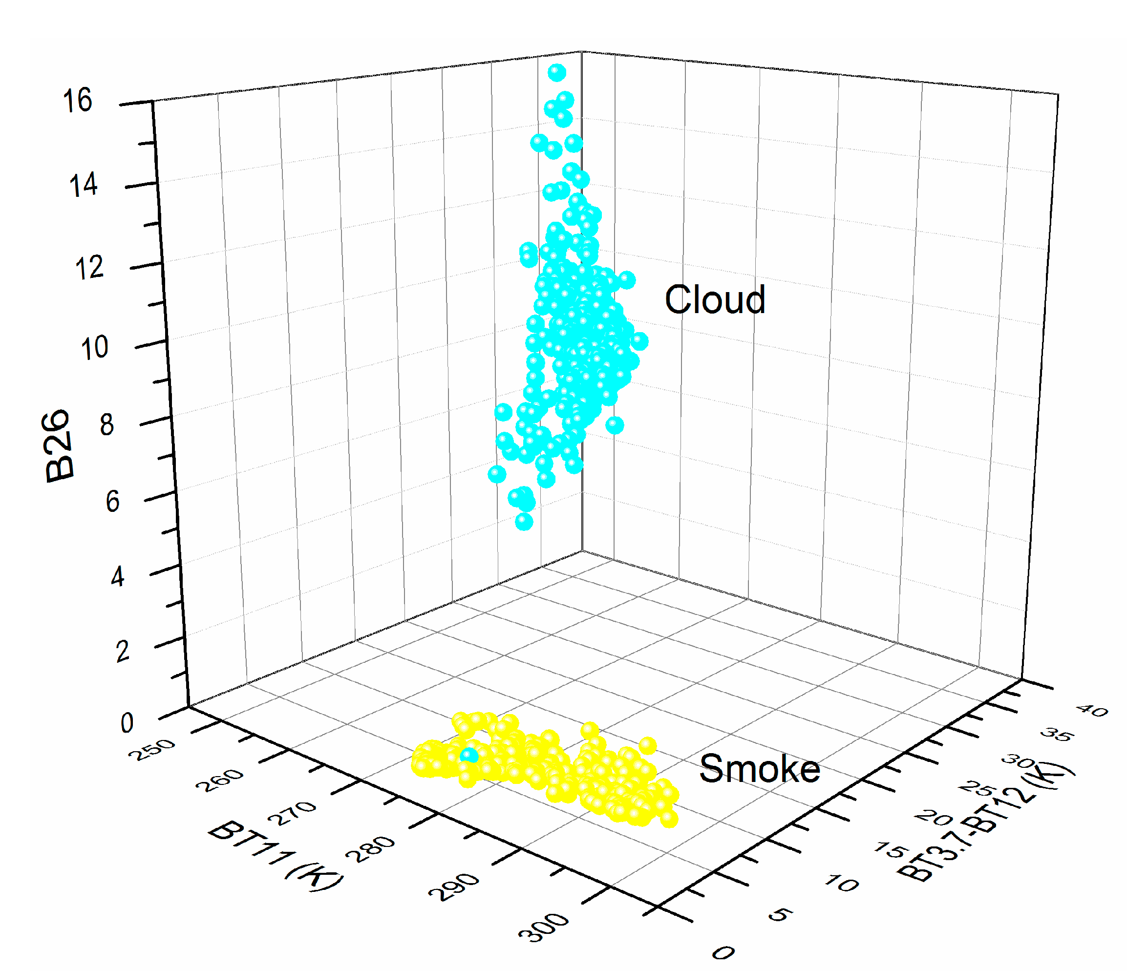
3.2.2. Spectral Analysis of Smoke and Cloud


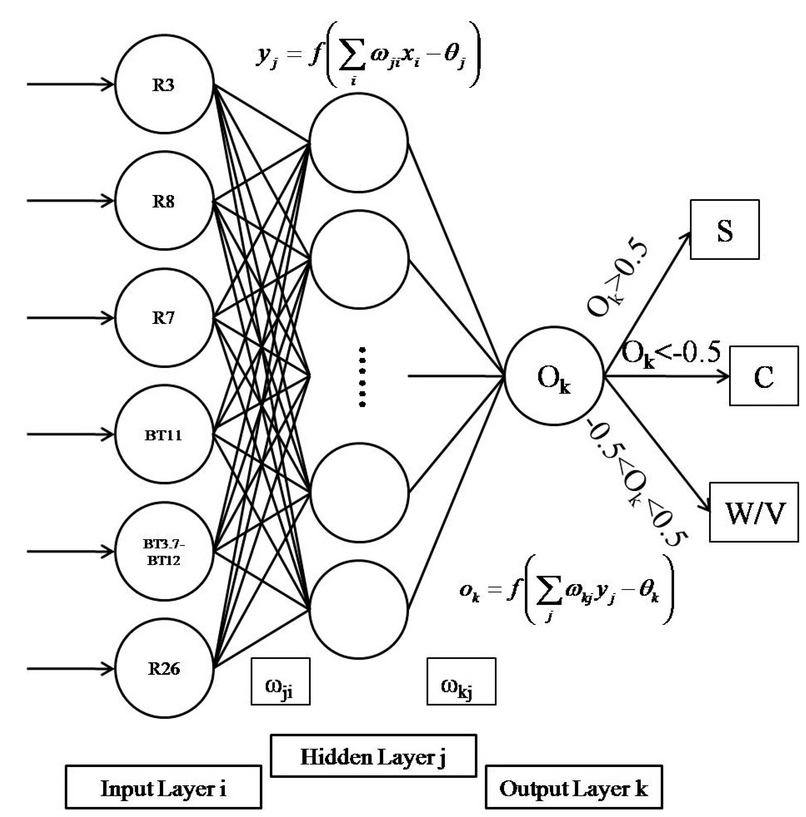
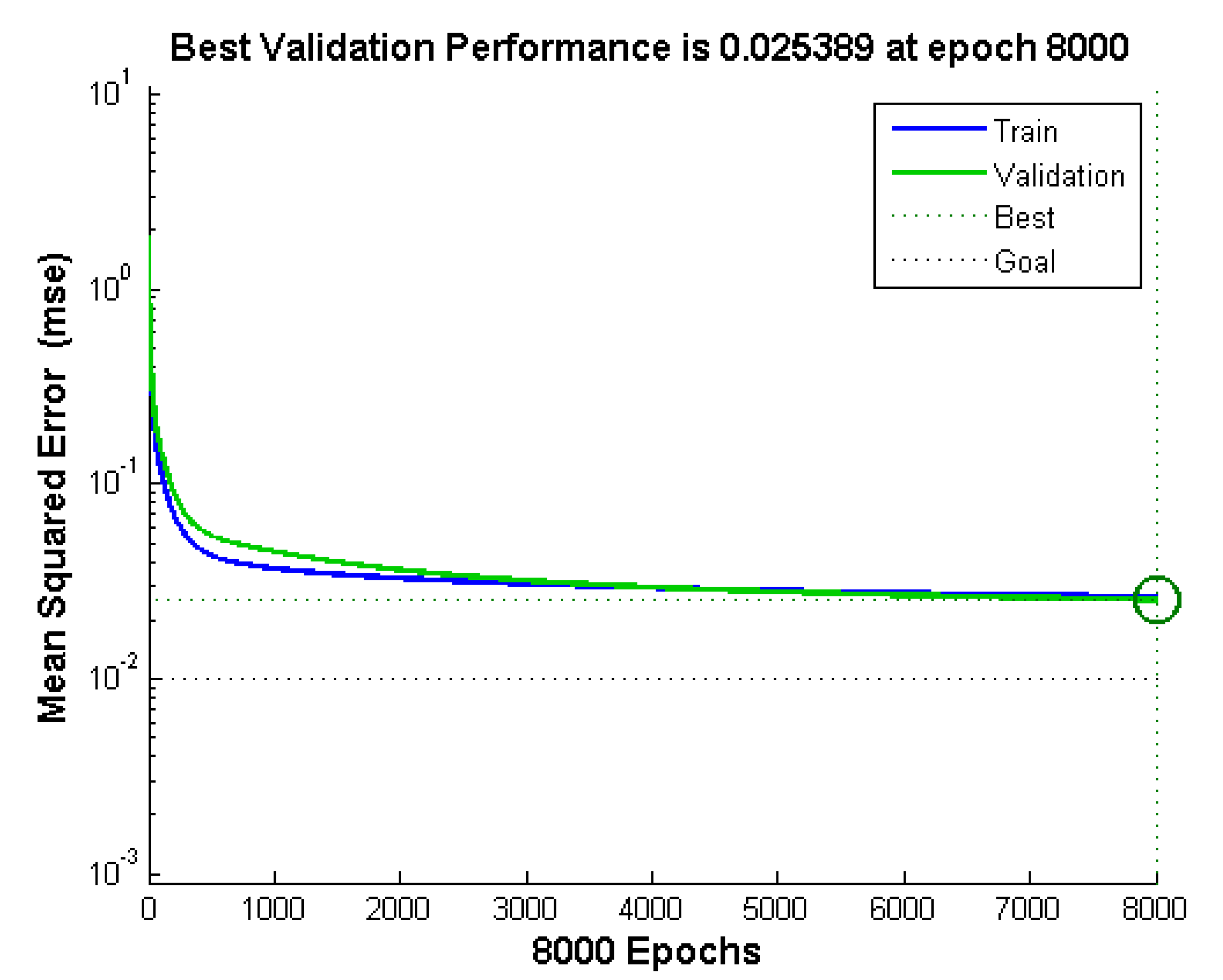
3.3. Training of BPNN and Elimination of Noise Pixels

| Cover Types | Smoke | Underlying Surface | Cloud |
|---|---|---|---|
| Desired Output | 1 | 0 | −1 |

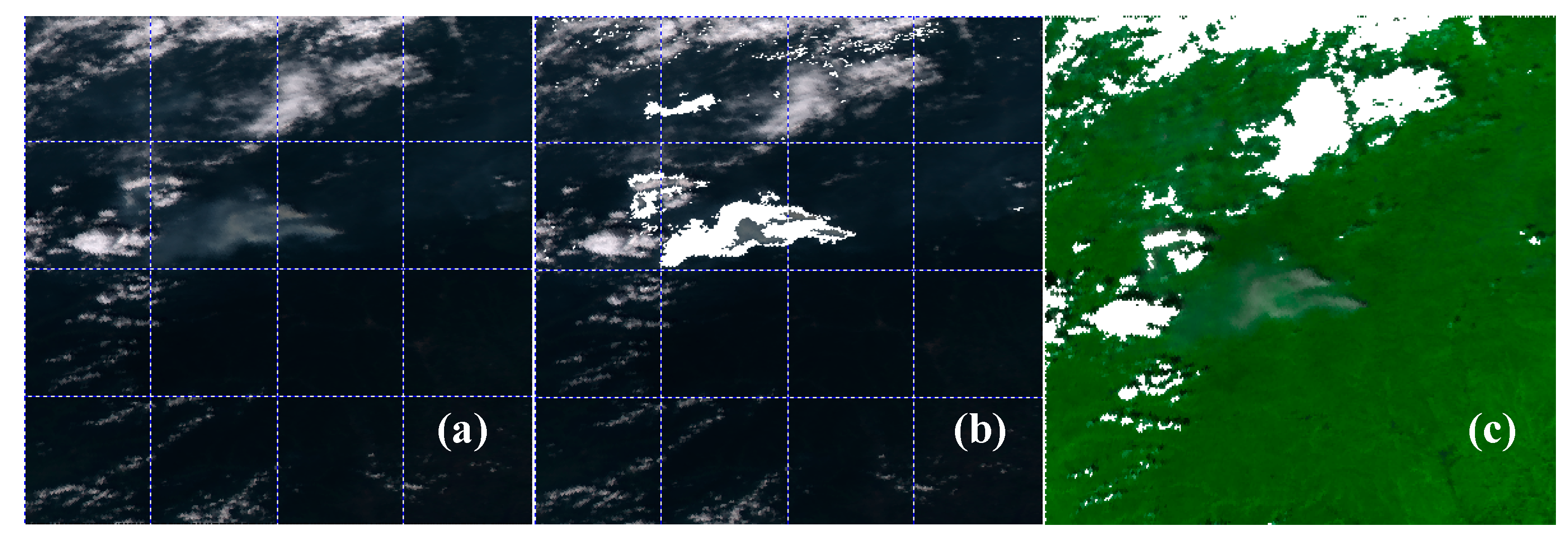
4. Results and Discussion
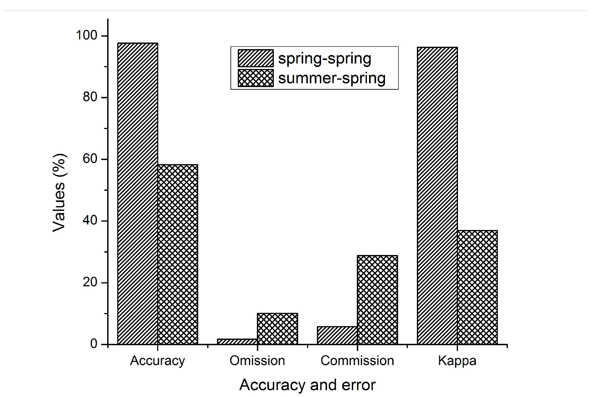
4.1. Accuracy Evaluation of the Algorithm
| Cover Types | Smoke | Underlying Surface | Cloud | Omission Error | Commission Error |
|---|---|---|---|---|---|
| Smoke | 296 | 18 | 0 | 1.66% | 5.73% |
| Underlying Surface | 5 | 521 | 4 | 3.34% | 1.70% |
| Cloud | 0 | 0 | 296 | 1.35% | 0 |
| Overall Accuracy | 97.63% | ||||
| Kappa Coefficient | 96.29% | ||||
| Cover Types | Smoke | Underlying Surface | Cloud | Omission Error | Commission Error |
|---|---|---|---|---|---|
| Smoke | 1178 | 228 | 248 | 10.08% | 28.78% |
| Underlying Surface | 132 | 1151 | 1062 | ||
| Cloud | 0 | 1 | 0 | ||
| Overall Accuracy | 58.23% | ||||
| Kappa Coefficient | 36.92% | ||||

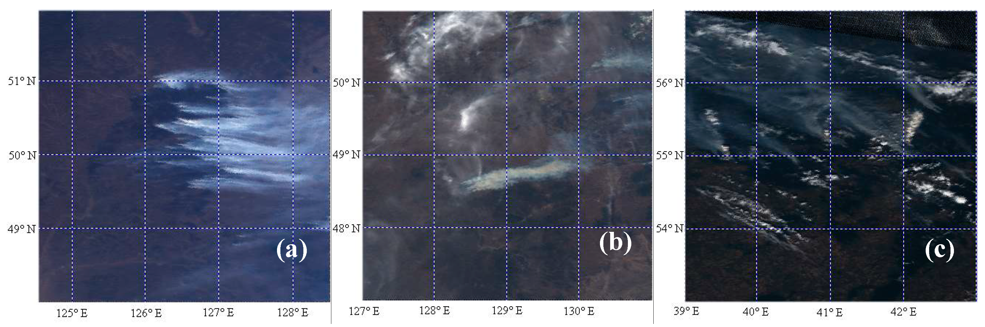
4.2. Seasonal Applicability of the Algorithm

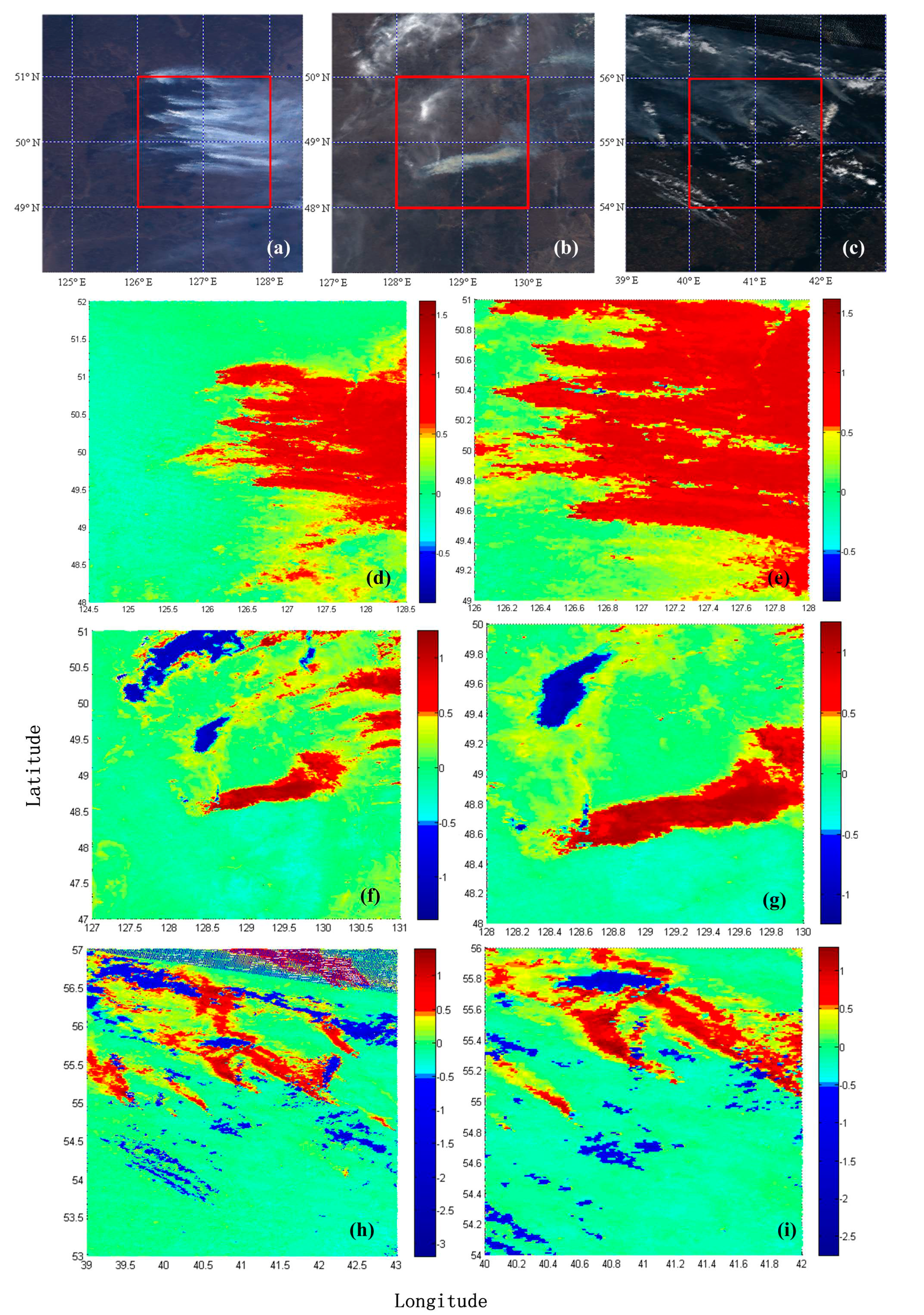
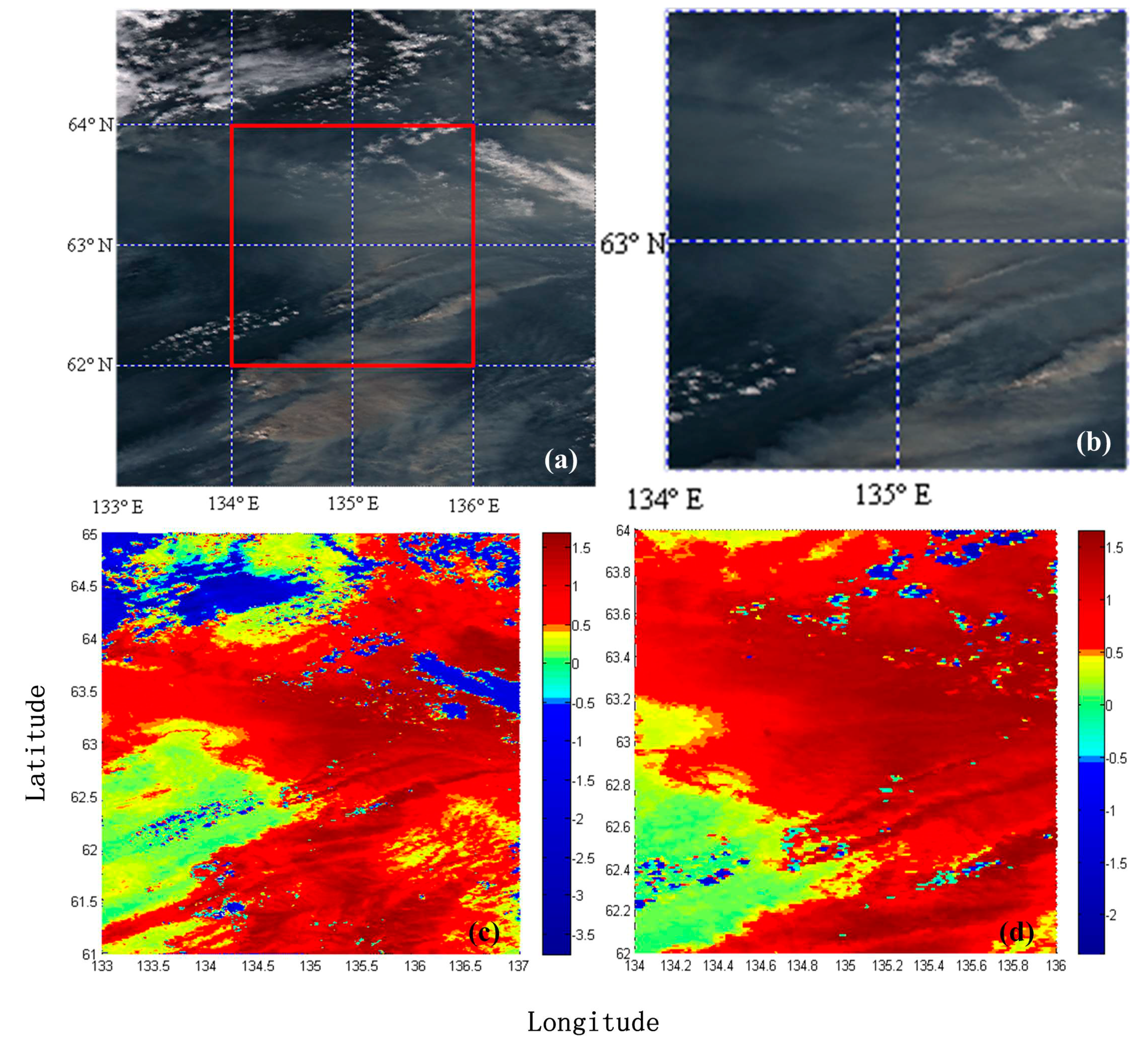
4.3. Robustness of the Algorithm


4.4. Results of the Multi-Threshold Method

5. Conclusions
Acknowledgements
Author Contributions
Conflicts of Interest
References
- Telesca, L.; Kanevski, M.; Tonini, M.; Pezzatti, G.B.; Conedera, M. Temporal patterns of fire sequences observed in canton of Ticino (Southern Switzerland). Nat. Hazard. Earth Syst. 2010, 10, 723–728. [Google Scholar] [CrossRef]
- Kaufman, Y.J.; Fraser, R.S. The effect of smoke particles on clouds and climate forcing. Science 1997, 277, 1636–1639. [Google Scholar] [CrossRef]
- Randerson, J.T.; Liu, H.; Flanner, M.G.; Chambers, S.D.; Jin, Y.; Hess, P.G.; Pfister, G.; Mack, M.C.; Treseder, K.K.; Welp, L.R.; et al. The impact of boreal forest fire on climate warming. Science 2006, 314, 1130–1132. [Google Scholar] [CrossRef] [PubMed]
- Wang, J.; Christopher, S.A.; Nair, U.S.; Reid, J.S.; Prins, E.M.; Szykman, J.; Hand, J.L. Mesoscale modeling of central American smoke transport to the united states: 1. “Top-down” assessment of emission strength and diurnal variation impacts. J. Geophys. Res.: Atmos. 2006, 111. [Google Scholar] [CrossRef]
- Ge, C.; Wang, J.; Reid, J.S. Mesoscale modeling of smoke transport over the Southeast Asian maritime continent: Coupling of smoke direct radiative effect below and above the low-level clouds. Atmos. Chem. Phys. 2014, 14, 159–174. [Google Scholar] [CrossRef]
- Mott, J.A.; Meyer, P.; Mannino, D.; Redd, S.C.; Smith, E.M.; Gotway-Crawford, C.; Chase, E. Wildland forest fire smoke: Health effects and intervention evaluation, Hoopa, California, 1999. Western J. Med. 2002, 176, 157–162. [Google Scholar] [CrossRef]
- Penner, J.E.; Dickinson, R.E.; Oneill, C.A. Effects of aerosol from biomass burning on the global radiation budget. Science 1992, 256, 1432–1434. [Google Scholar] [CrossRef] [PubMed]
- Crutzen, P.J.; Andreae, M.O. Biomass burning in the tropics—Impact on atmospheric chemistry and biogeochemical cycles. Science 1990, 250, 1669–1678. [Google Scholar] [CrossRef] [PubMed]
- Kaskaoutis, D.G.; Kharol, S.K.; Sifakis, N.; Nastos, P.T.; Sharma, A.R.; Badarinath, K.V.S.; Kambezidis, H.D. Satellite monitoring of the biomass-burning aerosols during the wildfires of august 2007 in Greece: Climate implications. Atmos. Environ. 2011, 45, 716–726. [Google Scholar] [CrossRef]
- Duclos, P.; Sanderson, L.M.; Lipsett, M. The 1987 forest fire disaster in California—Assessment of emergency room visits. Arch. Environ. Health 1990, 45, 53–58. [Google Scholar] [CrossRef] [PubMed]
- Shusterman, D.; Kaplan, J.Z.; Canabarro, C. Immediate health-effects of an urban wildfire. Western J. Med. 1993, 158, 133–138. [Google Scholar]
- Li, Z.Q. Influence of absorbing aerosols on the inference of solar surface radiation budget and cloud absorption. J. Climate 1998, 11, 5–17. [Google Scholar] [CrossRef]
- Cahoon, D.R.; Stocks, B.J.; Levine, J.S.; Cofer, W.R.; Pierson, J.M. Satellite analysis of the severe 1987 forest-fires in northern china and southeastern Siberia. J. Geophys. Res.: Atmos. 1994, 99, 18627–18638. [Google Scholar] [CrossRef]
- Prins, E.M.; Feltz, J.M.; Menzel, W.P.; Ward, D.E. An overview of goes-8 diurnal fire and smoke results for scar-b and 1995 fire season in South America. J. Geophys. Res.: Atmos. 1998, 103, 31821–31835. [Google Scholar] [CrossRef]
- Fromm, M.; Alfred, J.; Hoppel, K.; Hornstein, J.; Bevilacqua, R.; Shettle, E.; Servranckx, R.; Li, Z.Q.; Stocks, B. Observations of boreal forest fire smoke in the stratosphere by Poam III, Sage II, and Lidar in 1998. Geophys. Res. Lett. 2000, 27, 1407–1410. [Google Scholar] [CrossRef]
- Chrysoulakis, N.; Herlin, I.; Prastacos, P.; Yahia, H.; Grazzini, J.; Cartalis, C. An improved algorithm for the detection of plumes caused by natural or technological hazards using AVHRR imagery. Remote Sens Environ. 2007, 108, 393–406. [Google Scholar] [CrossRef]
- San-Miguel-Ayanz, J.; Ravail, N.; Kelha, V.; Ollero, A. Active fire detection for fire emergency management: Potential and limitations for the operational use of remote sensing. Nat. Hazards 2005, 35, 361–376. [Google Scholar] [CrossRef]
- Wang, W.T.; Qu, J.J.; Hao, X.J.; Liu, Y.Q.; Sommers, W.T. An improved algorithm for small and cool fire detection using modis data: A preliminary study in the southeastern United States. Remote Sens. Environ. 2007, 108, 163–170. [Google Scholar] [CrossRef]
- Wang, W.T.; Qu, J.J.; Hao, X.J.; Liu, Y.Q. Analysis of the moderate resolution imaging spectroradiometer contextual algorithm for small fire detection. J. Appl. Remote Sens. 2009, 3. [Google Scholar] [CrossRef]
- Liu, C.C.; Kuo, Y.C.; Chen, C.W. Emergency responses to natural disasters using formosat-2 high-spatiotemporal-resolution imagery: Forest fires. Nat. Hazards 2013, 66, 1037–1057. [Google Scholar] [CrossRef]
- Li, Z.Q.; Khananian, A.; Fraser, R.H.; Cihlar, J. Automatic detection of fire smoke using artificial neural networks and threshold approaches applied to AVHRR imagery. IEEE. Trans. Geosci. Remote Sens. 2001, 39, 1859–1870. [Google Scholar] [CrossRef]
- Chung, Y.S.; Le, H.V. Detection of forest-fire smoke plumes by satellite imagery. Atmos. Environ. 1984, 18, 2143–2151. [Google Scholar] [CrossRef]
- Christopher, S.A.; Chou, J. The potential for collocated aglp and erbe data for fire, smoke, and radiation budget studies. Int. J. Remote Sens. 1997, 18, 2657–2676. [Google Scholar] [CrossRef]
- Chrysoulakis, N.; Opie, C. Using NOAA and FY imagery to track plumes caused by the 2003 bombing of Baghdad. Int. J. Remote Sens. 2004, 25, 5247–5254. [Google Scholar] [CrossRef]
- Kaufman, Y.J.; Tucker, C.J.; Fung, I. Remote-sensing of biomass burning in the tropics. J. Geophys. Res.: Atmos. 1990, 95, 9927–9939. [Google Scholar] [CrossRef]
- Randriambelo, T.; Baldy, S.; Bessafi, M. An improved detection and characterization of active fires and smoke plumes in south-eastern Africa and Madagascar. Int. J. Remote Sens. 1998, 19, 2623–2638. [Google Scholar] [CrossRef]
- Baum, B.A.; Trepte, Q. A grouped threshold approach for scene identification in AVHRR imagery. J. Atmos. Ocean. Tech. 1999, 16, 793–800. [Google Scholar] [CrossRef]
- Xie, Y.; Qu, J.J.; Xiong, X.; Hao, X.; Che, N.; Sommers, W. Smoke plume detection in the eastern united states using MODIS. Int. J. Remote Sens. 2007, 28, 2367–2374. [Google Scholar] [CrossRef]
- Zhao, T.X.P.; Ackerman, S.; Guo, W. Dust and smoke detection for multi-channel imagers. Remote Sens. 2010, 2, 2347–2368. [Google Scholar] [CrossRef]
- Xie, Y. Detection of Smoke and Dust Aerosols Using Multi-Sensor Satellite Remote Sensing Measurements; George Mason University: Fairfax, VA, USA, 2009. [Google Scholar]
- Gong, P.; Pu, R.L.; Li, Z.Q.; Scarborough, J.; Clinton, N.; Levien, L.M. An integrated approach to wildland fire mapping of California, USA using NOAA/AVHRR data. Photogramm. Eng. Remote Sens. 2006, 72, 139–150. [Google Scholar] [CrossRef]
- Kaufman, Y.J.; Herring, D.D.; Ranson, K.J.; Collatz, G.J. Earth observing system AM1 mission to earth. IEEE Trans. Geosci. Remote Sens. 1998, 36, 1045–1055. [Google Scholar] [CrossRef]
- Remer, L.A.; Kaufman, Y.J.; Tanre, D.; Mattoo, S.; Chu, D.A.; Martins, J.V.; Li, R.R.; Ichoku, C.; Levy, R.C.; Kleidman, R.G.; et al. The MODIS aerosol algorithm, products, and validation. J. Atmos. Sci. 2005, 62, 947–973. [Google Scholar] [CrossRef]
- Gao, B.-C.; Goetz, A.F.H.; Wiscombe, W.J. Cirrus cloud detection from airborne imaging Spectrometer data using the 1.38 µm water vapor band. Geophys. Res. Lett. 1993, 20, 301–304. [Google Scholar] [CrossRef]
- Gao, B.-C.; Yang, P.; Han, W.; Li, R.-R.; Wiscombe, W.J. An algorithm using visible and 1.38-μm channels to retrieve cirrus cloud reflectances from aircraft and satellite data. IEEE Trans. Geosci. Remote Sens. 2002, 40, 1659–1668. [Google Scholar] [CrossRef]
- NASA: MODIS Level 1 Data, Geolocation, Cloud Mask, and Atmosphere Products. Available online: http://ladsweb.nascom.nasa.gov/ (accessed on 14 December 2014).
- Clark, C.; Canas, A. Spectral identification by artificial neural-network and genetic algorithm. Int. J. Remote Sens 1995, 16, 2255–2275. [Google Scholar] [CrossRef]
- Stroppiana, D.; Pinnock, S.; Gregoire, J.M. The global fire product: Daily fire occurrence from April 1992 to December 1993 derived from NOAA AVHRR data. Int. J. Remote Sens. 2000, 21, 1279–1288. [Google Scholar] [CrossRef]
- Giglio, L.; Descloitres, J.; Justice, C.O.; Kaufman, Y.J. An enhanced contextual fire detection algorithm for MODIS. Remote Sens. Environ. 2003, 87, 273–282. [Google Scholar] [CrossRef]
- Huang, S.F.; Li, J.G.; Xu, M. Water surface variations monitoring and flood hazard analysis in Dongting Lake area using long-term TERRA/MODIS data time series. Nat. Hazards 2012, 62, 93–100. [Google Scholar] [CrossRef]
- Ben-Ze’Ev, E.; Karnieli, A.; Agam, N.; Kaufman, Y.; Holben, B. Assessing vegetation condition in the presence of biomass burning smoke by applying the aerosol-free vegetation index (AFRI) on MODIS images. Int. J. Remote Sens. 2006, 27, 3203–3221. [Google Scholar] [CrossRef]
- Escuin, S.; Navarro, R.; Fernandez, P. Fire severity assessment by using NBR (normalized burn ratio) and NDVI (normalized difference vegetation index) derived from Landsat TM/ETM images. Int. J. Remote Sens. 2008, 29, 1053–1073. [Google Scholar] [CrossRef]
- Telesca, L.; Lasaponara, R. Investigating fire-induced behavioural trends in vegetation covers. Commun. Nonlinear Sci. 2008, 13, 2018–2023. [Google Scholar] [CrossRef]
- Leon, J.R.R.; van Leeuwen, W.J.D.; Casady, G.M. Using MODIS-NDVI for the modeling of post-wildfire vegetation response as a function of environmental conditions and pre-fire restoration treatments. Remote Sens. 2012, 4, 598–621. [Google Scholar] [CrossRef]
- Clerici, N.; Weissteiner, C.J.; Gerard, F. Exploring the use of MODIS NDVI-based phenology indicators for classifying forest general habitat categories. Remote Sens. 2012, 4, 1781–1803. [Google Scholar] [CrossRef] [Green Version]
- Chowdhury, E.H.; Hassan, Q.K. Use of remote sensing-derived variables in developing a forest fire danger forecasting system. Nat. Hazards 2013, 67, 321–334. [Google Scholar] [CrossRef]
- Li, X.L.; Wang, J.; Song, W.G.; Ma, J.; Telesca, L.; Zhang, Y.M. Automatic smoke detection in modis satellite data based on k-means clustering and fisher linear discrimination. Photogramm. Eng. Remote Sens. 2014, 80, 971–982. [Google Scholar]
- Gao, B.C.; Xiong, X.X.; Li, R.R.; Wang, D.Y. Evaluation of the moderate resolution imaging spectrometer special 3.95-mu m fire channel and implications on fire channel selections for future satellite instruments. J. Appl. Remote Sens. 2007, 1. [Google Scholar] [CrossRef]
- Bendor, E. A precaution regarding cirrus cloud detection from airborne imaging spectrometer data using the 1.38-µm water-vapor band. Remote Sens. Environ. 1994, 50, 346–350. [Google Scholar] [CrossRef]
- Hsieh, W.W.; Tang, B.Y. Applying neural network models to prediction and data analysis in meteorology and oceanography. Bull. Am. Meteorol. Soc. 1998, 79, 1855–1870. [Google Scholar] [CrossRef]
- Li, L.M.; Song, W.G.; Ma, J.; Satoh, K. Artificial neural network approach for modeling the impact of population density and weather parameters on forest fire risk. Int. J. Wildland. Fire 2009, 18, 640–647. [Google Scholar] [CrossRef]
- Vasilakos, C.; Kalabokidis, K.; Hatzopoulos, J.; Matsinos, I. Identifying wildland fire ignition factors through sensitivity analysis of a neural network. Nat. Hazards 2009, 50, 125–143. [Google Scholar] [CrossRef]
- Albayrak, A.; Wei, J.; Petrenko, M.; Lynnes, C.; Levy, R.C. Global bias adjustment for MODIS aerosol optical thickness using neural network. J. Appl. Remote Sens. 2013, 7. [Google Scholar] [CrossRef]
- Rumelhart, D.E.; Mcclelland, J.L. Parallel Distributed Processing: Explorations in the Microstructure of Cognition; The MIT Press: Cambridge, MA, USA, 1986. [Google Scholar]
- Bishop, C.M. Neural Networks for Pattern Recognition; Oxford University Press: Oxford, UK, 1995. [Google Scholar]
- Levenberg, K. A method for the solution of certain non-linear problems in least squares. Q. J. Appl. Math. 1944, II, 164–168. [Google Scholar]
- Marquardt, D.W. An algorithm for least-squares estimation of nonlinear parameters. J. Soc. Ind. Appl. Math. 1963, 11, 431–441. [Google Scholar] [CrossRef]
- Taylor, M.; Kazadzis, S.; Tsekeri, A.; Gkikas, A.; Amiridis, V. Satellite retrieval of aerosol microphysical and optical parameters using neural networks: A new methodology applied to the Sahara Desert dust peak. Atmos. Meas. Tech. 2014, 7, 3151–3175. [Google Scholar] [CrossRef] [Green Version]
© 2015 by the authors; licensee MDPI, Basel, Switzerland. This article is an open access article distributed under the terms and conditions of the Creative Commons Attribution license (http://creativecommons.org/licenses/by/4.0/).
Share and Cite
Li, X.; Song, W.; Lian, L.; Wei, X. Forest Fire Smoke Detection Using Back-Propagation Neural Network Based on MODIS Data. Remote Sens. 2015, 7, 4473-4498. https://0-doi-org.brum.beds.ac.uk/10.3390/rs70404473
Li X, Song W, Lian L, Wei X. Forest Fire Smoke Detection Using Back-Propagation Neural Network Based on MODIS Data. Remote Sensing. 2015; 7(4):4473-4498. https://0-doi-org.brum.beds.ac.uk/10.3390/rs70404473
Chicago/Turabian StyleLi, Xiaolian, Weiguo Song, Liping Lian, and Xiaoge Wei. 2015. "Forest Fire Smoke Detection Using Back-Propagation Neural Network Based on MODIS Data" Remote Sensing 7, no. 4: 4473-4498. https://0-doi-org.brum.beds.ac.uk/10.3390/rs70404473