Detecting and Characterizing Active Thrust Fault and Deep-Seated Landslides in Dense Forest Areas of Southern Taiwan Using Airborne LiDAR DEM

Abstract

Steep topographic reliefs and heavy vegetation severely limit visibility when examining geological structures and surface deformations in the field or when detecting these features with traditional approaches, such as aerial photography and satellite imagery. However, a light detection and ranging (LiDAR)-derived digital elevation model (DEM), which is directly related to the bare ground surface, is successfully employed to map topographic signatures with an appropriate scale and accuracy and facilitates measurements of fine topographic features. This study demonstrates the efficient use of 1-m-resolution LiDAR for tectonic geomorphology in forested areas and to identify a fault, a deep-seated landslide, and the regional cleavage attitude in southern Taiwan. Integrated approaches that use grayscale slope images, openness with a tint color slope visualization, the three-dimensional (3D) perspective of a red relief image map, and a field investigation are employed to identify the aforementioned features. In this study, the previously inferred Meilongshan Fault is confirmed as a NE–SW-trending, eastern dipping thrust with at least a 750 m-wide deformation zone. The site where future paleoseismological studies should be performed has been identified, and someone needs to work further on this site. Signatures of deep-seated landslides, such as double ridges, trenches, main escarpments, and extension cracks, are successfully differentiated in LiDAR DEM images through the use of different visualization techniques. Systematic parallel and continuous lineaments in the images are interpreted as the regional cleavage attitude of cleavage, and a field investigation confirms this interpretation.

1. Introduction

Active faults and deep-seated landslides frequently occur in the mountainous regions of Taiwan, which is located in a tectonically active environment and in a sub-tropic climatic zone. When studying active faults and deep-seated landslides, tectonic-geomorphic mapping is an important method because it provides valuable information for analyzing landscape evolution that is caused by tectonic activity and surface geological processes. It is also a major tool for seismic hazard assessment and earthquake geological studies. Valuable data can be obtained from the geomorphology of active faulting and can be used to gather fault-specific information that would allow for determination of its recurrence interval [1,2]. However, heavy vegetation covers present a major problem for tectonic-geomorphic mapping because the dense vegetation obscures the visibility of the underlying landforms.

Many methods are available for detecting surface processes and the reactivations of faults with remote sensing data [3,4,5,6]. Compared with traditional approaches, light detection and ranging (LiDAR) is a relatively new remote sensing technique [7] that uses active laser transmitters and receivers to quickly and accurately acquire elevation data [8]. LiDAR data are used to produce a digital elevation model (DEM), which is directly related to the bare ground surface and provides useful information on fine topographic features that cannot be detected under heavy vegetation and underbrush conditions [9,10,11]. The technique allows a laser signal to penetrate the forest canopy and produce at least a meter-resolution image of how the ground surface would appear if the forest were stripped away. Because of its high resolution and precision, airborne LiDAR has led to a marked growth in terrain information and has facilitated the detection of fine-scale tectonic-geomorphic features required for understanding geological surface processes and the quantitative exploration of the characteristics of tectonic geomorphology [12,13,14,15,16,17]. This technique has recently been used to map fault zones and deep-seated landslides with extraordinary detail and aerial coverage [18,19,20]. Because LiDAR-derived DEMs offer a markedly higher spatial resolution than present topographic maps and aerial photos, they allow us to map the locations of fault traces and deep-seated landslides more accurately than was previously possible.

Zachariasen and his research team [21] used LiDAR-derived DEMs to compile an updated map of active traces along a 38-km stretch of the northern San Andreas Fault in Mendocino and Sonoma Counties. These researchers concluded that LiDAR data have been crucial in identifying lineaments that may be fault traces or fault-related features. Topographic detail well beyond what is possible with aerial imagery is available, and scarps, swales, linear valleys and other fault-related features with a distinct topographic signature are evident in the imagery. Chan et al. [22] applied high-resolution airborne LiDAR data to study a segment of the Hsincheng Fault in northern Taiwan. Their results indicated that it was possible to detect landforms and subtle but important geomorphic features with high precision and clarity. However, other studies reported that certain small tectonic breaks could not be identified with the 1- to 2-m-resolution DEM in areas with heavy vegetation and complicated topography [23]. The presence of dense vegetation and topographic complexities reduced the number of ground laser strikes, thereby generating low-density ground data that failed to capture subtle geomorphic features. Chigira et al. [24] analyzed LiDAR-derived high-resolution DEMs captured before and after Typhoon Talas in 2011 and found that 10 large catastrophic landslides were preceded by gravitational slope deformation. In the LiDAR-derived DEMs that was generated before the typhoon, small scarps can be detected near their future crowns prior to the slide. Their study noted that LiDAR-derived DEMs provide invaluable topographic information for determining the topographic precursors of deep-seated catastrophic landslides.

To overcome the influence of heavy vegetation and topographic complexity, we can increase the amount of obtained LiDAR ground return data by using a higher pulse-shot frequency, employing lower flight altitudes and more frequent flight passes, or improving the DEM visualization. Openness analysis with a slope image and Red Relief Image Maps (RRIMs) is a recently developed visualization method [25,26] that allows the fine expression of topography without shading and serves as a highly effective method for the detailed depiction of the slight tectonic–geomorphic features beneath dense vegetation.

The purpose of this study is to explore effective LiDAR surveys and different visualization methods, especially the 3D perspective with RRIMs for mapping small tectonic-geomorphic features in densely vegetated, high-relief mountains. Due to the presence of a large topographic relief and heavy vegetation, geological structures and deep-seated landslides in the slate and argillite belt of Taiwan are difficult to investigate in the field or detect through traditional approaches. In addition, the regional cleavage attitude in the slate and argillite (a weakly metamorphosed argillaceous rock) is difficult to accurately measure because most of the slate in a slope is creeped by gravitational processes. In this study, we report an experiment that exploited LiDAR-derived DEMs to illustrate how well the DEMs captured the topographic signatures of cleavages, faults and deep-seated landslides in a slate belt near the Baolai area in southern Taiwan.

2. Study Area

Taiwan is a tectonically active island along the boundary between the Eurasian plate and the Philippine Sea plate [27]. Southwestern Taiwan is situated on a transition area from a foreland fold and a thrust belt into an offshore subduction where the young Eurasian oceanic plate is subducted eastward beneath the Philippine Sea plate at a rate of 82 mm/yr [28]. The study area is located at the Laolung River watershed, which is regarded as an incipient collision domain [29].

The Laolung River is 137 km in length and drains a basin area of 1373 km². The upstream area of the Laolung River exhibits a typical valley topography and formed along a major thrust fault in southern Taiwan, namely, the Laolung Fault. The selected study area is located upstream of the Laolung River Basin around the Baolai hot spring area with an ambit of 60 km² (Figure 1). 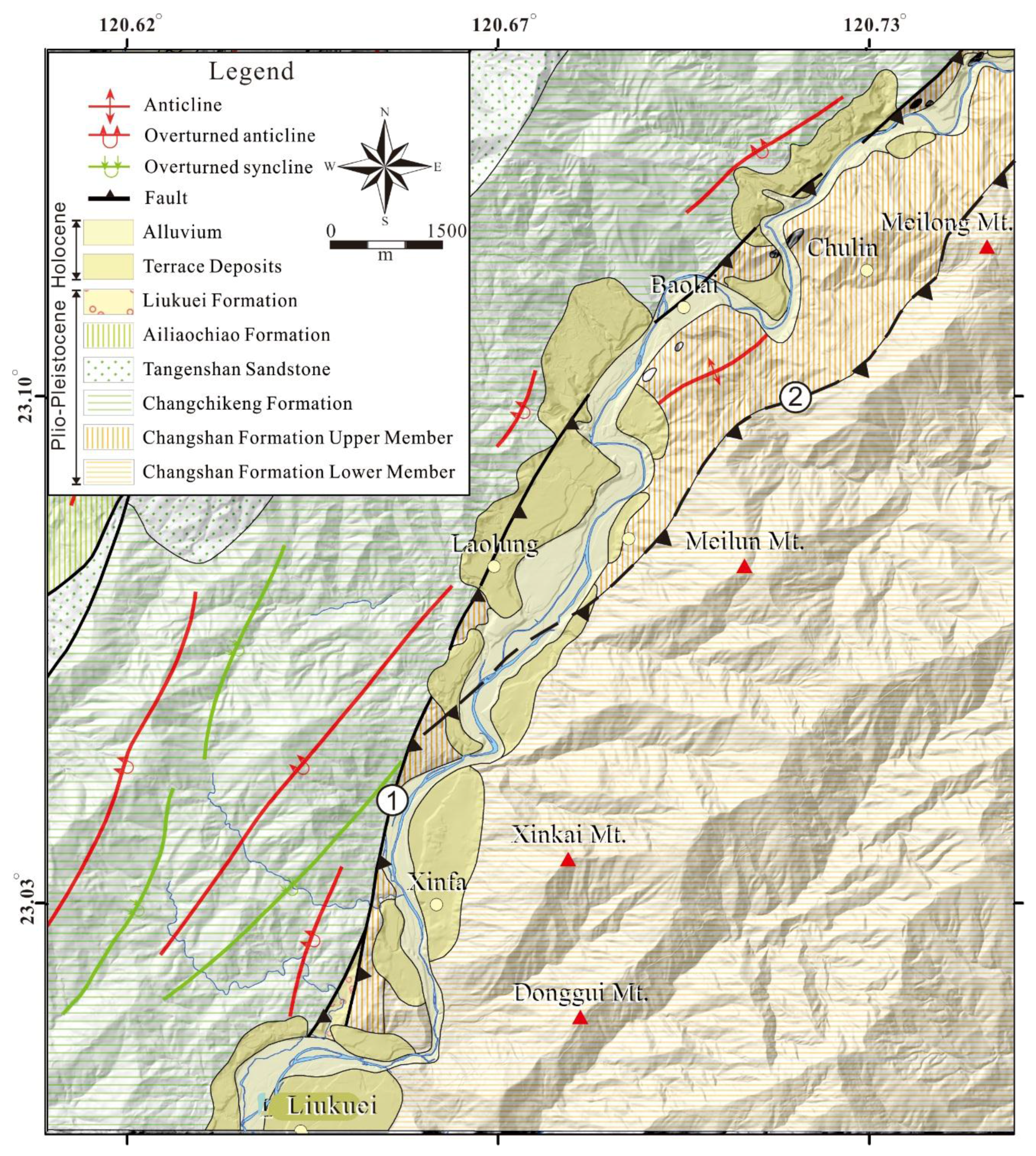Several regions, which are marked by yellow solid lines and stars in Figure 1, constitute the area that was selected for our detailed survey that used aerial photos, field investigations and the LiDAR-derived DEMs. The exposed rocks in the study area include the Miocene Changshan Formation, the Miocene Changchikeng Formation, and Holocene–Pleistocene terrace and alluvium deposits (Figure 2). The Changshan Formation is divided into upper and lower members. The lower member of the Changshan Formation primarily consists of slate, with occasional thin- to thick-bedded metamorphic sandstone. The upper member of the Changshan Formation is composed predominantly of argillites with lenticular metamorphic sandstone. Slumping structures are commonly observed in the upper and lower members of the Changshan Formation. The Changchikeng Formation is a flush-type formation and is highly susceptible for landslides. This formation primarily consists of alternating sandstone, siltstone, and shale. The sandstone and siltstone are light to dark gray in color, exhibit a fine-grained texture and generally range in bed thickness from tens of centimeters to two meters. The Pleistocene–Holocene terrace and alluvium deposits are primarily composed of silts, sands, pebbles and conglomerates.

Figure 1. Location of the study area. (a) Bathymetric and tectonic framework around Taiwan. The black arrows with rates show the current movement of the Philippine Sea plate relative to the Chinese continental margin based on GPS data [28]. The small red frame shows the location of the study area. Geological divisions are marked by I: Coastal Plain, II: Western foothills, III: Hsehshan Range, IV: Central Range, and V: Coastal Range [27]. (b) Orthoimage of the Formosat-2 satellite (2-m resolution/pixels), which shows severe landslides that occurred during the 2009 Typhoon Morakot in the study area.

Figure 1. Location of the study area. (a) Bathymetric and tectonic framework around Taiwan. The black arrows with rates show the current movement of the Philippine Sea plate relative to the Chinese continental margin based on GPS data [28]. The small red frame shows the location of the study area. Geological divisions are marked by I: Coastal Plain, II: Western foothills, III: Hsehshan Range, IV: Central Range, and V: Coastal Range [27]. (b) Orthoimage of the Formosat-2 satellite (2-m resolution/pixels), which shows severe landslides that occurred during the 2009 Typhoon Morakot in the study area.

The Laolung Fault is a major thrust with a left lateral motion component and is located between sedimentary rock and metamorphic rock in southwestern Taiwan [30]. This fault is a northern extension of the Chaochou Fault, which is a “concealed or inferred fault” but has been documented as being an active fault [31,32]. In the selected study area, the Laolung Fault trends NE–SW and dips eastward, with a dip angle within the range of 50°–65°. The faults are primarily underlain by terrace and fluvial deposits, and only a few fault outcrops are exposed (Figure 2). The Meilongshan Fault is an inferred fault and is roughly located along the boundary between the upper and lower Changshan Formation. This fault merges into the Laolung Fault in the Laolung River near Shinfa. No field evidence regarding the existence and the characteristics of the Meilongshan Fault has been previously documented. This fault is primarily inferred from the attitude variations in bedding and cleavage and the lithological contrast between the upper and lower members of the Changshan Formation [33].

Figure 2. Geological map of the study area [34] draped over a relief shading that was generated from a 40-m-resolution Digital Terrain Model. The Laolung Fault is labeled with the number “1”, and the Meilongshan Fault is labeled with the number “2”.

Figure 2. Geological map of the study area [34] draped over a relief shading that was generated from a 40-m-resolution Digital Terrain Model. The Laolung Fault is labeled with the number “1”, and the Meilongshan Fault is labeled with the number “2”.

In the area of the Changshan Formation (Figure 1), the elevation ranges from 245 to 1897 m. The slope distribution, excluding the plains, primarily falls within the range of 20°–45°, with a mean slope of 28°. The area has a typical sub-tropic climate with a mean annual rainfall of approximately 3500 mm. Precipitation primarily occurs from May to September. The weathered topsoil covers exhibit varying thicknesses from tens of centimeters to several meters covering the bedrock geology.

3. Dataset and Methodology

Aerial photos and different visualizations of LiDAR-derived-DEMs, including slope maps, openness with a tinted color slope map, and a 3D RRIM, are employed to identify subtle topographic signatures in the slate area.

3.1. Airborne LiDAR-Derived DEM

A detailed LiDAR dataset that was commissioned by the Central Geological Survey [35] is available for the study area. During the flight, both LiDAR data and 25-cm-resolution aerial photos were obtained using a Leica ALS60 laser scanner equipped with a digital camera; this laser scanner was installed on an airplane that flew at an average altitude of 3000 m above ground level. The digital aerial photos include elementary position information that was derived from the on-board IMU, which was ortho-rectified with the LiDAR data from the same flight. The flying speed was approximately 100 knots, the maximum field of view (FOV) was 40°, and the pulse rate was 114.6 kHz. The survey average point density was specified to be greater than 2 points/m² for the study areas and 1 point/m² for bare ground. LiDAR point measurements were filtered into returns from vegetation and bare ground using the Terrascan™ software’s classification routines and algorithms. The vertical accuracy, which was evaluated by a direct comparison between the LiDAR and ground DGPS elevation points, was estimated to be less than 0.3 m in flat areas, which is an acceptable value for LiDAR analyses in the field of geomorphology [36].

The processed airborne LiDAR data were further interpolated to derive a grid of digital surface models (DSMs) and DEMs with vegetation and buildings removed. The LiDAR bare ground data set was used to generate a 1-m-resolution DEM using the natural neighbor interpolator, which has proven to be useful for geomorphic analysis in previous studies [37].

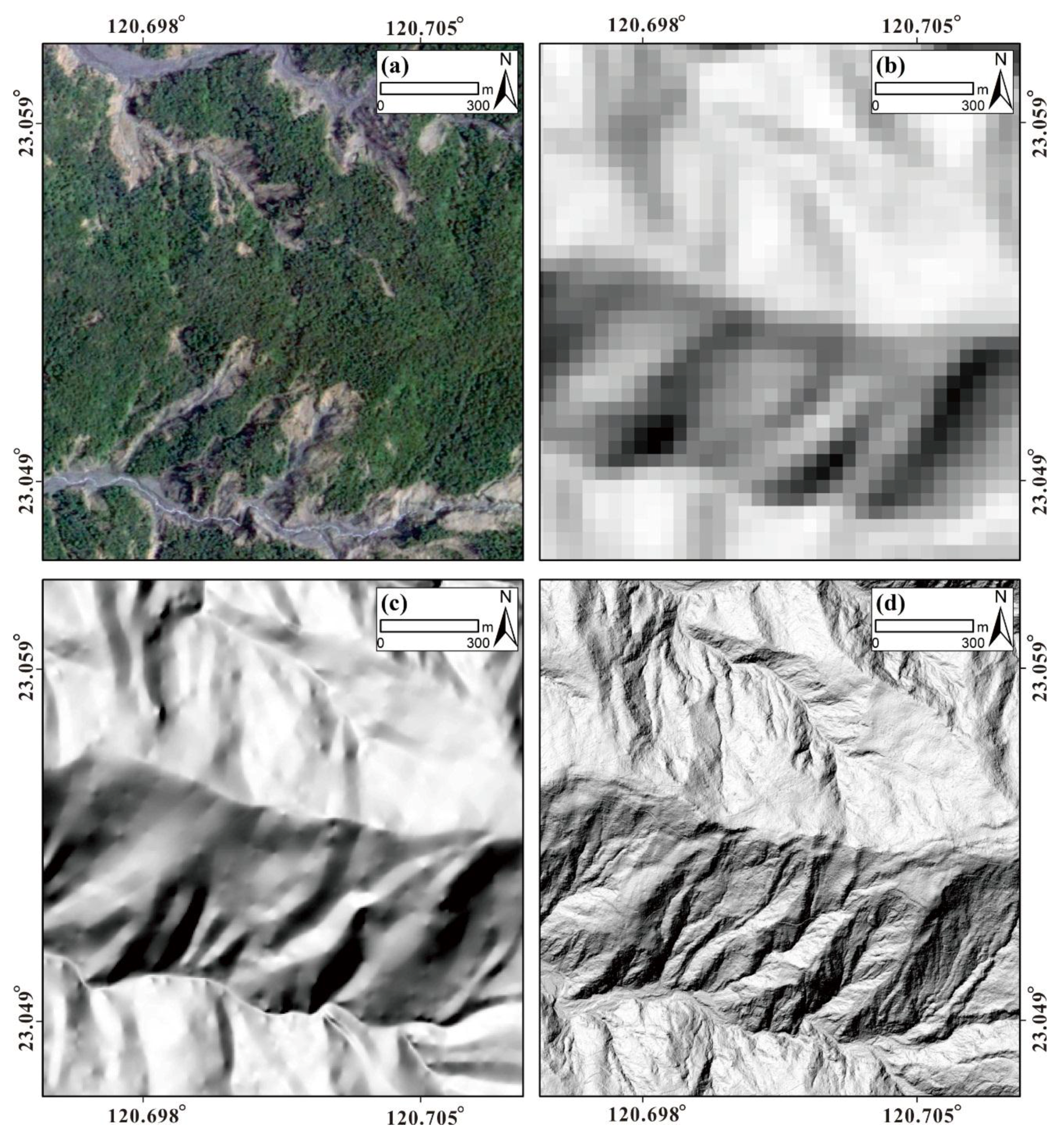
To compare the visibility of images with different resolutions to detect subtle topographic signatures, DEMs with different resolutions are shown in Figure 3. A 25-cm-resolution aerial photo that was obtained on the same flight during which the LiDAR data were obtained is shown in Figure 3. In the aerial photo, nearly no topographic signature, with the exception of landslide scars, can be identified because of heavy vegetation. However, bare ground that was created by landslides provides an excellent opportunity for field investigations of tectonic-geomorphic phenomena such as fault scarps, tilting terraces, river channel offsets and abandoned channels. Figure 3b shows a 40-m-resolution DTM that was generated through traditional photogrammetric techniques and corresponds to the most popular data that have been used in topographic and geological analyses in Taiwan. Subtle topographic signatures cannot be observed in the image because of its poor resolution. An image from a 5-m-resolution DTM, which was also derived using photogrammetric techniques, is shown in Figure 3c. Large and significant tectonic-geomorphic structures can be identified in the 5-m DTM, but subtle structures cannot be distinguished. Figure 3d shows an image from a 1-m-resolution LiDAR-derived DEM that was used in this study. Compared to previous images, LiDAR-derived high-resolution DEMs provide detailed real bare earth topography and can effectively detect subtle topographic signatures that cannot be recognized by simply using aerial photographs or satellite images.

Figure 3. An aerial photo and shaded relief maps derived from different-resolution DEMs of a selected area that is marked in Figure 1. (a) Aerial orthophoto with a 25-cm-resolution; (b) 40-m DTM; (c) 5-m-resolution DEM; (d) 1-m-resolution LiDAR-derived DEMs alter filtering buildings and vegetation. The illumination direction of the shaded relief map was set with an azimuth of 315° and an inclination of 45°.

Figure 3. An aerial photo and shaded relief maps derived from different-resolution DEMs of a selected area that is marked in Figure 1. (a) Aerial orthophoto with a 25-cm-resolution; (b) 40-m DTM; (c) 5-m-resolution DEM; (d) 1-m-resolution LiDAR-derived DEMs alter filtering buildings and vegetation. The illumination direction of the shaded relief map was set with an azimuth of 315° and an inclination of 45°.

3.2. Openness Analysis

High-resolution LiDAR DEMs are generally examined on a shaded relief map and/or a slope map [23]. The shaded relief map is widely used because it resembles what we see in the real world. However, it has the significant disadvantage that the appearance of the image completely changes depending on the direction of incident illumination. The slope map is independent of the illumination but is quite different from our visual perception and cannot distinguish convexity and concavity. However, high-resolution three-dimensional topographic data potentially holds useful information that cannot be expressed by an ordinal visualization method. In contrast to traditional sunshine shadow images, an openness analysis of a LiDAR image can remove the effects of luminance during image interpretation. An openness technique expressing the degree of dominance or enclosure of a location on an irregular surface was developed by Yokoyama et al. [38], and this technique calculates an angular measure of the relationship between surface relief and horizontal distance [39,40]. It uses the horizontal surface distance and elevation-related angle to compute the slope information of an irregular terrain surface at different positions, and the results can be used to identify the topographic features of the area. This method calculates the zenith and nadir angles at equally spaced locations in eight azimuth directions from the line of sight of the terrain (Figure 4a). The openness analysis yields the maximum and minimum values for eight different azimuth directions from point A (Azimuth direction D = 0°, 45°, 90°, 135°, 180°, 225°, 270°, and 315°) at a radius of L, and the slope values ${}_D\beta _L$ and ${}_D\delta _L$ for the different azimuth angles are then calculated. In addition, using Equations (1) and (2), the zenith angle (${}_D\beta _L$) and nadir angle (${}_D\delta _L$) can be calculated.

$${}_D\mathrm{\Phi }_L=90°-{}_D\beta _L$$

(1)

$${}_D\mathrm{\Psi }_L=90°-{}_D\delta _L$$

(2)

Finally, the average angle for each direction is calculated using Equations (3) and (4) to obtain positive (${\mathrm{\Phi }}_L$) and negative (${\mathrm{\Psi }}_L$) openness values, which represent ridges and valleys in the topography, respectively (Figure 4b,c). The openness parameter is designated “positive” or “negative” in the sense that has been used to express terrain-slope curvature [41]. A positive openness is convex-upward and refers to a calculation using zenith angles, whereas negative openness is concave-upward and refers to an evaluation with nadir angles [38]. The conceptual model of the openness analysis is represented by an I value, which is calculated using Equation (5). Figure 4d shows an openness map that more accurately and simultaneously represents topographic ridges and valleys compared with Figure 4b,c. The openness technique efficiently eliminates incident light direction dependency, such as in shaded relief images. Convex topography is represented by a high positive openness value, whereas concave topography is characterized by a low positive openness value. (Figure 4b).

$${\mathrm{\Phi }}_L=\left({}_0\mathrm{\Phi }_L+{}_{45}\mathrm{\Phi }_L+\mathrm{\dots }+{}_{315}\mathrm{\Phi }_L\right)/8$$

(3)

$${\mathrm{\Psi }}_L=\left({}_0\mathrm{\Psi }_L+{}_{45}\mathrm{\Psi }_L+\mathrm{\dots }+{}_{315}\mathrm{\Psi }_L\right)/8$$

(4)

$$I=\frac{\left({\mathrm{\Phi }}_L-{\mathrm{\Psi }}_L\right)}{2}$$

(5)

Figure 4. Openness techniques and images obtained. (a) Concept diagram showing to the calculation of the parameters (modified from [26,38]). An example selected from the area shown in Figure 1 to illustrate the characteristics of (b) positive openness, (c) negative openness, and (d) openness images. The openness value was computed from 1-m-resoultion LiDAR-derived DEMs.

Figure 4. Openness techniques and images obtained. (a) Concept diagram showing to the calculation of the parameters (modified from [26,38]). An example selected from the area shown in Figure 1 to illustrate the characteristics of (b) positive openness, (c) negative openness, and (d) openness images. The openness value was computed from 1-m-resoultion LiDAR-derived DEMs.

The results of the openness analysis highlight positions with strong angular variations in their terrain features, such as crests, ridges, gullies and valleys. In addition, this method overcomes the shortcomings of sunshine shadows, which are caused by variations in the light source direction during mapping.

3.3. RRIM and 3D Visualization

RRIM is a new 3D LiDAR visualization approach that was proposed by Chiba et al. [25,26]. An RRIM is a multi-layered illumination-free image that can be used to simultaneously visualize topographic slopes, concavities and convexities. The basic concept of an RRIM is to multiply three landform element layers: topographic slopes, positive openness and negative openness. An RRIM is generated using an overlay of a red-colored slope map on the I-value map. The color red is used to describe the slope angle because it has been empirically demonstrated to provide the richest tone for human eyes. This overlay highlights the 3D topography on a single image, where the I-value performs an illumination role and the saturation of red describes the steepness of the topography. The results that are obtained from an RRIM with 3D visualization and a geographic information system (GIS) are merged with a new topographic parameter. In addition to enabling illumination-independent 3D visualization, RRIMs are sensitive to subtle topographic changes. Figure 4a shows how RRIMs can be tuned to express various scales of topography in detail by adjusting the zenith and nadir angles along the compass directions within the radial limit (L). These advantages can maximize the visibility of subtle tectonic-geomorphic structures in high-resolution LiDAR-derived DEMs.

4. Results

Three areas, which are marked with yellow stars in Figure 1, were selected for a detailed investigation that used aerial photos and LiDAR-derived DEMs. In addition, field investigations were performed to confirm the results of the image interpretations.

4.1. Interpretation of Fault Zone

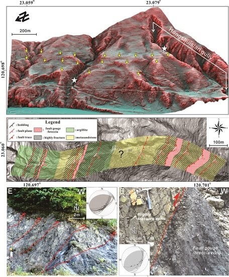
The Meilongshan Fault is a NE–SW-trending fault that extends for approximately 15 km [33] and is roughly located along the boundary between the upper and lower Changshan Formation (Figure 2). The Meilongshan Fault is a concealed fault and is primarily inferred from the lithological contrast and variations in bedding and cleavage attitude. No specific outcrop has been documented to characterize this fault. In this study, a specific area (Figure 1 and Figure 5) near Meilun Mountain that covers 0.85 km² was selected for a detailed investigation of the tectonic geomorphic features and to illustrate the existence and characteristics of the Meilongshan Fault.

A 25-cm-resolution aerial photo that was captured while the LiDAR-DEM data were captured in 2010 shows that the study area is covered by heavy vegetation (Figure 5a). A landslide that was induced by Typhoon Morakot in 2009 stripped off some vegetation, thus providing excellent exposures for a detailed field investigation. Although covered by heavy vegetation, a general NE–SW-trending lineament that passes through the central part of the study area can be observed, particularly compared with Figure 5b. The study area is interpreted to be covered by colluvium deposits based on certain boulders that were observed in the slope image of the LiDAR data (Figure 5b). Five E–W-trending gullies that flow parallel to the slope direction can be identified in the slope image. However, only the middle gully can be observed in the aerial photo (Figure 5a). In addition, two NE–SW-trending linear scarps can be observed in the image. Because argillite is the predominant exposed lithology in the study area, linear scarps that were caused by the differential erosion of the lithology are excluded. The lower scarp has been modified by landslides and thus does not look very straight. However, the higher scarp is relatively straight, indicating that a landslide likely did not form the croissant-shaped scarp. In addition, a field investigation confirmed that at least a 750-m-wide deformation zone developed, which implies that the scarp is of tectonic origin. A 35-m and 28-m vertical topographic relief is measured from the DEM along the slope direction for the upper and lower fault scarps, respectively.

Significant changes in the flowing path of the gullies when they pass the upper linear scarp are also observed in the slope map. We detected several gullies (gullies 1, 3 and 5) that exhibit approximately 40 m of left lateral offset, which conforms to the fault slip measurement. In addition, several croissant-shaped scarps that represent the crown scarps of active landslides can be observed in the lower part of the image. Figure 5c shows a map that combines a slope map that is tinted in red-green and the openness metric in gray. In this map, red represents areas with a large slope gradient, and green represents areas with small slope gradients. Compared to the slope image (Figure 5b), areas with steep slopes, which are shown in red and include steep slopes next to gullies, landslide scarps, and fault scarps, can be more easily identified in Figure 5c. In contrast to gullies 1, 3, and 5, which were identified in the slope image, five gullies that were derived from a hydrology analysis with Arc GIS are obtained in Figure 5c. Two newly identified gullies, 2 and 4, exhibit a subtle valley geometry without significant down cutting of the slope. Gullies 2 and 4 also exhibit changes in their flow path when passing through the linear fault scarps. This observation highlights that the geomorphic and surface process conditions in this area are sufficiently dynamic and morphologically susceptible to new gully formation. A 3D perspective of the RRIM image provides a virtual reality of the study area (Figure 5d) and allows the imagery to be displayed with different orientations and inclinations. Compared to previous images, fault scarps and gullies can be more clearly observed in the 3D perspective. The attitude of the fault plane at approximately N20°E/70°E can be calculated from the DEM. In addition, the third fault scarp, which is located near the foothill of the slope, can be identified, although parts of it have been eroded by landslides.

A field investigation along the gullies was performed to verify the results of our interpretations. In the field investigation, argillites with thin bed metamorphosed sandstones are the dominant exposed lithologies. The fault zone, which primarily consists of a series of thrusts with fault gouge and breccia, extends at least a 750-m-wide deformation zone (Figure 5e) from the lowest fault scarp to the point approximately 50 m beyond the highest scarp. Four fault gouge and/or fault breccia zones are recognized with the 750-m deformation zone. The thickness of each gouge and/or fault breccia zone from west to east is 6.9-m, 7.3-m, 24.2-m and 38.6-m. The rocks near these fault gouge zones are highly fractured. Field measurements of fault slip in these zones are consistent, showing thrusting with a minor component of left lateral motion. Photos of two fault outcrops that are located near the lowest and highest scarps are shown in Figure 5f. The outcrop near the lowest fault scarp exhibits several eastern dipping thrusts, which can be observed as a dark gray band in the photograph shown on the left-hand side of Figure 5f. The outcrop near the upper fault scarp is located at the boundary of 24.2-m-thick fault gouge and/or fault breccia zone. Highly fractured metamorphic sandstone resting on thick fault breccia are depicted in the photograph on the right-hand side of Figure 5f. Fault slip data measured at outcrops were also plotted using Schmidt’s (equal area) lower hemisphere projection. The results indicate that most of faults are west vergent, high-angle, and reverse faults with a minor component of left lateral movement.

Figure 5. Aerial and field photographs and LiDAR imagers of a selected area in Figure 1. These images illustrate the characteristics of faults in outcrops. (a) Color aerial orthophoto that illustrates that most of the tectonic geomorphic features are obscured by dense forest cover. (b) Bare earth LiDAR slope imagery that shows NE–SW-trending linear low-relief fault scarps (marked with dashed red lines) on the colluvium deposits. Salient points (marked with black circles) in the slope imagery are interpreted as boulders on the slope. The white dashed lines are marked to illustrate the offset of gullies 1, 3 and 5. (c) Openness with a tint slope map that enhances the locations of linear fault scarps. The color bar represents the degree of the slope angle. (d) A 3D perspective of the RRIM map shows three linear fault scarps that are located within a 750-m-wide fault zone. The traces of the fault scarps, which are identified by subtle tectonic-geomorphic features, are indicated by yellow arrows. (e) Results of the traverse geological mapping along the gully in Figure 5d. (f) Field photographs showing fault outcrops that are located along the upper (right photo) and lower (left photo) boundaries. Fault slip data that were measured at each outcrop are also illustrated by using Schmidt’s (equal area) lower hemisphere projection. Fault planes are drawn as large circles, arrows indicate the slip of the hanging wall in the direction of the arrowhead, and head styles express the degree of confidence of the slip-sense determination.

Figure 5. Aerial and field photographs and LiDAR imagers of a selected area in Figure 1. These images illustrate the characteristics of faults in outcrops. (a) Color aerial orthophoto that illustrates that most of the tectonic geomorphic features are obscured by dense forest cover. (b) Bare earth LiDAR slope imagery that shows NE–SW-trending linear low-relief fault scarps (marked with dashed red lines) on the colluvium deposits. Salient points (marked with black circles) in the slope imagery are interpreted as boulders on the slope. The white dashed lines are marked to illustrate the offset of gullies 1, 3 and 5. (c) Openness with a tint slope map that enhances the locations of linear fault scarps. The color bar represents the degree of the slope angle. (d) A 3D perspective of the RRIM map shows three linear fault scarps that are located within a 750-m-wide fault zone. The traces of the fault scarps, which are identified by subtle tectonic-geomorphic features, are indicated by yellow arrows. (e) Results of the traverse geological mapping along the gully in Figure 5d. (f) Field photographs showing fault outcrops that are located along the upper (right photo) and lower (left photo) boundaries. Fault slip data that were measured at each outcrop are also illustrated by using Schmidt’s (equal area) lower hemisphere projection. Fault planes are drawn as large circles, arrows indicate the slip of the hanging wall in the direction of the arrowhead, and head styles express the degree of confidence of the slip-sense determination.

4.2. Interpretation of Regional Cleavage Attitude

Structural fabrics, such as cleavage in slate, are often difficult to perceive in forested metamorphic terrain because of vegetation, sediment cover, low topographic relief, and the overprinting of structural lineaments. However, these structural elements can be observed using airborne LiDAR DEMs [42]. Although not all lineaments that are identified in LiDAR DEMs can be correlated to mapped structures, our analysis demonstrates that LiDAR data provide valuable information that can be used to accurately determine the regional cleavage attitude in a slate terrain. Several N–S-trending lineaments and landslides are observed. The slope image (Figure 6b) shows an area located in the central part of the image that exhibits parallel, planar, triangular faces, which are interpreted as the sheeting texture that formed from the cleavage of slate. These triangular faces likely formed from weathered debris material sliding along cleavage, resulting in the thick slabs shown in Figure 6b compared with the penetrative cleavage. Figure 6c shows a slope map that is tinted in red-green and overlain by the openness metric shown in Figure 6b, which is illustrated in gray. Symmetric erosion gullies that are distributed along the northern and southern flanks of the main ridge can be easily discerned in Figure 6c. Dark red lineaments in the image also clearly define several yellow-green triangular faces. These triangular faces represent planar geological structures and are interpreted as cleavage in slate (Figure 6c). A 3D perspective of the RRIM image is shown in Figure 6d. Compared to previous images, the triangular faces that were formed by cleavage can be more clearly observed in the 3D perspective. The regional cleavage attitude measured from the DEM is N–S/75°W.

Figure 6. Aerial and field photos and LiDAR-derived imageries of a selected area in Figure 1, which illustrate the cleavage characteristics. (a) Color aerial orthophoto that shows several landslides and N–S-trending lineaments. (b) Triangle faces that represent cleavage that is bounded by N–S-trending lineaments can be identified in the slope image. (c) The N–S-trending ridges and triangle faces are enhanced in the openness with a tint color slope image. The color bar represents the degree of the slope angle. (d) Cleavage-formed ridges and triangle faces are clearly observed in the 3D perspective of the RRIM map. (e) The outcrop shows the buckling of cleavage in slate. (f) A schematic sketch that illustrates how the triangle face reflects the cleavage. The field measurements of the cleavage attitudes are plotted by lower-hemisphere equal-area projection. The large circles are cleavage planes, and the pole represents the lineation attitude.

Figure 6. Aerial and field photos and LiDAR-derived imageries of a selected area in Figure 1, which illustrate the cleavage characteristics. (a) Color aerial orthophoto that shows several landslides and N–S-trending lineaments. (b) Triangle faces that represent cleavage that is bounded by N–S-trending lineaments can be identified in the slope image. (c) The N–S-trending ridges and triangle faces are enhanced in the openness with a tint color slope image. The color bar represents the degree of the slope angle. (d) Cleavage-formed ridges and triangle faces are clearly observed in the 3D perspective of the RRIM map. (e) The outcrop shows the buckling of cleavage in slate. (f) A schematic sketch that illustrates how the triangle face reflects the cleavage. The field measurements of the cleavage attitudes are plotted by lower-hemisphere equal-area projection. The large circles are cleavage planes, and the pole represents the lineation attitude.

The field investigation confirmed that the triangular faces that were observed in the LiDAR image are cleavages in slates. However, the field measurements of the cleavage attitudes fall over a wide range (Figure 6e). The strike of the cleavage is from N30°E to N20°W, dipping to the west with a dip angle of 30°–80°. The variation in the cleavage attitude that was measured in the field is primarily caused by the creeping of gravitation. The image of the outcrop in Figure 6e shows the buckling of slate and illustrates why the cleavage attitude that was measured in the field exhibits large variability. In the slate terrain, creeping from gravitation is sufficiently common such that the attitude at the outcrops typically cannot properly represent the regional cleavage attitude. However, the triangular faces that were identified in the LiDAR images exhibit consistent orientation and extend several hundreds of meters. Therefore, the attitude that was measured by the LiDAR DEM accurately represents the regional cleavage attitude in the study area (Figure 6f).

4.3. Interpretation of Deep-Seated Landslides

Deep-seated gravitational slope deformations (DSGSDs) are generally linked to high relief mountain environments and are voluminous, short-traveling and slow-moving failures [43,44,45,46,47]. DSGSDs occasionally transform into fast moving and catastrophic, long run-out rockslides, which might pose a significant hazard to areas that are situated large distances from source zones. Conventional DSGSD mapping focuses on the evident morpho-structural features that accompany mass slope movement [48,49], such as the main escarpment, crown scarps, trenches, double ridges and deformed foothill deposits. These landslide signatures are also the major indicators that are used for field investigations and aerial photo interpretations. Chigira et al. [24] illustrated that some large, catastrophic landslides that were induced by Typhoon Talas in 2011 were preceded by deep-seated gravitational slope deformation. The series of deep-seated landslides identified from the LiDAR DEM are documented in the eastern part of the study area [50] (see Figure 1). A specific study area (Figure 1 and Figure 7) was selected to illustrate the usefulness of employing LiDAR-derived-DEM and related visualization techniques to detect these deep-seated landslides scars.

Various shallow landslides can be observed in the aerial photos in Figure 7a. In addition, several nearby crown scarps that are roughly parallel to the main ridge of the catchment can be identified, and the boundary of the deep-seated landslide can be approximately determined. In the slope image that was generated using the LiDAR data (Figure 7b), several N–S-trending, NE–SW-trending, and N–W-trending linear features distributed near the ridge are more clearly shown compared with the aerial photo. The N–S-trending linear features are relatively straight, and their orientations are consistent with the regional cleavage orientation. Thus, these features are interpreted as scarps that formed by slipping along cleavage planes. The E–W- and NE–SW-trending linear features are composed of several small croissant -shaped scarps and are interpreted as crown scarps that formed by slipping along the slope direction.

The shallow landslide area that is represented by an area with a rugged surface in the slope image is substantially larger than that observed in the aerial photo. Various croissant-shaped crown scarps are also observed in the upper portion of the slope. In the image that combines the slope map, which is tinted in red-green and the openness metric in gray (Figure 7c), linear crown scarps that are located near the ridge and croissant-shaped scarps that are located in the middle of the slope can be easily identified based on the distribution of dark red lines. Trenches that are located between small ridges, which are areas indicated in green, are also easily observed. A 3D perspective of the RRIM image provides a virtual reality of this study area (Figure 7d). Compared to the previously mentioned images, small ridges that are represented by red lines and are parallel to the main ridge of the catchment can be easily identified. Typical double ridges and trenches can be identified in the topographic profile in Figure 7d.

Figure 7. Aerial and field photos and LiDAR images of a selected area in Figure 1. These images illustrate the characteristics of a deep-seated landslide. (a) A color aerial image that shows a selected deep-seated landslide in the marked area in Figure 1. (b) Crown scarps of the deep-seated landslide are easily observed in the LiDAR image. (c) Crown scarps of the deep-seated landslide are enhanced in the openness with a tint-colored slope image. The color bar represents the degree of the slope angle. (d) A 3D perspective of the RRIM map that shows the topographic characteristics of the deep-seated landslide. The yellow arrows indicate the locations of crown scarps. The topographic profile exhibits trenches and double ridge topography. (e) Two images that were obtained at the locations shown in (d). (f) A crown scarp with a displacement of approximately 50 cm is shown in the upper photograph. The lower photo exhibits a crown scarp with a displacement of more than 100 cm. Buckling of the argillite is also seen in the lower photograph.

Figure 7. Aerial and field photos and LiDAR images of a selected area in Figure 1. These images illustrate the characteristics of a deep-seated landslide. (a) A color aerial image that shows a selected deep-seated landslide in the marked area in Figure 1. (b) Crown scarps of the deep-seated landslide are easily observed in the LiDAR image. (c) Crown scarps of the deep-seated landslide are enhanced in the openness with a tint-colored slope image. The color bar represents the degree of the slope angle. (d) A 3D perspective of the RRIM map that shows the topographic characteristics of the deep-seated landslide. The yellow arrows indicate the locations of crown scarps. The topographic profile exhibits trenches and double ridge topography. (e) Two images that were obtained at the locations shown in (d). (f) A crown scarp with a displacement of approximately 50 cm is shown in the upper photograph. The lower photo exhibits a crown scarp with a displacement of more than 100 cm. Buckling of the argillite is also seen in the lower photograph.

The field investigation confirmed the interpretations of the aforementioned photographs. Shallow landslides are easily recognized in the field. These mainly occurred in the lower part of the hill slope. The field measurement of the cleavage attitude mainly falls within the range of N-N20°E/70°–80°W, which is close to the N–S-trending linear scarps identified (Figure 7b,c). In the A-A’ topographic profile cutting perpendicular to the NE–SW-trending scarps, as shown in Figure 7d, typical double ridges and trenches can be identified. In addition, most of the scarps identified in LiDAR images can be recognized if they are accessible. A crown scarp with a displacement of approximately 50 cm is shown in the upper image in Figure 7e. Furthermore, the buckling of argillite, which is one of the dominant deformation mechanisms in gravitational deformation, is also observed at a crown scarp.

5. Discussion

Bare earth airborne LiDAR imagery have revolutionized geomorphic and fault mapping in dense forest areas, where it may otherwise be extremely difficult or impossible to reinterpret landforms using traditional approaches [51,52]. Several different applications of LiDAR have been demonstrated in the study of active faults, such as tracing and mapping active faults [18], tectonic-geomorphic analysis, the extraction of the detailed geometry and kinematics of fault zones [53], the extraction of throw-rates along postglacial scarps [54], and mapping the deformation processes [55]. Additionally, LiDAR DEM has also been successfully applied for the detection and characterization of deep-seated landslides [43].

This study uses LiDAR-derived DEMs and effectively combines data using different visualization approaches to characterize subtle tectonic-geomorphologic signatures in dense forest areas. The results of the study show that fault scarps, crown scarps of deep-seated landslides, and subtle ridges that are formed by cleavages can be discerned in grayscale slope images, which are useful for identifying scarps that are steeper than the surrounding slopes. In the openness with a tinted slope image, positive openness values indicate the aforementioned features, and negative values indicate canyons, valleys, and gullies. Therefore, the fault scarps and gullies in the study area were accurately represented using the openness technique. In addition, the crown escarpment of deep-seated landslides and subtle ridges that represent the cleavages of slate in the study area can also be observed in the openness image. A 3D perspective of the RRIM allows us to investigate images that are rotated to different orientations and inclinations. If the fault movement is minor or is rapidly eliminated or modified by erosion, then subtle tectonic geomorphic signatures are also difficult to identify in a plane view. Therefore, a 3D perspective image is the best visualization approach for interpreting geological structures.

In this study, we successfully applied airborne LiDAR surveying techniques to illustrate how to analyze and visualize areas in which active faults are difficult to traced due to dense vegetation cover and high erosion rates. The Meilongshan Fault, which was previously categorized as an inferred fault, was effectively defined in the investigated area using different LiDAR visualization images. The fault on the surface is distributed over a 750-m-wide deformation zone and exhibits three distinct, NE-trending scarps. A series of NE–SW-trending thrusts with fault gouges and breccia within the fault zone can be identified in the field. The faulting that produced the newly revealed scarp most likely occurred in association with a left-lateral strike-slip. Although none of the existing dating information confirms that the fault is active, clear fault scarps are preserved in the area with violent surface geological processes, indicating that the last fault motion likely occurred recently. Another important observation from the LiDAR images is the gullies that were investigated using the openness metric in the slope image. Gullies that flow through the fault zone change their paths, which also implies that the Meilongshan Fault is an active fault.

Active structures provide various advantages in multiple aspects of seismic hazard mitigation for the long-term forecasting of surface deformation during significant earthquakes and for obtaining important information on deep fault structures at depth [56,57]. Using LiDAR data and the proposed visualization approaches, this study illustrates how fault traces can be identified and how the outcrop locations of a significant and unknown thrust in a high-vegetation area with a high erosion rate can be defined. Because it is more difficult to study thrust faults and identify their traces [58], the approaches used in this study can be applied to other compression tectonic terrains to aid the mapping of geological structures such as thrusts and cleavage. Because fault scarps are easily identified in 1-m resolution LiDAR DEMs, quantitative deformation data can be extracted in a further study through the construction of topographic profiles measured perpendicular to the trace of the scarp if it offsets sediments of known age [59]. Furthermore, LiDAR surveying techniques can also effectively assist future paleoseismological studies and trenching because the fault plane/zone can now be located with accuracy, even in a densely forested environment.

6. Conclusions

High-resolution LiDAR-derived DEMs provide detailed tectonic geomorphic signatures in bare ground. In this study, we successfully used 1-m-resolution LiDAR data and applied various visualization approaches, including slope images, openness visualizations, RRIMs, and 3D perspective images, to illustrate how to analyze and visualize an area in which active faults, cleavages, and deep-seated landslides are difficult to identify due to dense vegetation and high erosion rates. An inferred fault, the Meilongshan Fault, whose characteristics were previously undocumented, was identified as a NE–SW-trending, eastern-dipping high-angle thrust with a 750-m-wide fault zone. Different visualization approaches were compared using three examples to illustrate the advantages and disadvantages of each approach. To interpret deep-seated landslides and geological structures, such as cleavages of slate and faults, slope images with openness analysis can be used to identify ridges, fault scarps, and crown scarps, therefore providing a substantial benefit to the identification of such phenomena. The best opportunity for observation was provided by 3D perspective images with RRIMs because the images could be viewed at any orientation and inclination. However, the interpreted results, even if obtained using a l-m-resolution DEM, must still be confirmed by field observations.

References

- Wallace, R.E. Active Tectonics. Studies in Geophysics; The National Academies Press: Washington, DC, USA, 1986; pp. 136–147. [Google Scholar]
- Papanikolaοu, I.D.; van Balen, R.; Silva, P.G.; Reicherter, K. Geomorphology of Active Faulting and seismic hazard assessment: New tools and future challenges. Geomorphology 2015, 237, 1–13. [Google Scholar] [CrossRef]
- Guzzetti, F.; Cardinali, M.; Reichenbach, P.; Cipolla, F.; Sebastiani, C.; Galli, M.; Salvati, P. Landslides triggered by the 23 November 2000 rainfall event in the Imperia Province, Western Liguria, Italy. Eng. Geol. 2004, 73, 229–245. [Google Scholar] [CrossRef]
- Prokesova, R.; Kardos, M.; Medvedova, A. Landslide dynamics from high-resolution aerial photographys: A case study from the Western Carpathians, Slovakia. Geomorphology 2010, 115, 90–101. [Google Scholar] [CrossRef]
- Mondini, A.C.; Chang, K.T.; Yin, H.Y. Combining multiple change detection indices for mapping landslides triggered by typhoons. Geomorphology 2011, 134, 440–451. [Google Scholar] [CrossRef]
- Bovenga, F.; Wasowski, J.; Nitti, D.O.; Nutricato, R.; Chiaradia, M.T. Using COSMO/SkyMed X-band and ENVISAT C-band SAR interferometry for landslides analysis. Remote Sens. Environ. 2012, 119, 272–285. [Google Scholar] [CrossRef]
- Wehr, A.; Lohr, U. Airborne laser scanning—An introduction and overview. ISPRS J. Photogramm. Remote Sens. 1999, 54, 68–82. [Google Scholar] [CrossRef]
- Tarolli, P.; Arrowsmith, J.R.; Vivoni, E.R. Understanding earth surface processes from remotely sensed digital terrain models. Geomorphology 2009, 113, 1–3. [Google Scholar] [CrossRef]
- Carrara, A.; Cardinali, M.; Guzzetti, F. Uncertainty in assessing landslide hazard and risk. ITC J. 1992, 2, 172–183. [Google Scholar]
- Ardizzone, F.; Cardinali, M.; Carrara, A.; Guzzetti, F.; Reichenbach, P. Impact of mapping errors on the reliability of landslide hazard maps. Nat. Hazards Earth Syst. Sci. 2002, 2, 3–14. [Google Scholar] [CrossRef]
- McKean, J.; Roering, J. Objective landslide detection and surface morphology mapping using high-resolution airborne laser altimetry. Geomorphology 2004, 57, 331–351. [Google Scholar] [CrossRef]
- Hunter, L.E.; Howle, J.F.; Rose, R.S.; Bawden, G.W. LiDAR-assisted identification of an active fault near truckee, California. Bull. Seismol. Soc. Am. 2011, 101, 1162–1181. [Google Scholar] [CrossRef]
- Kondo, H.; Toda, S.; Okumura, K.; Takada, K.; Chiba, T. A fault scarp in an urban area identified by LiDAR survey: A Case study on the Itoigawa–Shizuoka Tectonic Line, central Japan. Geomorphology 2008, 101, 731–739. [Google Scholar] [CrossRef]
- Arrowsmith, J.R.; Zielke, O. Tectonic geomorphology of the San Andreas Fault zone from high resolution topography: An example from the Cholame segment. Geomorphology 2009, 113, 70–81. [Google Scholar] [CrossRef]
- Wechsler, N.; Rockwell, T.K.; Ben-Zion, Y. Application of high resolution DEM data to detect rock damage from geomorphic signals along the central San Jacinto Fault. Geomorphology 2009, 113, 82–96. [Google Scholar] [CrossRef]
- Hilley, G.E.; DeLong, S.; Prentice, C.; Blisniuk, K.; Arrowsmith, J.R. Morphologic dating of fault scarps using Airborne Laser Swath Mapping (ALSM) data. Geophys. Res. Lett. 2010, 37, L04301. [Google Scholar] [CrossRef]
- Tarolli, P. High-resolution topography for understanding Earth surface processes: Opportunities and challenges. Geomorphology 2014, 216, 295–312. [Google Scholar] [CrossRef]
- Cunnungham, D.; Grebby, S.; Tansey, K.; Gosar, A.; Kastelic, V. Application of airborne LiDAR to mapping seismogenic faults in forested mountainous terrain, southeastern Alps, Slovenia. Geophys. Res. Lett. 2006, 33. [Google Scholar] [CrossRef]
- Jaboyedoff, M.; Oppikofer, T.; Abellán, A.; Derron, M.H.; Loye, A.; Metzger, R.; Pedrazzini, A. Use of LIDAR in landslide investigations: A review. Nat. Hazards 2010, 61, 5–28. [Google Scholar] [CrossRef]
- Kagamihara, K.; Hasegawa, S.; Nonomura, A.; Uchida, J. Hazard mapping of earthquake-induced deep-seated catastrophic landslides for different scenario earthquakes by Using LiDAR DEM and airborne resistivity data. Int. J. Landslide Environ. 2013, 1, 37–38. [Google Scholar]
- Zachariasen, J. Detail mapping of the northern San Andreas Fault using LiDAR imagery. In Final Technical Report National Earthquake Hazards Reduction Program; U.S. Geological Survey: Reston, VT, USA, 2008; p. 47. [Google Scholar]
- Chan, Y.C.; Chen, Y.G.; Shih, T.Y.; Huang, C. Characterizing the Hsincheng active fault in northern Taiwan using airborne lidar data: Detailed geomorphic features and their structural implications. J. Asian Earth Sci. 2007, 31, 303–316. [Google Scholar] [CrossRef]
- Lin, Z.; Kaneda, H.; Mukoyama, S.; Asada, N.; Chiba, T. Detection of subtle tectonic–geomorphic features in densely forested mountains by very high-resolution airborne LiDAR survey. Geomorphology 2013, 182, 104–115. [Google Scholar] [CrossRef]
- Chigira, M.; Tsou, C.Y.; Matsushi, Y. Topographic precursors and geological structures of deep-seated catastrophic landslides caused by Typhoon Talas. Geomorphology 2013, 201, 479–493. [Google Scholar] [CrossRef]
- Chiba, T.; Suzuki, Y.; Hiramatsu, T. Digital terrain representation methods and Red Relief Image Map. J. Jpn. Cartogr. Assoc. 2007, 45, 27–36. [Google Scholar]
- Chiba, T.; Kaneta, S.I.; Suzuki, Y. Red relief image map-new visualization method for three. Int. Arch. Photogramm. Remote Sens. Spat. Inf. Sci. 2008, 37, 1071–1076. [Google Scholar]
- Teng, L.S. Geotectonic evolution of late Cenozoic arc-continent collision in Taiwan. Tectonophysics 1990, 183, 57–76. [Google Scholar] [CrossRef]
- Yu, S.B.; Chen, H.Y.; Kuo, L.C. Velocity of GPS stations in the Taiwan area. Tectonophysics 1997, 274, 41–59. [Google Scholar] [CrossRef]
- Shyu, J.B.H.; Sieh, K.; Chen, Y.G.; Liu, C.S. Neotectonic architecture of Taiwan and its implications for future large earthquakes. J. Geophys. Res. 2005, 110. [Google Scholar] [CrossRef]
- Yu, S.B.; Yeh, Y.T.; Tsai, Y.B. Microearthquake activity in southwestern Taiwan. Bull. Inst. Earth Sci. 1983, 3, 71–85. [Google Scholar]
- Bonilla, M.G. A Review of Recently Active Faults in Taiwan. Open-File Report 75–41; U.S. Geological Survey: Reston, VT, USA, 1975; p. 65.
- Hu, J.C.; Hou, C.S.; Shen, L.C.; Chan, Y.C.; Chen, R.F.; Huang, C.; Rau, R.J.; Lin, C.W.; Huang, M.H.; Nien, P.F. Fault activity and lateral extrusion inferred from velocity field revealed by GPS measurements in the Pingtung area of southwestern Taiwan. J. Asian Earth Sci. 2007, 31, 287–302. [Google Scholar] [CrossRef]
- Lin, W. On the laonunghsi fault—A boundary fault between the paleogene and the neogene strata, Southern Taiwan. Bull. Cent. Geol. Survey 1999, 12, 1–24. [Google Scholar]
- Sung, Q.C.; Lin, C.W.; Lin, W.H.; Lin, W.C. Chiahsien [Explanatory Text of the Geologic Map of Taiwan 1/50,000]. Cent. Geol. Survey 2000, 51, 26. [Google Scholar]
- Central Geological Survey. Generation and QAQC of LiDAR DEM in heavy disaster area induced by Typhoon Morakot in 2009. Cent. Geol. Survey Rep B 2010, 9957, 208. [Google Scholar]
- Pirotti, F.; Tarolli, P. Suitability of LiDAR point density and derived landform curvature maps for channel network extraction. Hydrol. Process. 2010, 24, 1187–1197. [Google Scholar] [CrossRef]
- Orlandini, S.; Tarolli, P.; Moretti, G.; Dalla Fontana, G. On the prediction of channel heads in a complex alpine terrain using gridded elevation data. Water Resour. Res. 2011, 47. [Google Scholar] [CrossRef]
- Yokoyama, R.; Shirasawa, M.; Pike, R.J. Visualizing topography by openness: A new application of image processing to digital elevation models. Photogramm. Eng. Remote Sens. 2002, 68, 257–265. [Google Scholar]
- Prima, O.D.A.; Echigo, A.; Yokoyama, R.; Yoshida, T. Supervised Landform classification of Northeast Honshu from DEM- derived thematic maps. Geomorphology 2006, 78, 373–386. [Google Scholar] [CrossRef]
- Sofia, G.; Tarolli, P.; Cazorzi, F.; Dalla Fontana, G. An objective approach for feature extraction: Distribution analysis and statistical descriptors for scale choice and channel network identification. Hydrol. Earth Syst. Sci. 2011, 15, 1387–1402. [Google Scholar] [CrossRef]
- Pike, R.J.; Acevedo, W.; Thelin, G.P. Some topographic ingredients of a geographic information system. In Proceedings of the International Geographic Information Systems Symposium, Arlington, VA, USA, 15–18 November 1988.
- Zielke, O.; Klinger, Y.; Arrowsmith, J.R. Fault slip and earthquake recurrence along strike-slip faults—Contributions of high-resolution geomorphic data. Tectonophysics 2015, 638, 43–62. [Google Scholar] [CrossRef]
- Chigira, M.; Kiho, K. Deep-seated rockslide-avalanches preceded by mass rock creep of sedimentary rocks in the Akaishi Mountains, central Japan. Eng. Geol. 1994, 38, 221–230. [Google Scholar] [CrossRef]
- Kiburn, C.R.J.; Petley, D.N. Forecasting giant catastrophic slope collapse: Lessons from Vajont, northern Italy. Geomorphology 2003, 54, 21–32. [Google Scholar] [CrossRef]
- Crosta, G.B.; Chen, H.; Frattini, P. Forecasting hazard scenarios and implications for the evaluation of countermeasure efficiency for large debris avalanches. Eng. Geol. 2006, 83, 236–253. [Google Scholar] [CrossRef]
- Geertsema, M.; Hungr, O.; Schwab, J.W.; Evans, S.G. A large rockslide-debris avalanche in cohesive soil at Pink Mountain, northeastern British Columbia, Canada. Eng. Geol. 2006, 83, 64–75. [Google Scholar] [CrossRef]
- Chigira, M. September 2005 rain-induced catastrophic rockslides on slopes affected by deep-seated gravitational deformations, Kyushu, southern Japan. Eng. Geol. 2009, 108, 1–15. [Google Scholar] [CrossRef]
- Dramis, F.; Sorriso-Valvo, M. Deep-seated gravitational slope deformations, related landslides and tectonics. Eng. Geol. 1994, 38, 231–243. [Google Scholar] [CrossRef]
- Agliardi, F.; Crosta, G.; Zanchi, A. Structural constraints on deep-seated slope deformation kinematics. Eng. Geol. 2001, 83–102. [Google Scholar] [CrossRef]
- Lin, C.W.; Tseng, C.M.; Tseng, Y.H.; Fei, L.Y.; Hsieh, Y.C.; Tarolli, P. Recognition of large scale deep-seated landslides in forest areas of Taiwan using high resolution topography. J. Asian. Earth Sci. 2013, 62, 389–400. [Google Scholar] [CrossRef]
- Migon, P.; Kasprzak, M.; Traczyk, A. How high-resolution DEM based on airborne LiDAR helped to reinterpret landforms: Examples from the Sudetes, SW Poland. Landf. Anal. 2013, 22, 89–101. [Google Scholar] [CrossRef]
- Langridge, R.M.; Ries, W.F.; Farrier, T.; Barth, N.C.; Khajavi, N.; de Pascale, G.P. Developing sub 5-m LiDAR DEMs for forested sections of the Alpine and Hope faults, South Island, New Zealand: Implications for structural interpretations. J. Struct. Geol. 2014, 64, 53–66. [Google Scholar] [CrossRef]
- Wiatr, Τ.; Reicherter, Κ.; Papanikolaou, Ι.; Fernϡndez-Steeger, Τ.; Mason, J. Slip vector analysis with high resolution t-LiDAR scanning. Tectonophysics 2013, 608, 947–957. [Google Scholar] [CrossRef]
- Wilkinson, M.; Roberts, G.P.; McCaffrey, K.J.W.; Cowie, P.A.; Faure Walker, J.P.; Papanikolaou, I.; Phillips, R.J.; Michetti, A.M.; Vittori, E.; Gregory, L.; et al. Slip distributions on active normal faults measured from LiDAR and field mapping of geomorphic offsets: An example from L’Aquila, Italy, and impli-cations for modelling seismic moment release. Geomorphology 2015, 237, 130–141. [Google Scholar] [CrossRef] [Green Version]
- Oskin, M.E.; Arrowsmith, J.R.; Hinojosa-Corona, A.; Elliott, A.J.; Fletcher, J.M.; Fielding, E.J.; Gold, P.O.; Gonzalez-Garcia, J.J.; Hudnut, K.W.; Liu-Zeng, J.; et al. Near- field deformation from the El Mayor-Cucapah earthquake revealed by differential LIDAR. Science 2012, 335, 702–705. [Google Scholar] [CrossRef] [PubMed]
- Civico, R.; Pucci, S.; de Martini, P.M.; Pantosti, D. Morphotectonic analysis of the long-term surface expression of the 2009 L’Aquila earthquake fault (Central Italy) using airborne LiDAR data. Tectonophysics 2015, 644–645, 108–121. [Google Scholar] [CrossRef]
- Lin, A.; Ren, Z.; Jia, D.; Wu, X. Co-seismic thrusting rupture and slip distribution produced by the 2008 Mw 7.9 Wenchuan earthquake, China. Tectonophysics 2009, 471, 203–215. [Google Scholar] [CrossRef]
- McCalpin, J.P. Chapter 2A Field Techniques in Paleoseismology—Terrestrial Environments. Int. Geophys. 2009, 95, 29–118. [Google Scholar]
- Papanikolaou, I.D.; Roberts, G.P.; Michetti, A.M. Fault scarps and deformation rates in Lazio-Abruzzo, Central Italy: Comparison between geological fault slip-rate and GPS data. Tectonophysics 2005, 408, 147–176. [Google Scholar] [CrossRef]
© 2015 by the authors; licensee MDPI, Basel, Switzerland. This article is an open access article distributed under the terms and conditions of the Creative Commons Attribution license (http://creativecommons.org/licenses/by/4.0/).