1. Introduction
Direct geo-location of remotely-sensed (RS) images is based on the initial imaging model, e.g., rigorous sensor model and Rational Polynomial Coefficients (RPC) model without ground control, and the accuracy of the model is limited by the interior and exterior orientation parameters. The accurate interior orientation parameters can be achieved by performing on-board geometric calibration, but the exterior orientation parameters, which are directly observed by on-board GPS, inertial measuring units and star-trackers, usually contain variable errors. Even the most modern satellite geo-positioning equipment results in varying degrees of geo-location errors (from several meters to hundreds of meters) on the ground [
1]. In practical applications, the reference image is of great importance to collect ground control points (GCPs) and to perform precise geometric rectification. However, the reference images are commonly difficult or expensive to obtain, and an alternative approach is to use GCPs obtained by GPS survey, which is time consuming and labor intensive. In recent years, many online aerial maps (e.g., Google satellite images [
2], Bing aerial images [
3], MapQuest satellite maps [
4], Mapbox satellite images [
5],
etc.) and interactive online mapping applications (e.g., Google Earth [
6], NASA World Wind [
7],
etc.) have become available, and they show high geometric accuracy according to the authors’ recent GPS survey experiments. The surveyed GCPs are distributed in 17 different areas around China, where the latitude varies from 18
N to 48
N and the longitude varies from 75
E to 128
E. The accuracy of the online satellite maps (Google satellite images, Bing aerial images and Mapbox satellite images) in the surveyed areas is shown in
Table 1. Note that the accuracy of MapQuest satellite maps is not included, as MapQuest satellite maps of high zoom levels (higher than 12) are not available in China. Although some areas lack high resolution images or the positioning errors of the images are around 10 m, most of the surveyed areas are of high geometric accuracy, and the root mean square (RMS) values of the positioning errors of these online resources are less than 5 m. Moreover, the areas lacking high resolution images are decreasing, and the geometric accuracy of the online resources is increasingly improving. These online resources provide another alternative to manually collecting GCPs, and they should be used more widely in the future as their accuracies increase. As far as we know, however, automatic solutions have not been reported yet.
Table 1.
Accuracy of the online aerial maps, i.e., root mean square (RMS) values of the positioning errors according to our GPS survey results.
Table 1.
Accuracy of the online aerial maps, i.e., root mean square (RMS) values of the positioning errors according to our GPS survey results.
| Map Source | RMS Errors (Meters) |
|---|
| Google | 3.89 |
| Bing | 4.12 |
| Mapbox | 4.23 |
Automatic image matching is one of the most essential techniques in remote sensing and photogrammetry, and it is the basis of various advanced tasks, including image rectification, 3D reconstruction, DEM extraction, image fusion, image mosaic, change detection, map updating, and so on. Although it has been extensively studied during the past few decades, image matching remains challenging due to the characteristics of RS images. A practical image matching approach should have good performance in efficiency, robustness and accuracy, and it is difficult to perform well in all of these aspects, as the RS images are usually of a large size and scene and are acquired in different conditions of the spectrum, sensor, time and geometry (viewing angle, scale, occlusion, etc.).
The existing image matching methods can be classified into two major categories [
8,
9]: area-based matching (ABM) methods and feature-based matching (FBM) methods.
Among the ABM methods, intensity correlation methods based on normalized cross-correlation (NCC) and its modifications are classical and easy to implement, but the drawbacks of high computational complexity and flatness of the similarity measure maxima (due to the self-similarity of the images) prevent them from being applied to large-scale and multi-source images [
9]. Compared to intensity correlation methods, phase correlation methods have many advantages, including high discriminating power, numerical efficiency, robustness against noise [
10] and high matching accuracy [
11]. However, it is difficult for phase correlation methods to be extended to match images with more complicated deformation, although Fourier–Mellin transformation can be applied to deal with translated, rotated and scaled images [
12]. Moreover, as phase correlation methods depend on the statistical information of the intensity value of the image, the template image should not be too small to provide reliable phase information, and phase correlation may frequently fail to achieve correct results if the template image covers changed content (e.g., a newly-built road). In least squares matching (LSM) methods, a geometric model and a radiometric model between two image fragments are modeled together, and then, least squares estimation is used to find the best geometric model and matched points [
13]. LSM has a very high matching accuracy potential (up to 1/50 pixels [
14]) and is computationally efficient and adaptable (can be applied to complicated geometric transformation models and multispectral or multitemporal images [
15]). However, LSM requires good initial values for the unknown parameters, as the alignment/correspondence between two images to be matched generally has to be within a few pixels or the process will not converge [
14,
16].
In contrast to the ABM methods, the FBM methods do not work directly with image intensity values, and this property makes them suitable for situations when illumination changes are expected or multisensor analysis is demanded [
9]. However, FBM methods, particularly line- and region-based methods, are commonly less accurate than ABM methods [
15] (fitting these high-level features usually introduces additional uncertainty [
17] to the matching result). FBM methods generally include two stages: feature extracting and feature matching. As automatic matching of line- and region-features is more difficult and less accurate, the point-based methods are much more widely used. Among the point-based methods, scale-invariant feature transform (or SIFT) [
18] is one of the most important ones, which is invariant to image rotation and scale and robust across a substantial range of affine distortion, the addition of noise and changes in illumination, but imposes a heavy computational burden. More recently-proposed point detectors, e.g., Speeded Up Robust Features (SURF) [
19], Features from accelerated segment test (FAST) [
20], Binary Robust Invariant Scalable Keypoints (BRISK) [
21], Oriented FAST and Rotated BRIEF (ORB) [
22] and Fast Retina Keypoint (FREAK) [
23], provide fast and efficient alternatives to SIFT, but they are proven not as robust as SIFT. However, SIFT-based methods face the following challenges when directly used in RS images: large image size, large scene, multi-source images, accuracy, distribution of matched points, outliers,
etc.During the last ten years, many improvements have been made to cope with the drawbacks of SIFT:
Efficiency: In the PCA-SIFT descriptor [
24], the 3042-dimensional vector of a
gradient region is reduced to a 36-dimensional descriptor, which is fast for matching, but it is proven to be less distinctive than SIFT [
25] and to require more computation to yield the descriptor. Speeded-up robust features (SURF) is one of the most significant speeded up versions of SIFT, but can only slightly decrease the computational cost [
26] when becoming less repeatable and distinctive [
22]. Some GPU (graphic process unit)-accelerated implementations of SIFT (e.g., SiftGPU [
27] and CudaSift [
28]) can get comparable results as Lowe’s SIFT [
18], but are much more efficient. However, these implementations require particular hardware, such as the GPU, which is not available for every personal computer (PC), and they are not robust enough when applied to very large satellite images.
Multi-source image: [
29] refined the SIFT descriptor to cope with the different main orientations of corresponding interesting points, which are caused by the significant difference in the pixel intensity and gradient intensity of sensed and reference images. The work in [
30] proposed an improved SIFT to perform registration between optical and SAR satellite images. The work in [
31] introduced a similarity metric based on local self-similarity (LSS) descriptor to determine the correspondences between multi-source images.
Distribution control: Uniform robust SIFT (UR-SIFT) [
32] was proposed to extract high-quality SIFT features in the uniform distribution of both the scale and image spaces, while the distribution of matched points is not guaranteed. More recently, the tiling method was used to deal with large RS images [
26,
33] and to yield uniform, distributed ground control points.
Outliers’ elimination: Scale restriction SIFT (SR-SIFT) [
34] was proposed to eliminate the obvious translation, rotation and scale differences between the reference and the sensed image. The work in [
35] introduced a robust estimation algorithm called the HTSC (histogram of TARsample consensus) algorithm, which is more efficient than the RANSAC algorithm. The mode-seeking SIFT (MS-SIFT) algorithm [
36] performs mode seeking (similarity transformation model) to eliminate outlying matched points, and it outperformed SIFT-based RANSAC according to the authors’ experiments. The similarity transformation, nevertheless, is not suitable for all kinds of RS images when the effects of image perspective and relief are serious.
In summary, despite the high matching accuracy, ABM methods do not have good performance for RS images due to the complex imaging conditions and geometric distortions. On the other hand, FBM methods are more suitable for multisensor analysis. SIFT is one of the most successful FBM methods, but it still faces many difficulties when directly applied to RS images. Although a number of improved versions of SIFT have been proposed to cope with the drawbacks, all of these methods do not make full use of the prior information (initial imaging model and possible geometric distortions) of the RS image and the requirement of a specific task. In this work, we focus on the task of image rectification (e.g., geometric correction, orthorectification and co-registration), while the tasks of 3D reconstruction and DEM extraction, which require densely-matched points, are not considered. Commonly, tens of uniform, distributed and accurate control points are sufficient to perform rectification of RS images, and more control points do not necessarily improve the accuracy of the result [
37]. The purpose of this paper is to overcome the difficulties of SIFT and to develop a practical online matching method, which is efficient, robust and accurate, for the georeferencing task of RS images. The original contribution of this work mainly includes the following aspects: (i) a convenient approach to perform point matching for RS images using online aerial images; (ii) a technical frame to find uniformly-distributed control points for large RS images efficiently using the prior geometric information of the images; and (iii) an improved strategy to match SIFT features and eliminate false matches.
The rest of this paper is organized as follows.
Section 2 introduces the technical frame of the proposed matching method, and
Section 3 states the approach to utilize online aerial images in detail. Experimental evaluation is presented in
Section 4, and the conclusion is drawn in
Section 5.
2. Technical Frame
The proposed point matching method is mainly based on the following scheme:
(1) Image tiling:
The geometric distortion of the RS image is complicated, resulting from the distortion of the camera, projective deformation, affect of interior and exterior orientation parameters, Earth curvature, reliefs, and so on, and the rational function model (RFM) of 78 coefficients (RPCs) is usually used to model the deformation of the RS image [
38]. However, the local distortion, e.g., that of a small image patch of
, can be approximated by much simpler transformations (affine or similar transformation).
In a remotely-sensed image of a large scene, SIFT may be computationally difficult and error-prone, and dividing the large image into small tiles can avoid this drawback.
The tilling strategy also helps to control the distribution and quantity of the matched points, and the computational cost can be notably saved if the number of target matches is limited.
(2) Make use of prior geometric information:
The prior geometric information of RS images, e.g., ground sample distance (or spatial resolution) and coarse geographic location, can be utilized to make the image matching process more efficient and robust.
(3) Make use of the attributes of SIFT feature:
The attributes of a SIFT feature, including location, scale, orientation and contrast, can be used to eliminate false matches and evaluate the quality of the feature.
(4) Refine the results of SIFT:
The matched points of SIFT are extracted from the sensed and reference image independently and are less accurate than those of area-based methods. However, the results of SIFT provide good initial values for least squares matching (LSM) and can be refined to achieve very high accuracy by LSM.
2.1. Image Tiling
In the proposed method, image tiling consists of three steps:
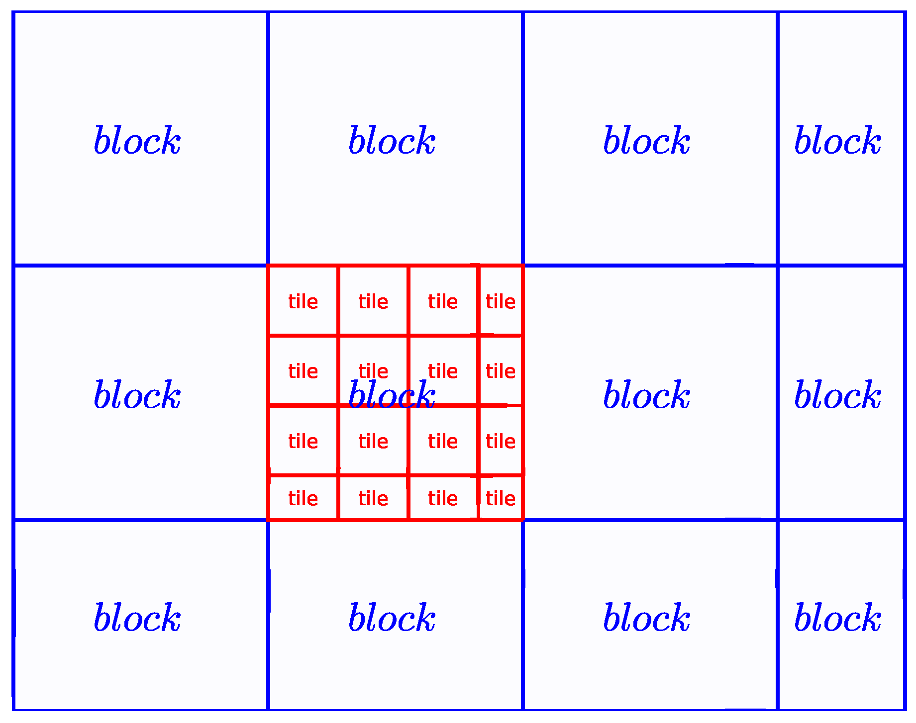
The region of interest (the whole region of the sensed image or the intersection region of the sensed and reference image) is divided into blocks according to the number of target matches.
Each block of the image is divided into small tiles (processing unit) to perform SIFT matching, and in this work, the size of the image tile is .
The corresponding tile is extracted from the reference image (online aerial maps) according to the tile in the sensed image and the initial geometric model.
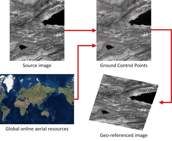
Figure 1.
Flowchart of the proposed matching method.
Figure 1.
Flowchart of the proposed matching method.
Figure 2 illustrates the blocks of an image and the tiles of a block. The aim of image matching is to achieve a reliable control point in each block, and the process will move on to the next block once any tile of the current block succeeds to yield a reliable control point.
Figure 2.
Blocks of an image and tiles of a block.
Figure 2.
Blocks of an image and tiles of a block.
When extracting the corresponding tile from the reference image, the initial geometric model should be utilized, which can be various types: the affine transformation model contained in a georeferenced image or all kinds of imaging models, such as a rigorous sensor model, a polynomial model, a direct linear transformation model, a rational function model (RFM), etc.
Commonly, these imaging models can be defined as a forward model (from the image space to the object space) or an inverse model (from the object space to the image space).
where:
are the coordinates in image space,
are the coordinates in object space,
Z is the elevation,
and are the forward transforming functions of the X and Y coordinates, respectively,
and are the inverse transforming functions of x and y coordinates, respectively.
In the forward model, image coordinates
and elevation
Z are needed to determine the ground coordinates
. With the help of DEM data, however, the ground coordinates
can be determined by the image coordinates
after several iterations. Therefore, the forward model can also be denoted by Equation (
3) if DEM data are available.
With the help of the initial geometric model of the sensed image, the reference image tile can be extracted by calculating its approximate extent. Moreover, to make SIFT matching more efficient and robust, the reference image tile is resampled to a similar resolution as the sensed image tile. The detailed techniques of fetching the reference image tile from online aerial maps will be introduced in
Section 3.
2.2. Extracting SIFT Features
As the reference image tile is resampled to a similar resolution as the sensed image tile, the SIFT detector can be performed in only one octave to get the expected results, and the process becomes much more efficient. In the only octave, the scale space of the image tile is defined as a function,
, that is produced from the convolution of a variable-scale Gaussian,
, with the input image tile,
[
18]:
where
and * is the convolution operation.
Then,
, the convolution of the difference-of-Gaussian (DoG) function and the image tile, which can also be computed from the difference of two nearby scales separated by a constant multiplicative factor
k, is used to detect stable keypoint locations in the scale space by searching the scale space extrema.
Once a keypoint candidate has been found, its location
, scale
σ, contrast
c and edge response
r can be computed [
18], and the unstable keypoint candidates whose contrast
c is less than threshold
(e.g.,
) or whose edge response
r is greater than threshold
(e.g.,
) will be eliminated. Then, image gradient magnitudes and orientations are sampled around the keypoint location to compute the dominant direction
θ of local gradients and the 128-dimensional SIFT descriptor of the keypoint.
2.3. Matching SIFT Features
In standard SIFT, the minimum Euclidean distance between the SIFT descriptors is used to match the corresponding keypoints, and the ratio of closest to second-closest neighbors of a reliable keypoint should be greater than an empirical threshold
, e.g.,
[
18]. However, [
29,
32] pointed out that the
constraint was not suitable for RS images and would lead to numerous correctly-matched eliminations.
In this work, both the
constraint and a cross matching [
32] strategy are applied to find the initial matches. Denoting by
P and
Q the keypoint sets in the sensed and reference image tiles, once either of the following two conditions is satisfied, the corresponding keypoints
and
will be included in the match candidates.
constraint: The ratio of closest to second-closest neighbors of the keypoint
is greater than
, and the keypoint
is the closest neighbor of
. Here, we chose a smaller
rather than 0.8, which is recommended by [
18], to reduce the chance of including too many false matches for RS images.
- Cross
matching: The keypoint is the closest neighbor of in P, and the keypoint is also the closest neighbor of in Q.
Of course, the match candidates usually include a number of false matches, which will be eliminated in the following step.
2.4. Eliminating False Matches
Commonly, some well-known robust fitting methods, such as RANSAC or least median of squares (LMS), are applied to estimate an affine transformation, as well as the inliers from the match candidates. However, these methods perform poorly when the percent of inliers falls much below 50%. In this work, the false matches are eliminated by four steps,
i.e., rejecting by scale ratio, rejecting by rotation angle, rejecting by the coarse similarity transformation (Equation (
6)) using RANSAC and rejecting outliers by the precise affine transformation (Equation (
7)) one by one.
where:
s and θ are the scale parameter and rotation angle parameter of similarity transformation,
and are the translation parameters of similarity transformation in the x direction and the y direction,
are the parameters of affine transformation.
There are a number of reasons for choosing similarity transformation to perform RANSAC estimation instead of affine transformation. Firstly, it is possible for a similarity transformation to model the geometric deformation coarsely in a small tile of an RS image. Secondly, the similarity transformation solution requires less point matches than the affine transformation solution and is also more robust. In addition, the similarity transformation can make full use of the geometric information, such as the scale and dominant direction, of the SIFT keypoints.
(1) Rejecting by scale ratio:
The scale has been computed for each keypoint in the phase of extracting SIFT features (
Section 2.2) and the scale ratio of a pair of corresponding keypoints in the sensed image tile and reference image tile indicates the scale factor between the two image tiles. By computing a histogram of the scale ratios of all match candidates, the peak of the histogram will locate around the true scale factor between the two image tiles [
36]. The match candidates whose scale ratio is far from the peak of the histogram are not likely to be correct matches and, therefore, are rejected from the match candidates. Denoting the peak scale ratio by
, the acceptable matches should satisfy the following criterion:
where
is the scale ratio of a match candidate,
is the scale ratio threshold and
is used in this work. The selection of
will be discussed later at the end of
Section 2.4.
Note that the reference image tile is resampled to a similar resolution as the sensed image tile; the computation of the scale ratio histogram is not necessary. The is expected to be around , even if we do not check the scale ratio histogram.
(2) Rejecting by rotation angle:
Similarly, as the difference of the dominant direction of corresponding keypoints indicates the rotation angle between the two image tiles, a rotation angle histogram can be computed using the dominant directions of the SIFT keypoints in all match candidates. The rotation angle histogram has 36 bins covering the 360 degree range of angles, and the match candidates whose difference of dominant direction is far from the peak of the histogram are rejected. Denoting the peak rotation angle by
, the acceptable matches should satisfy the following criterion:
where
is the dominant directions of the SIFT features in a match candidate,
is the rotation angle threshold and
=15
is used in this work. The selection of
will be discussed later at the end of
Section 2.4.
(3) Rejecting by similarity transformation:
After the first two steps, most of the false matches will be rejected, and the RANSAC algorithm is quite robust to estimate a coarse similarity transformation from the remaining match candidates. Meanwhile, outliers for similarity transformation are also excluded.
(4) Rejecting by affine transformation:
In order to achieve accurate matching results, the remaining match candidates should be further checked by an affine model. Specifically, all of the remaining match candidates are used to find the least-squares solution of an affine transformation, and inaccurate matches, which do not agree with the estimated affine transformation, should be removed. The process will iterate until none of the remaining matches deviates from the estimated affine transformation by more than one pixel.
Note that once fewer than four match candidates remain before or after any of the four steps, the match will be terminated for this tile immediately.
Next, we will provide a discussion on the recommended values of and , and this is based on a matching task using a collection of 1000 pairs of real image tiles that were extracted from different sources of RS images, including Landsat-8, ZY-3, GF-1, etc.
The matching task includes two groups of tests: (1) set
=15
, and let
vary from zero to one; (2) set
, and let
vary from 0
to 360
. A pair of image tiles is called a “matched pair” if the matching process of this image pair yields at least four matches after all four filtering steps. However, for a matched pair, it is possible that not all of the false matches were excluded after the filtering steps, and the results will be untrustworthy. Therefore, only the correctly-matched pairs, whose output matches are all correct, are reliable, and we refer to the percentage of correctly-matched pairs out of all of the matched pairs as the “correct match rate”. In each group of tests, the numbers of matched pairs and correct match rates were obtained for different values of
or
.
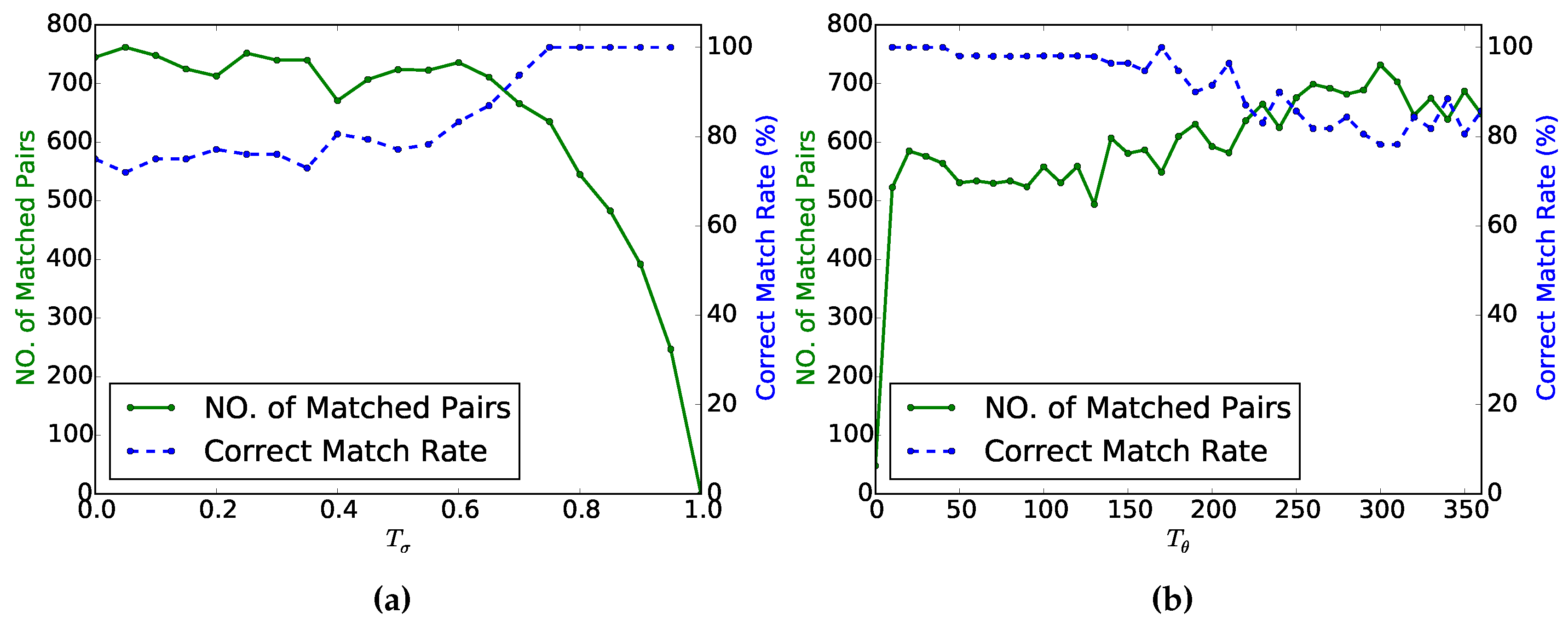
Figure 3a shows the matching results with respect to different values of
, while
Figure 3b shows the matching results with respect to different values of
. According to
Figure 3a, as
increases from zero to one, the number of matched pairs declines, but the correct match rate ascends. According to
Figure 3b, as
increases from 0
to 360
, the number of matched pairs ascends, while the correct match rate declines. To ensure a high correct match rate and enough matches, the value of
should be between 0.70 and 0.85, and the value of
should be between 15
and 30
.
Figure 3.
The numbers of matched pairs and correct match rates for different values of and . (a) The results with respect to different values of ; (b) the results with respect to different values of .
Figure 3.
The numbers of matched pairs and correct match rates for different values of and . (a) The results with respect to different values of ; (b) the results with respect to different values of .
2.5. Refining Position
After the step of eliminating false matches, all of the remaining matches have good agreement (within one pixel) with the local affine transformation. However, the accuracy of the matched points is not high enough considering that they are extracted from the sensed image and reference image independently. Consequently, least squares matching (LSM) is applied to refine the matching results.
It is possible to further include any matches that agree with the final affine transformation from those rejected by error in the phase of eliminating false matches, and then, the new set of matches will be more complete. However, only a pair of matched points is needed for a sensed image tile in the proposed method, even if a large number of matches are found. Therefore, the step of adding missed matches is not included in this work for the sake of efficiency.
Considering that the features having high contrast are stable to image deformation [
32], the keypoint with the highest contrast is chosen from the output of the phase of eliminating false matches. Actually, the high contrast not only guarantees the stability of the keypoints, but also benefits the accuracy of LSM.
LSM is performed in a small region around the SIFT keypoint in sensed image tile, e.g., a template of
, and it is quite efficient. In order to cope with both the geometric deformation and radiometric difference, a geometric model and a radiometric model between two image fragments are modeled together [
16], and the condition equation of a single point is:
where
and
,
are six parameters of geometric transformation,
and
are two radiometric parameters for contrast and brightness (or equivalently gain and offset),
and
are the gray values of a pixel in a source and reference image tile.
The geometric model and the radiometric model are estimated by least squares, and then, we can accurately locate the corresponding point in the reference image tile.
As Equation (
8) is nonlinear, good initial values are required to find the optimal models. Fortunately, the previously-calculated affine transformation provides very good initial values for the geometric parameters, and those of the radiometric parameters can be set as
and
[
16]. Finally, the Levenberg–Marquardt algorithm [
39] is applied to solve the problem.
Below is an example to show the effect of position refinement.
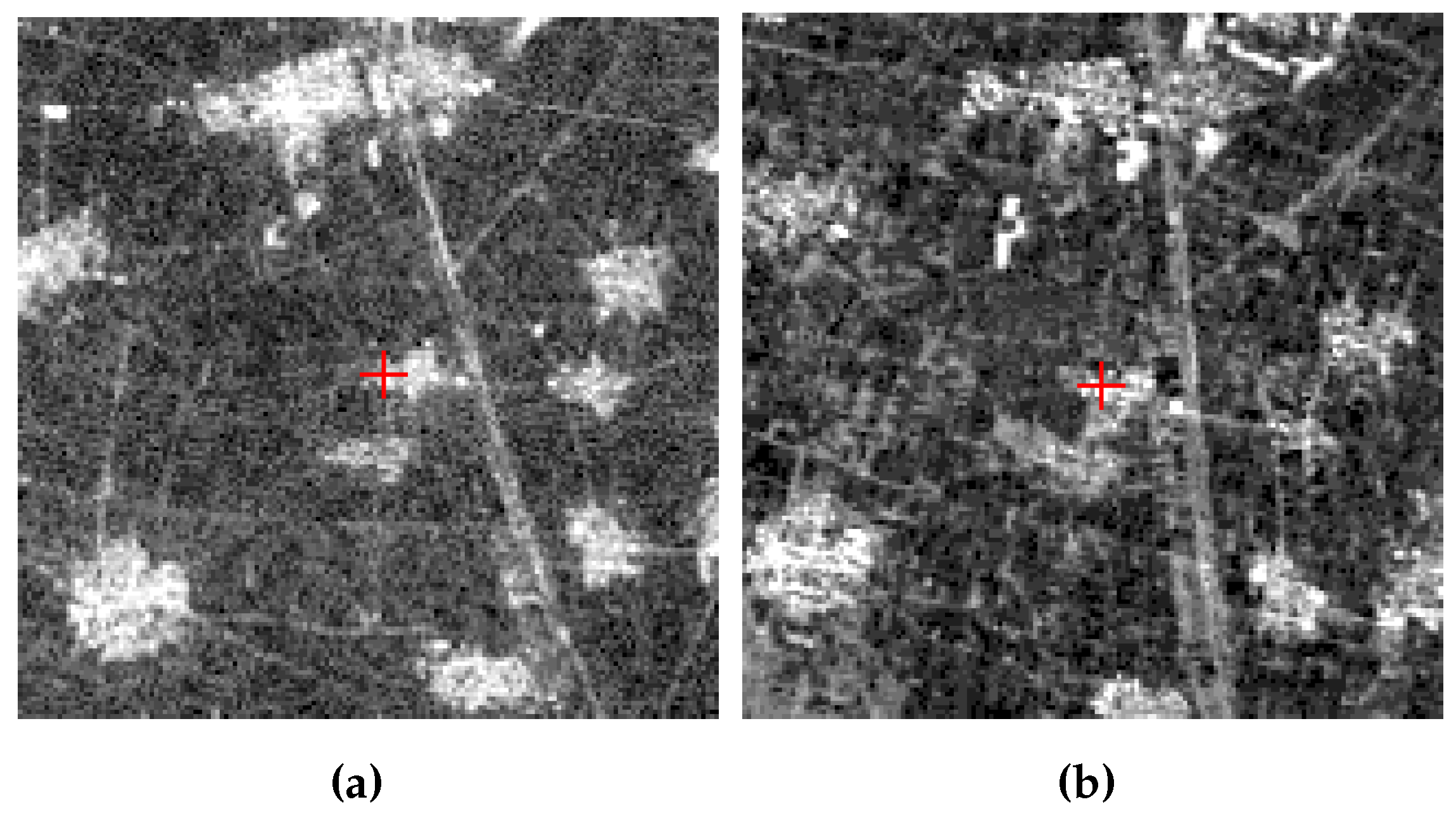
Figure 4 illustrates matched keypoints in the sensed image tile and the reference image tile, and
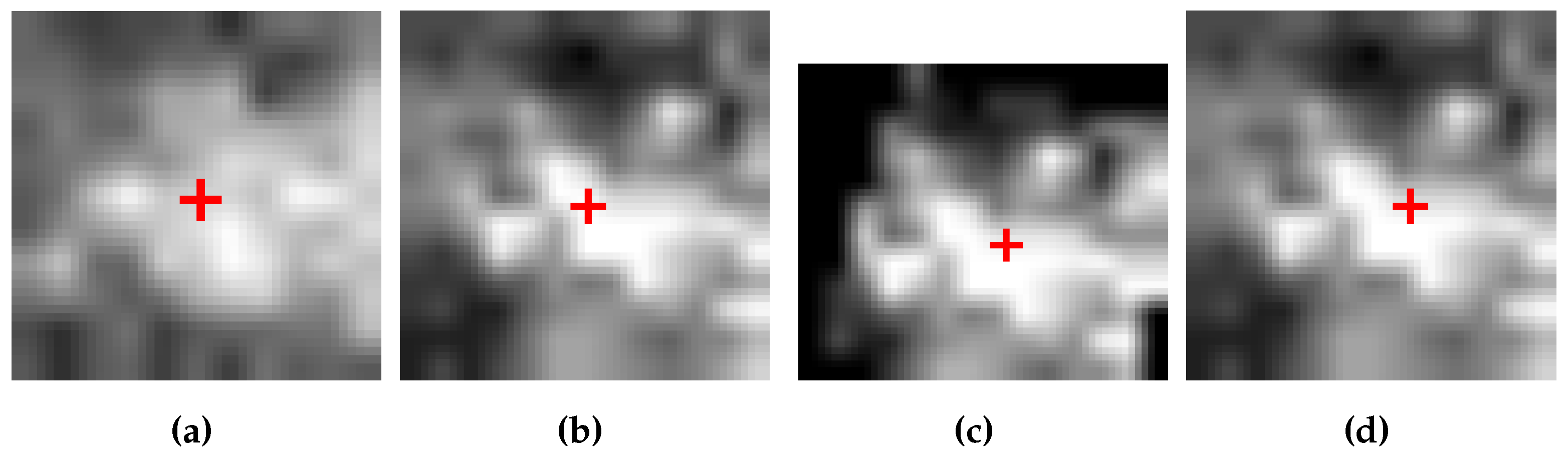
Figure 5 shows the image fragments around the keypoints, as well as the the matched points before and after the phase of position refinement.
Figure 5a,b is the original matching result of SIFT, and it is very difficult to tell whether the matched points in the sensed image and the reference image are corresponding points exactly. However, by applying least squares matching, the warped image fragment in
Figure 5c is in good agreement with the search image fragment in
Figure 5b, both in geometry and radiometry. Consequently, it is very clear that the marked point in
Figure 5c (transformed from the keypoint in
Figure 5a) and that in
Figure 5d (refined by LSM) are corresponding. Meanwhile, one can see that the original SIFT keypoint in
Figure 5b is not accurate enough when comparing to the point in
Figure 5d. Note that the images in
Figure 5 are enlarged by eight times using the cubic interpolation method, and the actual deviation between
Figure 5b,d is about one pixel.
Figure 4.
The matched keypoints in a sensed image tile and a reference image tile. (a) The sensed image tile; and (b) the reference image tile.
Figure 4.
The matched keypoints in a sensed image tile and a reference image tile. (a) The sensed image tile; and (b) the reference image tile.
Figure 5.
(
a) The template image around the SIFT keypoint (marked with a cross) in the sensed image tile; (
b) the search image around the SIFT keypoint (marked with a cross) in the reference image tile; (
c) an image fragment warped from the template image using the geometric model and the radiometric model in Equation (
8), and the cross denotes the SIFT keypoint in the sensed image tile after geometric transformation; (
d) the search image, and the cross denotes the refined keypoint in the reference image tile.
2.6. Summary
According to the number of required control points, the sensed image will be divided into a number of blocks evenly, and only one control point is needed for each block. Then, each block is divided into a number of tiles according to the previously-defined tile size, and once any of the tiles succeeds to produce a control point, the process will move on to the next block. We do not intend to exhaust all of the possible matches, but find a moderate number of control points that are very reliable. Obviously, this method is greedy and therefore efficient.
After the matching of all image blocks is finished, it is easy to further identify potential outliers by checking for agreement between each matched point and a global geometric model, e.g., rigorous sensor model, rational function model, etc. However, hardly any false matches were found in the final matches according to the results of all our tests.
We call the process of matching a pair of a sensed image tile and a reference image tile a “tile trial” (as shown in
Figure 1), and the actual efficiency of the method is decided by the number of tile trial times. If the success rate of tile trial is
(the best case), only one tile trial is performed for each control point, and the number of tile trial times is not related to the size of the sensed image; if the success rate of tile trial is
(the worst case), all of the tiles of the sensed image will be tested, and the number of tile trial times is decided by the size of the sensed image. The success rate of tile trial is related to the similarity between the sensed image and the reference image and the distinction, which can be affected by a number of factors, e.g., the quality (cloud coverage, contrast, exposure,
etc.) of the images, the scale difference, the spectral difference, changes caused by different imaging times,
etc. Additionally, as the tile trial is based on SIFT matching, the success rate is limited if the test images cover a region of low texture, such as water, desert and forest.
Furthermore, the high independence among the image blocks enables a parallel implementation, which can further accelerate the proposed method. The processing of image blocks can be assigned to multiple processors and nodes (computers) in a cluster and, therefore, run concurrently. Parallelization makes full use of the computing resources and exponentially shortens the consumed time of image matching. In this work, we implemented a parallel version on multiple processors, but not on multiple computers.
In addition, the SIFT implementation designed on a graphic process unit (GPU) [
27] may considerably accelerate the process of the tile trial, but it is not yet included in this work.
3. Fetch Reference Image from Online Aerial Maps
In
Section 2.1, we mentioned that the reference image tile can be extracted by calculating its approximate extent, and this section will introduce the detailed techniques to fetch reference image tiles from online aerial maps,
i.e., Google satellite images, Bing aerial images, MapQuest satellite maps and Mapbox satellite images.
3.1. Static Maps API Service
In this work, we use the Static Maps API Service of online aerial maps, i.e., sending a URL (Uniform Resource Locator) request, to fetch the required reference image tiles automatically. For example, the formats of URL request of Google satellite images, Bing aerial images, MapQuest satellite maps and Mapbox satellite images are listed below.
In these URLs, the parameters inside “{}” should be specified, i.e., the longitude and latitude of the center point, zoom level, width and height of the image tile and the API keys. One can apply either free or enterprise API keys from corresponding websites, freely or with a low cost, and the calculation of the other parameters will be introduced in the following sections.
3.2. Zoom Level
For online global maps, a single projection, Mercator projection, is typically used for the entire world, to make the map seamless [
40]. Moreover, the aerial maps are organized in discrete zoom levels, from 1 to 23, to be rendered for different map scales. At the lowest zoom level,
i.e., 1, the map is
pixels, and once the zoom level is increased by one, the width and height of the map expand twice.
Consequently, in order to fetch the corresponding reference image tile, we need to firstly determine the zoom level, which is related to the ground sample distances (GSD) of the sensed image tile. Similar to the relative scale between the sensed image and the reference image, the GSDs of the sensed image are not necessarily constant in a whole image, and the local GSDs of an image tile can be calculated by the formula:
where:
and are the ground sample distances in x direction and y direction,
and are the image coordinates of the center point of the sensed image tile,
and
are the forward transforming functions of the
X and
Y coordinates, which are described in Equation (
3).
On the other hand, the GSDs (in meters) of online aerial maps vary depending on the zoom level and the latitude at which they are measured, and the conversion between the GSD and nearest zoom level is described by Equation (
10),
where:
is the earth radius, for which 6,378,137 meters is used,
ϕ is the latitude at which it is measured,
is the ground sample distance (in meters), both in the x direction and y direction,
n is the zoom level,
is an operator to find the nearest integer.
Equation (
10) can be applied to find the nearest zoom level according to the GSD of the sensed image tile (the mean value of those in the
x direction and the
y direction) calculated by Equation (
9).
3.3. Width and Height
By providing the rectangle extent of the sensed image tile, the corresponding geographic coordinates (longitude and latitude) of the four corners can be calculated by the initial forward transforming functions in Equation (
3). In order to find the extent of the required reference image tile, the geographic coordinates,
λ and
ϕ, should be converted to the image coordinates,
x and
y, in the map of the nearest zoom level,
n, according to Equation (
11) [
40],
where
λ and
ϕ are the longitude and latitude.
Then, the extent of reference image tile is the minimum boundary rectangle of the four corners in the map of zoom level n, and the width and height of the tile are known, accordingly.
3.4. Center Point
Next, we need to calculate the geographic coordinates of the center point of reference image tile, and the following inverse transformation from image coordinates,
x and
y, in the map of the nearest zoom level,
n, to geographic coordinates,
λ and
ϕ, will be used,
Equation (
12) is derived from Equation (
11) directly, and it will be used again when the matched points in the sensed and reference image tile are found, as the image coordinates in the reference image tile should be converted to geographic coordinates to obtain ground control points.
3.5. Resizing
Given the nearest zoom level, the width and height of the image tile, the longitude and latitude of the center point and the API keys, the Static Maps API service can be used to download the required reference image tile from the online aerial images. However, the GSD of the downloaded reference image tile may not be very close to that of the sensed image tile, since the zoom level is discrete. The downloaded image tile needs to be further resampled to a similar resolution as the sensed image tile for the sake of efficiency and robustness, according to the relative scale between the two image tiles, which can be calculated by dividing the GSD of the sensed image tile by that of the online reference image tile.
3.6. Summary
The scene of a RapidEye image captured in 2010 is used to show an example of online matching. The image is of Oahu, Hawaii, and the spatial resolution is 5 m.
Figure 6 shows a tile of the RapidEye image matched with different online aerial maps, including Google satellite images, Bing aerial images, MapQuest satellite maps and Mapbox satellite images. Note that we intentionally chose a scene in the USA, as the MapQuest satellite maps of high zoom levels (higher than 12) are provided only in the United States.
From
Figure 6, one can see that in the same range, the data sources of the four kinds of online aerial maps are not the same. In practically applications, different online aerial maps can be used for complementation.
Figure 6.
Example of online matching, and the matched points are marked by cross. (a) to (d) are matching results using Google satellite images, Bing aerial maps, MapQuest satellite maps and Mapbox satellite images, respectively. In each figure, the left is the RapidEye image tile, while the right is the online aerial map.
4. Experiments and Analysis
In this section, several groups of experiments are carried out to check the validity of the proposed method, and all experiments are performed on a 3.07-GHz CPU with four cores.
4.1. Robustness
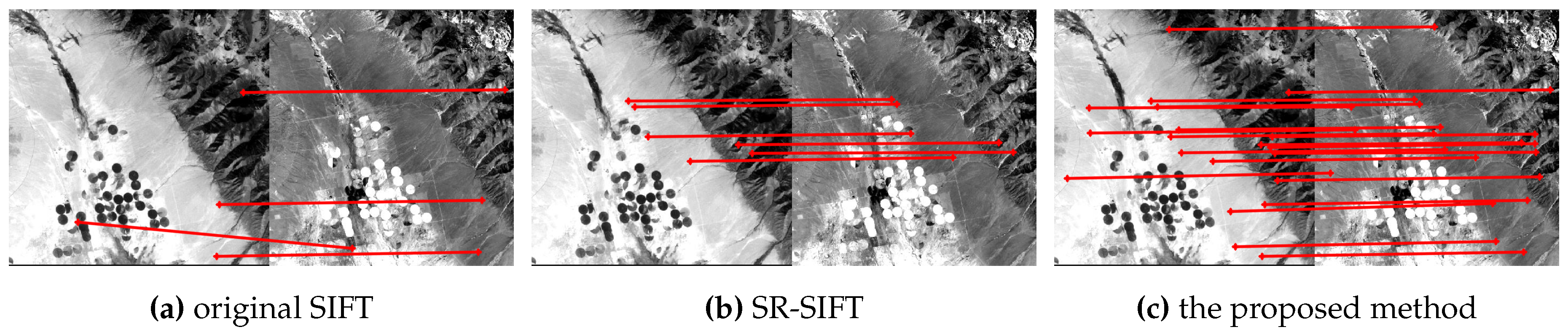
To show the superiority of the matching strategy of the proposed method, we carry out comparative tests with three methods: the proposed method, the ordinary SIFT [
18] and SR-SIFT [
34], which is claimed to be more robust than ordinary SIFT. In the ordinary SIFT matching method, match candidates are found by using the distance ratio constraint of closest to second-closest neighbors, and outliers are eliminated by using the RANSAC algorithm and affine transformation. In the SR-SIFT method, scale restriction is applied to exclude unreasonable matches before the RANSAC filtering. The distance ratio threshold
is applied in all of the methods.
Figure 7 shows the results of the three methods when applied to a pair of AVIRIS image tiles (visible and infrared).
Figure 7.
Matching results of the AVIRIS visible image tile (left) and the AVIRIS infrared image tile (right), using three different methods. (a) The result of original SIFT (four matches are found, including a wrong match); (b) the result of SR-SIFT (six correct matches are found); and (c) the result of the proposed method (20 correct matches are found).
From
Figure 7, we can see that the original SIFT yields the poorest matching results, while SR-SIFT provides more correct matches. However, the best results come from the proposed method, not only the quantity of correct matches, but also the distribution of matched points.
We also test more than 100 successfully-matched tiles, from six pairs of RS images, including Landsat-5
vs. Landsat-5 (captured at different times), Huanjing-1 (HJ-1)
vs. Landsat-8, Gaofen-1 (GF-1)
vs. Bing aerial maps, Ziyuan-3 (ZY-3)
vs. RapidEye, GF-1 Multispectral (MSS)
vs. GF-1 Panchromatic (PAN) (captured simultaneously), Kompsat-2
vs. Worldview-1, and the numbers of remaining matches after each step of the methods are noted.
Table 2 shows the results of 12 pairs of tiles (two pairs of tiles are randomly selected from each dataset).
Table 2.
The number of remaining matches after each step in the three methods.
Table 2.
The number of remaining matches after each step in the three methods.
| Datasets | Tiles | Proposed Method | | Ordinary SIFT | | Ordinary SIFT |
|---|
| S1 | S2 | S3 | S4 | S5 | S6 | | S1 | S2 | | S1 | S2 | S3 |
|---|
| D1 | Tile 1 | 125 | 88 | 33 | 23 | 17 | 17 | | 19 | 14(11) | | 19 | 17 | 14(11) |
| Tile 2 | 98 | 60 | 17 | 8 | 5 | 5 | | 10 | 6(4) | | 10 | 9 | 7(6) |
| D2 | Tile 1 | 142 | 91 | 20 | 15 | 8 | 9 | | 8 | 8(6) | | 8 | 8 | 8(6) |
| Tile 2 | 124 | 88 | 18 | 15 | 10 | 11 | | 15 | 13(9) | | 15 | 15 | 13(9) |
| D3 | Tile 1 | 122 | 72 | 31 | 14 | 7 | 8 | | 14 | 10(5) | | 14 | 14 | 10(5) |
| Tile 2 | 124 | 91 | 52 | 44 | 26 | 28 | | 55 | 49(26) | | 55 | 52 | 50(25) |
| D4 | Tile 1 | 130 | 87 | 40 | 9 | 6 | 7 | | 25 | 16(5) | | 25 | 23 | 17(6) |
| Tile 2 | 153 | 114 | 69 | 16 | 8 | 9 | | 37 | 34(3) | | 37 | 36 | 34(3) |
| D5 | Tile 1 | 215 | 206 | 113 | 75 | 75 | 105 | | 195 | 104(102) | | 195 | 190 | 103(101) |
| Tile 2 | 216 | 200 | 100 | 69 | 68 | 101 | | 184 | 102(98) | | 184 | 182 | 102(98) |
| D6 | Tile 1 | 129 | 76 | 19 | 7 | 5 | 5 | | 3 | 0(0) | | 3 | 3 | 0(0) |
| Tile 2 | 115 | 73 | 26 | 8 | 6 | 7 | | 10 | 4(2) | | 10 | 9 | 5(3) |
From
Table 2, the following points can be drawn:
The results of ordinary SIFT and SR-SIFT are similar, and a simple scale restriction filter seems not helpful to find correct matches. Specifically, in most cases (except for Dataset 5), the distance ratio constraint excludes a number of correct matches and sometimes results in failure (e.g., in Dataset 6). By applying cross matching, the proposed method includes much more initial match candidates, although many of them are false matches.
The percentage of outliers in the initial match candidates is usually greater than , and the RANSAC algorithm is not robust enough to identify correct subsets of matches; thus, it frequently fails or yields untrustworthy results. On the other hand, in the proposed method, four steps of outlier rejecting can eliminate all of the false matches. Actually, after the first two steps of rejecting (by the scale ratio and by the rotation angle), most of the outliers will be cast out.
Commonly, only a few matches will be added in Step 6 of the proposed method, except for Dataset 5, in which the correct matches are plentiful. Consequently, Step 6 can be omitted, without affecting the final result too much.
The ordinary SIFT matching method performs quite well for Dataset 5, in which the sensed image and reference image were captured simultaneously from the same aircraft and in the same view angle. With little variation in content, illumination and scale, the SIFT descriptor is very robust and distinctive, and the distance ratio constraint identified most of the correct matches. Then RANSAC algorithm manages to find reliable results, since the match candidates contain fewer than outliers.
4.2. Efficiency
In order to show the efficiency of the proposed method, SiftGPU [
27], which is the fastest version of SIFT to our best knowledge, is applied to carry out comparative tests with the proposed method. The implementation of SiftGPU is provided by Wu C. in [
27].
Two scenes of GF-2 PAN images in Beijing, China, which were acquired on 3 September 2015 and 12 September 2015, respectively, are used to perform the matching tests. GF-2 is a newly-launched Chinese resource satellite; the spatial resolution of its panchromatic image is around 0.8 m, and the size of an image scene is around 29,000 × 28,000 pixels.
Figure 8.
Matching results of GF-2 PAN images, using SiftGPU and the proposed method. In each sub-figure, the left is the image captured on 3 September 2015 and the right is the image captured on 12 September 2015. The matched points are labeled by the same numbers, and red crosses stand for correct matches, while yellow crosses stand for wrong matches. (a) The result of SiftGPU (71 correct matches and 11 wrong matches); and (b) the result of proposed method (30 correct matches are found).
SiftGPU spends 19.4 s to find 82 matched points (including 11 incorrectly matched points) from the two scenes of GF-2 images, while the proposed method spends 20.6 s to find 30 matched points, and the matching results are shown in
Figure 8. Although SiftGPU yields more matches within less time, the distribution and the correctness of the results of the proposed method (as shown in
Figure 8b) are obviously superior to those of SiftGPU (as shown in
Figure 8a). SiftGPU makes full use of the computing resource of the computer devices and is quite efficient when processing large images, and 15,030 and 16,291 SIFT keypoints are extracted from the two images respectively within a dozen seconds. However, finding the corresponding keypoints is difficult, as the large scene makes the descriptors of SIFT keypoints less distinctive. Moreover, the serious distortion of the satellite images also makes it difficult to identify the outliers from matched points; the residual errors of the 71 correctly matched points are more than 100 pixels when fitted by a three-degree 2D polynomial function.
Actually, SiftGPU frequently fails to provide sound results for very large satellite images according to our experimental results, despite its outstanding efficiency.
In summary, the proposed method is almost as fast as SiftGPU, but provides more reliable results.
4.3. Accuracy
In
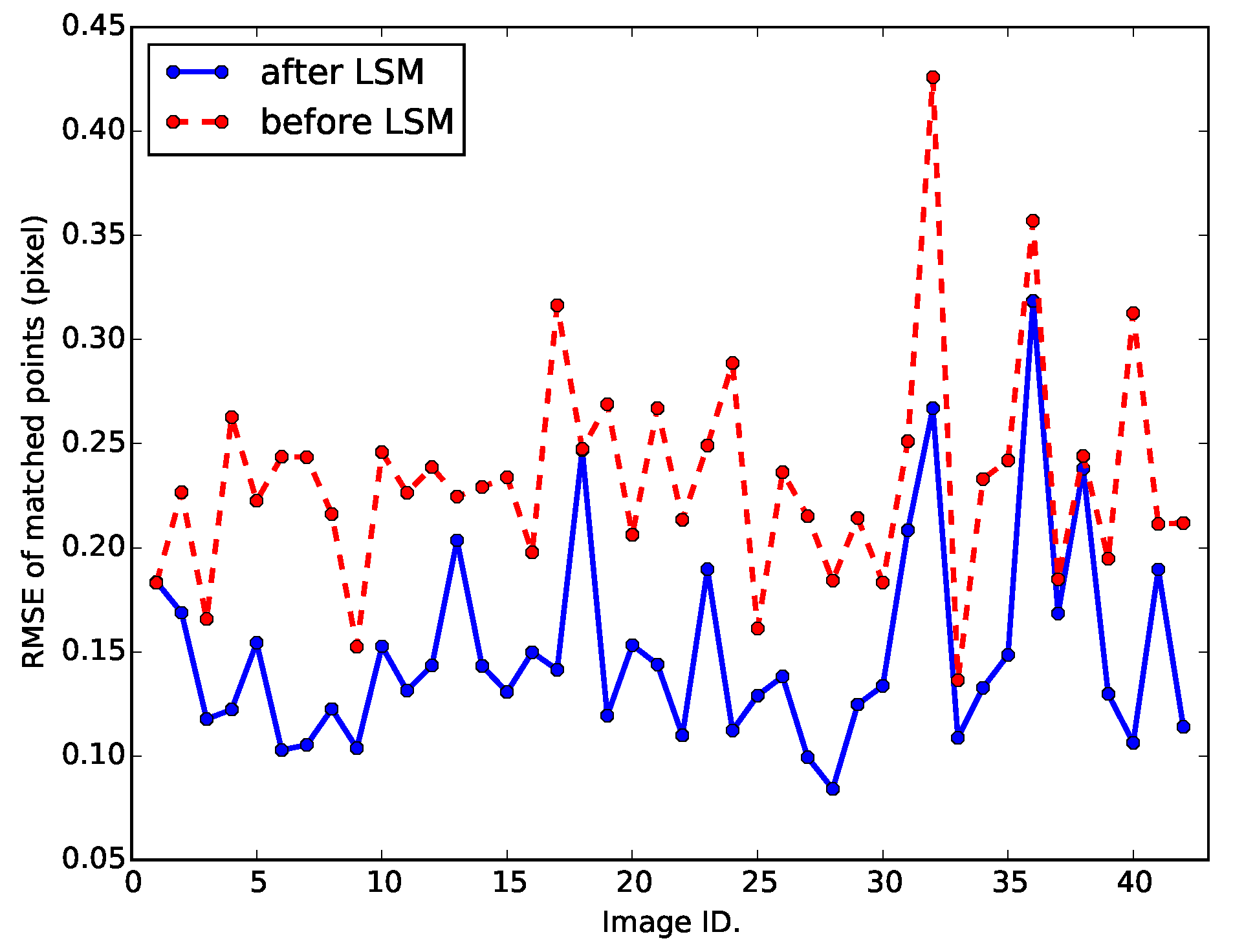
Section 2.5, an example has shown the effect of least squares match (LSM) refinement, and in this section, 42 scenes of the GF-1 MSS image are used to further evaluate the accuracy of the proposed method.
Firstly, the original GF-1 images are rectified based on the vendor-provided RPC model with constant height zero and projected in longitude and latitude. Secondly, 25 check points, , are collected between each pair of the original image and the rectified image using the proposed method. Finally, the geographic coordinates, , of the check point in the rectified images are transformed into the image coordinates, , in the original images using the inverse transformation of the vendor-provided RPC model, and then, the biases between the matched points can be measured by the difference of the image coordinates, . The results before and after LSM refinement are compared to show the accuracy improvement of the proposed method.
Figure 9 shows the root mean square biases of matched points before and after LSM refinement in each image, and one can see that in most of the tests, the accuracy of the matched points is notably improved after LSM refinement.
There are several reasons to use this experimental scheme. Geometric transformation, especially longitude and latitude projection, usually results in distortion of the image and then increases the uncertainty of the position of detected SIFT features, while image distortion commonly exists in practical image matching tasks. In addition, by performing image matching between the original image and the rectified image, the ground truth of the bias should be zero, since the parameters of geometric transformation are already known. Moreover, the least squares match is performed in a small patch and is independent of the global transformation (vendor-provided RPC model); thus, the agreement between the matched points and the global transformation can be applied to evaluate the accuracy of matching, objectively. Note that the position biases between matched points may not be exactly zero, due to the errors introduced by interpolation.
Figure 9.
Root mean square biases of matched points before and after least squares match (LSM) refinement.
Figure 9.
Root mean square biases of matched points before and after least squares match (LSM) refinement.
4.4. Practical Tests
To evaluate the proposed method, four scenes of RS images, including Landsat-5, China-Brazil Earth Resources Satellite 2 (Cbers-2), Cbers-4, ZY-3, GF-2, Spot-5, Thailand Earth Observation System (Theos) and GF-1, are used to perform online matching, while Bing aerial images are utilized as the reference images. For each image, the proposed matching method is used to automatically collect control points, which are then applied to rectify the sensed image, and finally, 20 well-distributed check points are manually collected from the rectified image and reference images (Bing aerial images) to evaluate the matching accuracy.
Table 3 shows the general information of the test images used in these experiments.
Table 3.
General information of the test images.
Table 3.
General information of the test images.
| Test No. | Data Source | Band | Image Size | GSD (m) | Acquisition Time | Elevation | Location | Initial Model |
|---|
| 1 | Landsat-5 | Band 4 | 6850 × 5733 | 30 | 2007 | 566 to 4733 | China-Sichuan | Rigorous |
| 2 | Cbers-2 | Band 3 | 6823 × 6813 | 20 | 2008 | 486 to 1239 | Brazil-Grão Mogol | Affine |
| 3 | Cbers-4 P10 | Band 3 | 6000 × 6000 | 10 | 2015 | 813 to 1514 | South Africa-Buysdorp | Rigorous |
| 4 | ZY-3 | Band 1 | 8819 × 9279 | 5.8 | 2014 | 769 to 2549 | China-Shaanxi | RPC |
| 5 | GF-2 | Band 1 | 7300 × 6908 | 3.2 | 2015 | 273 to 821 | China-Ningxia | RPC |
| 6 | Spot-5 | Pan | 33,730 × 29,756 | 2.5 | 2010 | 17 to 155 | China-Wuhan | Affine |
| 7 | Theos | Pan | 14,083 × 14,115 | 2 | 2014 | 1285 to 1736 | China-Xinjiang | Affine |
| 8 | GF-1 | Pan | 18,192 × 18,000 | 2 | 2014 | 3080 to 4159 | China-Qinghai | RPC |
As shown in
Table 3, different initial image models of the sensed image are utilized, including the rigorous sensor model, affine transformation contained in georeferenced images, the vendor-provided RPC model,
etc. The rigorous sensor model of Landsat-5 is provided by the open source software OSSIM [
41] and the rigorous sensor model of the Cbers-4 image is built according to the 3D ray from the image line-sample to ground coordinates in the WGS-84 system. The RPC models of the ZY-3, GF-2 and GF-1 images are provided by the vendors. The Spot-5, Cbers-2 and Theos images are processed to the L2 level of correction, and the affine transformation models contained in images are used as initial imaging models.
Cbers-2 (Test 2), Cbers-4 P10 (Test 3), Spot-5 (Test 6) and Theos (Test 7) images are rectified based on the terrain-dependent RPC (TD-RPC) model. Landsat-5 image in Test 1 is rectified based on the rigorous sensor model, and RPC refinement is applied to rectify the ZY-3 (Test 4), GF-2 (Test 5) and GF-1 (Test 8) images. Therefore, we intend to find 100 GCPs for each image in Tests 2, 3, 6 and 7, while 30 GCPs are required for each image in Tests 1, 4, 5 and 8. Note that all of the TD-RPC models in the tests are calculated using
-Norm-Regularized Least Squares (L1LS) [
42] estimation method, to cope with the potential correlation between the parameters.
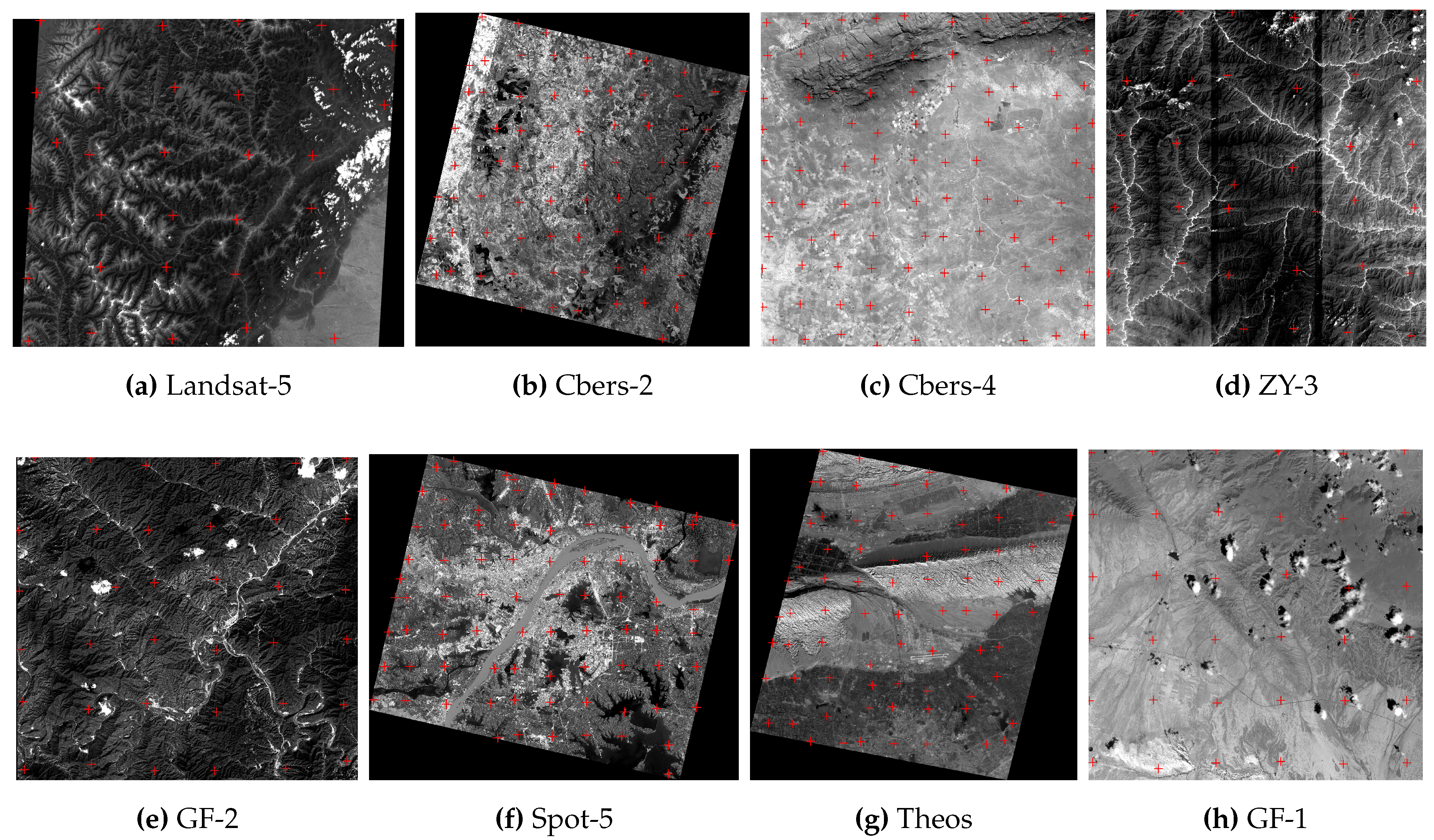
Figure 10 shows the distribution of matched points in Test 1 – Test 8, and
Table 4 shows more results for each test, including the number of correct matches, consumed time, the model used for geometric rectification and the RMSE of check points.
Figure 11 is the comparison between the sensed images and the online Bing aerial maps in Tests 4, 6, 7 and 8 using the “Swipe Layer” tool in ArcGIS Desktop, and ArcBruTile [
43] is used to display the Bing aerial maps in ArcGIS Desktop.
In this section, the spatial resolution of the test image varies from 30 m to 2 m, but the very high resolution (less than 1 m) RS images are not included, as the geometric accuracy of the online aerial maps is limited. In this sense, we can successfully find enough GCPs for very high resolution images from the online aerial maps, but the accuracy of the GCPs is not guaranteed.
According to
Figure 3, and the test results in
Figure 10,
Figure 11 and
Table 4, one can see that:
Various kinds of geometric models can be used as the initial imaging model, including rigorous models for different sensors, the vendor-provided RPC model and the affine transformation model contained in georeferenced images.
The proposed method is successfully applied to match images captured in different imaging conditions, e.g., by different sensors, at different times, at different ground sample distances, etc.
Sufficient and well-distributed GCPs are efficiently collected for sensed images of different spatial resolutions, and the biases between the sensed images and online aerial maps are corrected after the process of image matching and geometric rectification.
It is a very convenient and efficient way to automatically collect GCPs for the task of geometric rectification of RS images, as there is no need to manually prepare reference images according to the location and spatial resolution of sensed images.
Note that the process of matching online is commonly a bit more time consuming than matching locally, since sending requests and downloading image tiles from online aerial maps may take more time than extracting image tiles from local reference images.
Figure 10.
Distribution of matched points (marked by a cross) and sensed images in online image matching tests. (a–h) are the results of Landsat-5, Cbers-2, Cbers-4, ZY-3, GF-2, Spot-5, Theos and GF-1 images, respectively.
Figure 10.
Distribution of matched points (marked by a cross) and sensed images in online image matching tests. (a–h) are the results of Landsat-5, Cbers-2, Cbers-4, ZY-3, GF-2, Spot-5, Theos and GF-1 images, respectively.
Table 4.
Test results of online image matching.
Table 4.
Test results of online image matching.
| Test No. | Required GCPs | Block No. | Correct Matches | Run-Time (S) | Rectification Model | RMSE (Pixel) |
|---|
| 1 | 30 | 6 × 6 | 32 | 7.11 | Rigorous | 1.24 |
| 2 | 100 | 10 × 10 | 75 | 41.00 | TD-RPC | 1.01 |
| 3 | 100 | 10 × 10 | 97 | 42.94 | TD-RPC | 0.84 |
| 4 | 30 | 6 × 6 | 35 | 23.48 | RPC-Refine | 1.82 |
| 5 | 30 | 6 × 6 | 36 | 16.01 | RPC-Refine | 1.35 |
| 6 | 100 | 10 × 10 | 82 | 45.93 | TD-RPC | 1.53 |
| 7 | 100 | 10 × 10 | 77 | 67.41 | TD-RPC | 1.46 |
| 8 | 30 | 6 × 6 | 36 | 21.96 | RPC-Refine | 1.77 |
Figure 11.
Layer swiping between sensed images and online aerial maps in Tests 4, 6, 7 and 8. (a) and (b) are from Test 4, and the top ones are Bing aerial maps, while the lower one in (a) is the warped ZY-3 image using vendor-provided RPC and the lower one in (b) is the rectified ZY-3 image using RPC refinement; (c) and (d) are from Test 6, and the left are Bing aerial maps, while the right one in (c) is the Spot-5 image of Level 2 and the right one in (d) is the rectified Spot-5 image using terrain-dependent RPC; (e) and (f) are from Test 7, and the right are Bing aerial maps, while the left one in (e) is the Theos image of Level 2 and the left one in (f) is the rectified Theos image using terrain-dependent RPC; (g) and (h) are from Test 8, and the upper are Bing aerial maps, while the lower one in (e) is the warped GF-1 image using vendor-provided RPC and the lower one in (f) is the rectified GF-1 image using RPC refinement.


