Change Detection of Submerged Seagrass Biomass in Shallow Coastal Water

Abstract

Satellite remote sensing is an advanced tool used to characterize seagrass biomass and monitor changes in clear to less-turbid waters by analyzing multi-temporal satellite images. Seagrass information was extracted from the multi-temporal satellite datasets following a two-step procedure: (i) retrieval of substrate-leaving radiances; and (ii) estimation of seagrass total aboveground biomass (STAGB). Firstly, the substrate leaving radiances is determined by compensating the water column correction of the pre-processed data because of the inherent errors associated with the geometric and radiometric fidelities including atmospheric perturbations. Secondly, the seagrass leaving radiances were correlated to the corresponding in situ STAGB to predict seagrass biomass. The relationship between STAGB and cover percentage was then established for seagrass meadows occurring in Merambong, Straits of Johor, Malaysia. By applying the above-mentioned approach on Landsat Thematic Mapper (TM) acquired in 2009 and Operational Land Imager (OLI) data acquired in 2013, the resulting maps indicated that submerged STAGB in less clear water can be successfully quantified empirically from Landsat data, and can be utilized in STAGB change detection over time. Data validation showed a good agreement between in situ STAGB and Landsat TM (R² = 0.977, p < 0.001) and OLI (R² = 0.975, p < 0.001) derived water leaving radiances for the studied seagrass meadows. The STAGB was estimated as 803 ± 0.47 kg in 2009, while it was 752.3 ± 0.34 kg in 2013, suggesting a decrease of 50.7 kg within the four-year interval. This could be mainly due to land reclamation in the intertidal mudflat areas performed, with a view to increase port facilities and coastal landscape development. Statistics on dugong sightings also supports changes in STAGB.

1. Introduction

Quantifying seagrass total aboveground biomass (STAGB) is vital for various inputs of coastal related studies and ecology. Seagrass biomass in coastal ecosystem has been reported at a regional [1,2,3] and local scale [4,5,6]. It is considered an important indicator of coastal ecosystem health, used for sustainable coastal development [7], and is used to estimate total carbon as it sequesters. As some marine species such as dugong and sea turtle use seagrasses as their primary food source, degradation of seagrass biomass will create their food scarcity and consequently may reduce their abundance and make those threatened species more vulnerable [8]. Seagrass biomass is a barometer for assessing impacts of coastal landscape alteration on seagrass dynamics, species composition and water clarity [9]. Being seagrass is a component of coastal ecosystem and has the ability to reflect global climate change, biomass quantification has gathered more attention in recent studies at global, regional and local levels. Local level seagrass biomass and associated biophysical (marine environment) changes are used for assessing changes in seagrass abundance and associated species, and understanding climate change impacts at regional and global levels. Thus, this seagrass parameter is used as a proxy for understanding coastal health and developing coastal management plans.

Seagrass naturally has the ability to adapt in a range of water clarities—from mostly clear waters to rarely less clear waters. The survival, growth and abundance of seagrasses are influenced by the biophysical factors including underwater light, transparency, nutrients and temperature [10]. Malaysia has a total of 4809 km coastline, of which 492 km is of Johor [11] that includes 25.2 km Merambong coastline. Coastal areas of Merambong have experienced rapid coastal development. Although coastal development brings about prosperous economies, activities related to this makes the seawater less clear and optimal seagrass biomass growth is retarded. The changes in water clarity and other environmental settings may cause simultaneous changes in STAGB over the years. The seagrass extent, coverage and shoot density are important factors that influence the significant changes in the seagrass biomass [12,13] due to variations of local climate, temperature, population density along the coastal and urban areas. These changes can be efficiently documented using remote sensing methods. In the coastal and ecological management perspectives, quantification of submerged STAGB changes using remote sensing is essential and timely.

Seagrass meadows occurring in coastal waters can be found in two different habitats. The first is seagrass meadows that remain inundated during low tide known as intertidal and the other is, seagrass meadows that remain submerged even during the lowest low tide known as subtidal [14]. In the tropical coastal waters, seagrasses are commonly occurring in shallow water (≤5 m). In Malaysia, the tide height remains lowest for 2–3 h during mid-year to July, particularly in the southern part of Johor. During this period, intertidal seagrass meadows become exposed to the sun, which allows seagrass data collection through direct sampling. Quantification of seagrass biomass, either using field survey or remote sensing methods, can efficiently be perfomed at that golden time. There is less possibility of coincidence between the subtidal seagrass meadows to be fully exposed and the satellite overpass time. Hence, monitoring the subtidal and intertidal seagrass meadows of Malaysia often experiences difficulties particularly when the satellite image acquisition and tide heights do not synchronize throughout the year. This issue makes STAGB data acquisition and quantification more challenging. Low water clarity, in other words, high concentration of floating particles, complicates STAGB estimation from the satellite images.

For monitoring the STAGB changes, if the traditional field-based methods are followed, it will require multi-temporal visits to seagrass meadows to manually record the seagrass coverage and those types of survey techniques are expensive, time-consuming and also cause physical damage to seagrasses during sample collection. STAGB change analysis using a remote sensing method can be an alternative and effective method because of its cost-effectivenes, and consistent, repetitive and synoptic coverage. Studies on STAGB changes using remote sensing methods are limited, as evidenced by fewer publications. The limiting factors include: (a) inherent spatial and spectral characteristics of multi-spectral sensors; (b) fluctuations of temperature in tropical countries; (c) satellite over pass time; (d) sampling from remote locations; (e) changes in seagrass biomass over the year. Remote sensing methods suitable for estimating submerged STAGB under less clear water is rarely reported and explored. The high annual precipitation in the tropical areas causes water clarity lower than that of northern and southern latitudes. Similar studies had been conducted in clear coastal waters and documented in [15,16], that were mostly in clear waters (Case-1) of Australia. Less efforts are required to obtain good STAGB results from the analysis of the images acquired during low spring tides, and as when seagrass leaves are exposed. Quantification of STAGB for the seagrasses occurring in Case-2 water coupled with high concentration of yellow matter, may make the task difficult because of light attenuation in water column. In this paper, a remote sensing approach for STAGB quantification is implemented for less clear water, which is an extension of earlier research [17,18]. The satellite image band differencing method is used in detecting STAGB changes. To date, few studies have documented STAGB changes in submerged seagrasses, occurring especially in less clear waters.

While STAGB quantification in less clear water is challenging, the water column effect is vital to handle the challenges mentioned above. Prior to this, the robustness of water column correction technique called bottom reflectance index (BRI) by [19] to detect the changes in submerged STAGB is tested on the multi-species seagrass meadow environment. In addition, we applied the empirical method on Landsat images with 30 m spatial resolution that have a large spatial coverage and are free to download. Through this study, we intend to highlight the great potential of multi-temporal Landsat data and remote sensing method for (a) identification and mapping of seagrass extent; (b) quantification of submerged STAGB in Case-2 coastal water; (c) STAGB change detection and its assessment. A number of key research questions emerged, including how the dynamic changes of STAGB can be quantified using spatio-temporal remote sensing data. Hence, this paper emphasized the changes of STAGB in mixed-species composition, seagrass extent and empirical use BRI on Landsat Thematic Mapper (TM) and Operational Land Imager (OLI) images to quantify submerged STAGB in partially turbid coastal shallow Case-2 waters [20] at the southern tip of the Malaysian Peninsula. Several assumptions are considered including: (a) the tropical coastal region has highly stable climatic condition and air temperature; (b) insignificant changes occur during monsoon season; (c) less dynamic changes of seagrass coverage occur over the years; (d) less seasonal variation throughout the year; and (e) the utilization of similar spatial and spectral specifications of sensor so that variation of satellite image characteristics is minimal. Subsequently, using the sufficient number of sampling of seagrass at two year intervals at similar locations, within similar sampling quadrat size, the changes of seagrass extent, distribution and its STAGB can be performed using remote sensing approach and regional algorithm of water column correction. Thus, STAGB quantification of submerged shallow seagrass empirically developed after implementation of water column correction in case-2 water.

2. Materials and Methods

2.1. Study A—Merambong Shoal

Seagrass aboveground biomass data was collected from the seagrass meadows occurring in Merambong shoal, located in the Sungai Pulai estuary, Straits of Johor, Malaysia (Figure 1). This study site is in the northeastern side of the Merambong Island, one of the most significant natural marine frontiers between Malaysia and Singapore. It is 1.8 km in length from north to south and 200 m in width from east to west, covering latitude of 01°19.979′ North and longitude of 103°35.965′ East; total approximate area is 42.6 km² which covers Tanjung Kupang and Tanjung Adang.

It is the largest single tract of seagrass meadow in Malaysia, surrounded by Case-2 water. This area is home to myriad marine biodiversity and extensive development of subtropical benthic habitat features in shallow to deep waters [21]. Out of 60 seagrass species found worldwide, 15 species are found in this region [22,23], and 10 species are found on this shoal. Submerged benthic habitats present on site during fieldwork were (a) seagrass: Enhalus acoroides, Halophila ovalis, Cymodocea serrulata and Halodule uninervis; (b) seaweed: Sargassum, Chaetomorpha minima [12,24], and (c) insignificant population of fringing coral reef [10], with a bottom depth ranging from 0.3 m to 35 m where, typically, the seagrass habitat is bounded to water depth less than 4 m. Many seagrass patches are always submerged and randomly distributed in this area. The shoal is mostly covered by Enhalus acoroides and paddle-shaped Halophila ovalis. Moreover, this area is intensively used for many scientific research activities.

2.2. Materials

Two main material sets were used in this study, namely the satellite remote sensing data and field samples from in situ observations used for ground truthings. The Landsat 5 TM and Landsat 8 OLI data, which have different characteristics, were used to detect STAGB changes (see Figure 2). In addition, hydrographical charts acquired from the National Hydrographic Centre of Malaysia was used to obtain the depth information.

An underwater camera and GPS were used during sea truth data collection (15 February 2009 and 8 June 2013) to record the seagrass patchiness, position and coverage during submerged seagrass meadow condition. The seagrass sampling was performed during low tide, close to satellite over pass time, and seagrass meadows were almost exposed to the sun. The collected samples were then physically measured as shown in

Table 1. Summary of characteristics of seagrass species at study area based on observations in February 2009 and June 2013. Standard deviation is s.d.

Location/Seagrass Species *	Ho	Ea	Hu	Cs	Hs
Merambong shoal	✓	✓Dominant	✓	✓	✓
Leaf length, mean ± s.d (cm)	2.82 ± 0.52	185.60 ± 93.81	15.45 ± 7.42	7.24 ± 2.45	10.87 ± 2.13
Range (cm)	1.02–3.32	44.88–220.52	6.04–18.47	5.68–10.63	7.84–13.3
Leaf width, mean ± s.d (mm)	11.5 ± 3.4	20.2 ± 8.1	8.2 ± 1.2	9.8 ± 2.5	36.7 ± 23.4
Range (mm)	7.4–15.6	12.4–25.6	5.8–9.6	7.4–13.7	28.6–55.5
Tanjung Adang	✓	✓Dominant	✓	✓	✓
Leaf length, mean ± s.d (cm)	2.68 ± 0.42	190.24 ± 89.67	14.83 ± 6.97	8.06 ± 2.17	10.87 ± 2.15
Range (cm)	1.11–3.29	45.08–222.34	6.21–18.22	6.02–10.65	7.88–13.8
Leaf width, mean ± s.d (mm)	10.95 ± 3.2	19.87 ± 8.2	8.6 ± 1.8	9.6 ± 2.6	35.9 ± 22.8
Range (mm)	7.5–14.9	12.2–23.8	5.6–9.3	8.1–13.5	28.1–53.4
Location/Seagrass Species *	Th	Hd	Cr	Hp
Merambong shoal	✓	✓	✓	✓
Leaf length, mean ± s.d (cm)	18.54 ± 4.73	2.32 ± 2.54	12.87 ± 4.51	8.98 ± 2.57
Range (cm)	10.72–21.97	1.74–2.77	7.02–15.64	5.97–16.41
Leaf width, mean ± s.d (mm)	18.5 ± 3.4	5.2 ± 0.5	11.2 ± 5.6	9.9 ± 1.4
Range (mm)	10.1–22.8	8.1–6.3	9.2–13.1	6.4–11.1
Tanjung Adang	x	✓	✓	x
Leaf length, mean ± s.d (cm)	18.27 ± 4.65	2.54 ± 2.03	12.15 ± 3.92	x
Range (cm)	10.96–21.65	1.71–2.81	7.06–14.98	x
Leaf width, mean ± s.d (mm)	18.7 ± 2.8	5.5 ± 0.4	11.8 ± 5.9	x
Range (mm)	11.1–23.0	8.0–5.9	9.4–14.2	x

* Seagrass Species. Ho = Halophila ovalis; Th = Thalassia hemprichii; Ea = Enhalus acoroides; Hp = Halophila pinifolia; Hu = Halodule uninervis; Hd = Halophila decipiens; Cs = Cymodocea serrulata; Cr = Cymodocea rotundata; Hs = Halophila spinulosa.

. Furthermore, aboveground parts of seagrass sampled within quadrat was harvested and dried in the oven for 48 h to measure aboveground biomass.

Both the intertidal and subtidal seagrass in situ data were collected. Other sea bottom features (non-seagrass) information were collected during satellite overpass time using handheld GPS (horizontal accuracy of 2–3 m) and underwater camera with LED light (record video in average of 30 seconds for each point). By distinguishing seagrass and non-seagrass features, classification accuracy was assessed. Time and depth were recorded for calibration of tidal height during image acquisition. As shown in Figure 1, the actual water depth was derived from corresponding nautical chart plus the tidal height during collection of sea truth information. A total of 414 and 425 samples were collected in 2009 and 2013, respectively, using the camera. Ninety six video footages were analyzed for identification of submerged features for selected locations. Six transects of 30 m to 100 m were laid on the seagrass meadows during low tide to record seagrass cover in percentage unit. About 350 samples were collected in Merambong shoal due to the occurrence of the majority of seagrass multi-species and variations in seagrasss cover density from coarse, medium to high (seagrass meadows)—whilst the remaining 50 samples are gathered from seagrass patches outside Merambong shoal, covering the entire study area are mostly mono-species (Ea) with variety of coverage percentages. One-third of seagrass data collected from the field was used for validation of results.

2.3. Satellite Data Processing

The two main steps (as shown in Figure 3), consisting of four phases of data processing were involved in this study: (i) data pre-processing including geometric correction, atmospheric correction, radiometric calibration of satellite image; (ii) detection and mapping of seagrass occurrence; (iii) determination of STAGB from the resulting seagrass distribution map; and (iv) change detection analysis of STAGB obtained from the two satellite data sets. Figure 3 illustrates the flowchart of all these four phases of data processing and their related inputs. The data processing tasks were performed using digital image processing software ENVI version 5.0 and ArcMap version 10.

2.3.1. Satellite Data Pre-Processing

The data pre-processing phase includes: (i) geometric correction; (ii) sun glint removal; (iii) conversion of satellite digital number to radiance; and (iv) atmospheric correction. Image subset was done to keep only the area of interest. To apply image processing procedures on the water covered areas alone and to ease further analysis, image masking procedure was applied. Land, cloud and shadow areas were masked out before proceeding to the next pre-processing steps. In this masking process, the near infrared (NIR) band (0.76–0.89 μm) was used since this band gives good delineation between land and water [12,14].

(a) Geometric correction

The geometric correction was performed in order to minimize all geometric distortions inherent to the image. The image was geo-referenced to the UTM coordinate system, datum WGS-84 area 48N using a total of 35 ground control points (GCP) which are identifiable in the satellite image and the corresponding topographic map of the study area. The topographic map of the study area was used as a reference to correct geometric distortion of both images. Coordinates of these GCPs were refined with GPS surveys. The second-degree polynomial function was used in relating the satellite image to the corresponding area. The geometrically transformed images (band blue, green and red) were resampled to same 30 m pixel size using nearest neighbor resampling scheme so as to maintain the intensity of the pixels. Coastal blue band of Landsat OLI was not used in this study since the wavelength and width of this spectral band is not equivalent to blue band of Landsat TM data. Only similar short visible spectral bands of Landsat OLI and Landsat TM were used for STAGB change detection. Inter-comparison of Landsat OLI data is suggested to assess combination of coastal aerosol with other band in the next parallel study.

(b) Sun glint removal

Glittering noise on image was seen on the image, even more obvious on fine spatial resolution in a tropical country, such as Malaysia, which receives 10–12 h of diurnal intense sunlight. These sun glints are formed due to the geometrical position between the sun, satellite and sea surface roughness and do not occur in calm sea surfaces. If not corrected, the sun glint effects will create artefacts in the result of further processing. Hence, sun glint removal is important prior to detection of sea bottom features on satellite data [25,26]. The NIR band was chosen because it exhibits maximum absorption and minimizes water-leaving radiance in such waters due to large light attenuation in the water column. This band was only used for mask-out land and sun glint removal. The linear relationship between NIR and visible band was performed using linear regression based on selected samples. When the linear relationship is known, the glint effect can be derived from NIR value and was subtracted from the pixel to obtain a glint free image. Removal of the sun glint effect, R_i′ is performed in accordance with [27]:

$$R_i\prime =R_i-b_i\left(R_{NIR}-Mi{n}_{NIR}\right)$$

(1)

where R_i is the pixel value in band i; R_NIR is the pixel value in NIR band; Min_NIR is the minimum pixel value in NIR band and b_i is the regression slope derived from visible and NIR band. Despite the removal of sun glint effect on the image, the original pixel value did not drastically change after this process, which is also reported by [18,28] in their studies.

(c) Conversion of satellite digital number to radiance

The image was converted to radiance value (L_λ) in order to perform radiometric correction. The rescaling gains and biases for Landsat 8 OLI satellite data were obtained following [29]:

L_λ = M_LQ_cal + A_L

(2)

where

• L_λ = TOA spectral radiance (Watts/(m² * srad * μm));
• M_L = Band-specific multiplicative rescaling factor (see

  Table 2. Band multiplicative and additive rescaling factors of Landsat 8 (OLI).

  Wavelength, λ	Multiplicative	Additive
  	Rescaling Factor, ML	Rescaling Factor, AL
  Band 2-Blue (0.45–0.51 µm)	0.013263	−66.31272
  Band 3-Green (0.53–0.59 µm)	0.012221	−61.10660
  Band 4-Red (0.64–0.67 µm)	0.010306	−51.52853

  ) from the metadata;
• A_L = Band-specific additive rescaling factor (see Table 2) from the metadata; and
• Q_cal = Quantized and calibrated standard product pixel values (DN).

Pixels containing DN on Landsat 5-TM 2009 need to be converted into radiance units based on the following equation:

$$L_{\lambda }=\left[\frac{L_{\max \lambda }-L_{\min \lambda }}{255}\right]Q_{cal}+L_{\min \lambda }$$

(3)

where L_λ is spectral radiance for band λ at the sensor’s aperture in unit of mW/cm²/μm/str, Q_cal is quantized calibrated pixel value in DN, L_minλ is spectral radiance that is scaled to Q_{cal min} and L_maxλ is spectral radiance that is scaled to Q_{cal max} [29]. See

Table 3. Constant value for rescaling gains and biases for Landsat 5 TM. Source: [30].

Band	Lmin	Lmax
Band 1-Blue (0.45–0.52 µm)	−1.52	193.0
Band 2-Green (0.52–0.60 µm)	−2.84	365.0
Band 3-Red (0.63–0.69 µm)	−1.17	264.0

[30] for L_minλ and L_maxλ respective values.

(d) Atmospheric correction

In this study, the atmospheric correction for all the spectral bands of Landsat TM and Landsat OLI was performed using FLAASH program [31] of the ENVI v.5 software. The FLAASH atmospheric correction was chosen to minimize the atmospheric perturbations of nadir-viewing images with inclusivity of correcting the adjacency effects. This is crucial for minimizing scattering effects of neighboring pixels of sea surface to retrieve substrate-leaving radiances. The FLAASH atmospheric correction is given in Equation (4)

$$L_i=\left(\frac{A_{\rho }}{1-{\rho }_{e}s}\right)+\left(\frac{B{\rho }_e}{1-{\rho }_{e}s}\right)+L_a$$

(4)

where

• L_i = the spectral radiance at sensor pixel;
• $\rho$ = the pixel surface reflectance;
• ${\rho }_e$ = an average surface reflectance for the pixel and a surrounding region;
• s = the spherical albedo of the atmosphere;
• L_a = the radiance back scattered by the atmosphere; and
• A and B = coefficients that depend on atmospheric and geometric conditions but not on the surface.

2.3.2. Retrieval of Seagrass Features

Prior to STAGB quantification, seagrass-containing pixels were identified by correcting confounding effect of variable depths, known as water-column effects. Several water column correction techniques have been introduced for similar purpose. To date, BRI is the most recent approach that was examined, as it is more effective when depth information is available for the study area. Water column corrected image datasets facilitate the quantification of submerged STAGB. The BRI water column correction is a hybrid equation which is derived from the depth invariant index (DII) by [32]. The applicability of BRI in tropical water with less clarity (typical of water Case-2 water) has not been tested earlier and our preliminary work showed that it has great potential especially when applied to quality images with a view to submerged seagrass detection. The output of BRI is the substrate-leaving radiances of the area. The BRI is given in Equation (5) as below:

$$BRI=\frac{(L_i-L_{si})}{\left[\exp (-K_{i}gZ)\right]}$$

(5)

where,

• L_i = measured radiance in band i;
• L_si = deep-water radiance in band i;
• K_i = attenuation coefficient for band i;
• g = geometric factor to account for the path length through water, and
• Z = water depth (m).

The above water column correction approach requires input of radiance at sensor pixel (L_i) and radiance of deep water (L_si) of a particular band. Use of radiance in BRI is essential for ensuring subtle changes within the retrieved substrate-leaving radiances.

The applicability of BRI was examined on Landsat images to empirically quantify STAGB for seagrasses occurring in complex coastal environment. The assumption of this technique is that the water attenuation coefficients of each pixel in the selected band remains constant over the study area and independent from benthic substrate types. Differing from previous substrate-retrieval technique, the DII is independent of water depth and attenuation coefficient which is obtained from the band ratio. However, depth information of the area yields better output, as examined in this study. The depth data was combined with water attenuation coefficients to derive the BRI.

The blue band (0.45 µm–0.51 µm), the green band (0.53 µm–0.59 µm) and red band (0.64 µm–0.67 µm) of both TM and OLI were used for this study since the blue band has short wavelength that penetrates depth better than other bands while the function of the green band is quite similar to that of the blue band. The red band 4 (0.64 µm–0.67 µm) was also used to derive BRI, as it is sensitive to reflectance changes from water surface.

For assessing the correctness of BRI, attenuation coefficient values derived from water-leaving radiances in respective bands can best serve for internal checks. For each band used, these water-leaving radiances exhibited an exponentially-related trend when plotted against water depths. The deep-water radiance (L_si) of each band was obtained as a mean radiance of 10 selected pixels in deep water outside the confined area of Merambong and nearby port. To minimize instrument and environmental noise in such condition, subtraction of two standard deviations from the mean was done. Moreover, 81 points were selected from the areas with submerged and muddy bottom type at euphotic zone (2 m to 10 m depth) to calculate the attenuation coefficient (K_i) of each band. The K_i of each band was extracted from exponential graph between (L_i and L_si) and corresponding depth, Z by dividing the extracted value with geometric factor, g. The g value was calculated in order to account for path length of light through water. This value is obtained through a series of mathematical solutions using the Snell’s Law concept with information of sun elevation angle which is obtained from metadata of each scene, altitude and field of viewing angle of the sensor and the value is always ~2 for all images of passive sensor including Landsat [19,32]. In this study, g value of Landsat TM 2009 is 2.15 while Landsat 8 OLI is 2.13. Water depth Z of each pixel was obtained through interpolation of known bottom depth which is obtained from nautical chart. Using all the values of each parameter in BRI, all remaining pixels will have their unique BRI values. Pixel dominant with seagrass patches and meadows have their own unique ranges of BRI that can be used to distinguish them from other substrate classes.

The above BRI output sets were then classified using Maximum Likelihood Classifier (MLC) supervised classification approach to produce seagrass distribution map. The crucial input of the classification is the selection of combination of any BRI_blue (BRI_b), green (BRI_g) or red (BRI_r) band pair. Combination of BRI of blue and green band (BRI_b,g) was used first to be classified, prior to other combinations including BRI_g,r and BRI_b,r. The best combination from Landsat OLI and TM data with highest accuracy is graphically presented in the next section. All seagrass pixels were then used for empirical quantification of STAGB and to assess changes.

2.4. Sampling of Seagrass Aboveground Biomass

Field sampling for seagrass aboveground biomass estimation took about 90 min during the low tide, which was carried out before using underwater camera and other instruments. In 1997 and earlier than that time, visual scale on ground was introduced for estimating seagrass biomass [33]. Here, we enhanced this visual method by introducing two scales ground-based STAGB quantification based on the seagrass cover percentages and grouped seagrass species composition within the quadrat into two groups, small and large. All quadrats 50 cm × 50 cm in size were placed along transects ranging from 30 m (perpendicular to shoal) to 100 m (parallel to shoal) and seagrass coverage was recorded in fieldwork sheet for every 5 m interval. Although, in the beginning of this study, it was planned to generalize all species by measuring STAGB on ground using only a single scale based on mixed-species composition, it would be unfair, inaccurate and irrelevant because there was a large differences in physical structure of Enhalus acoroides compared to other species found at Merambong shoal and Tanjung Adang shoal (referred to Table 1) being ground STAGB of 100% of Ho is remarkably different when compared to 100% of Ea. Thus, we associated seagrass coverage with STAGB by developing two new scales. The first scale was used for <50% coverage for dwarf sized seagrass species, such as Ho, Th, Si, Hu, Hd, Cs, Cr, Hs and Hp. This group has leaf length ranging from 1 to 20 cm with or without leaf blades whereas Ea has 40 cm to 220 cm leaf length with 3–5 leaf blades from a single rhizome. Separating seagrass species into two groups allowed submerged STAGB measurements more accurate on the ground (in situ) as compared to satellite-based submerged STAGB quantification using BRI. However, this scale was only applied to STAGB measurements on the ground only as we integrated both scales to the most fitted percentages that represent the seagrass coverage to be correlated with BRI. Finally, only single STAGB map was generated for each image by considering BRI variation for mixed-seagrass species detected in 30 m pixel size of Landsat. Figure 4 illustrates typical submerged and exposed seagrass in the study area.

To avoid massive destruction of seagrass bed, only 40 aboveground seagrass samples were harvested in 2013 and an additional 40 samples in 2009 from the Merambong shoal seagrass meadows were kept in the cold until the drying process in the laboratory. All samples were categorized into two groups of biomass scales: (a) 20 sampling with presence of Ea and (b) 20 sampling without presence of Ea, to measure the fresh and dry weight biomass. To obtain the average aboveground biomass corresponding to their density, all 20 samples from each group were used for each 5% interval (5% to 100%). For example, 100% coverage within the quadrat of Ea from two samples recorded average biomass of 350–355 g·m⁻² and 38–40 g·m⁻². Although 30 m × 30 m pixel of Landsat contained a mixture of seagrass species, ground-based seagrass biomass measurement could be set as an indicator for dominant seagrass group at particular area from the satellite data processing perspectives. Darker pixel on a BRI layer should indicate higher biomass due to increased Ea abundance or 100% of non-Ea species. Sampled seagrasses were oven dried at 90 °C for 48 h, as adopted by [17,34]. The sediment, calcareous epiphytes and sand were cleaned from seagrass leaves using water and formalin solution before starting oven drying process. The constant weight of all samples was measured using an electronic scale which is sensitive to 0.1 g.

Merambong shoal was resized and other pixels were masked out. The remaining pixels which contained majority of seagrasses within 30 m × 30 m pixel showed the range of BRI for various seagrass coverage (0%–100%). Density slicing was used to produce a STAGB map. For comparison, all recorded STAGB measured in the ground was regressed with BRI values. Field-based depth of water versus pixel-based STAGB were extracted from satellite image was used to determine the accuracy and root mean square error (RMSE). To validate and support the results, Water Quality Checker (WQC) model Horiba U-50 was used to assess multi-parameter water condition while position of patchy seagrass was recorded by handheld GPS with ±5 meter level of accuracy. An underwater camera was towed to record video of seagrass coverage on the seafloor but was constrained with limited visibility due to floating particles in the water. With all the research instruments and meticulous observation around this area, seagrass coverage by species living here is shown in Figure 5. This information is important and is the reason of using two different scales for STAGB quantification.

2.5. Change Detection of STAGB between 2009 and 2013

Two types of changes were assessed from the visual inspection of Landsat images acquired in 2009 and 2013 and the statistical analysis: (a) changes in spatial distribution of submerged seagrasses along the Straits of Johor; and (b) changes in STAGB concentrated in Merambong shoal. Band differencing method was used between the scenes to detect either decreased or increased STAGB changes. Results were validated with in situ sampled data. The range of differences were categorized and presented in different color-code for the “no change” to the most significant STAGB changes.

3. Results and Discussions

There are two main set of results obtained from this study; (i) changes in seagrass distribution within the study periods; and (ii) changes in STAGB between the image-dates. This study also shows that the water column correction can efficiently be used on atmospheric corrected Landsat images for seagrass meadow detection. This information can essentially be used in modelling STAGB combined with in situ corresponding seagrass coverage data.

Figure 6 shows the differences of visual effect between before and after atmospheric and water column correction applied to Landsat images.

It can be clearly seen in (Figure 6) that the perturbation of atmosphere is reduced significantly after correction. It is well-noted that bands untreated atmospherically over the seagrass area do not portray significant variations in discriminating seagrass class from other substrates. In contrast, its enhanced image visual quality after atmospheric perturbation is removed. Further to this, the significant difference test was performed by analyzing ANOVA between atmospheric uncorrected and corrected images. The significant differences of this atmospheric correction reported in

Table 4. Statistics of before and after atmospheric correction and water column correction.

Satellite	Band	Before Atmospheric Correction				After Atmospheric Correction
		*r	*µ	*s.d	*var	*r	*µ	*s.d	*var	p-Value **
Landsat TM	Blue	79.34–85.44	81.70	1.21	1.47	14871–15655	15254.85	177.44	31486.32	≤0.001
	Green	64.96–67.84	66.36	0.90	0.81	13575–14597	14186.32	249.20	62101.01	≤0.05
	Red	40.17–43.54	41.79	0.85	0.72	10183–11043	10573.97	184.11	33896.15	≤0.001
Landsat OLI	Blue	83.39–85.00	84.43	0.39	0.15	510–552	538.41	10.90	118.80	≤0.05
	Green	64.96–67.84	66.36	0.90	0.86	520–602	578.35	23.66	559.99	≤0.05
	Red	34.13–38.10	36.90	0.76	0.57	392–446	415.32	11.41	130.10	≤0.001
Satellite	Band	Before water column correction				After water column correction
Landsat TM	Blue	14871–15655	15254.85	177.44	31486.32	8.01–12.76	10.37	1.40	1.95	≤0.05
	Green	13575–14597	14186.32	249.20	62101.01	4.01–10.87	7.54	1.81	3.28	≤0.05
	Red	10183–11043	10573.97	184.11	33896.15	2.00–8.23	4.79	1.80	3.24	≤0.001
Landsat OLI	Blue	510–552	538.41	10.90	118.80	17.25–22.47	20.75	1.63	2.66	≤0.05
	Green	520–602	578.35	23.66	559.99	13.45–16.44	15.28	0.81	0.66	≤0.05
	Red	392–446	415.32	11.41	130.10	8.42–13.97	12.37	1.11	1.23	≤0.05

Note: *r = dynamic range; *µ = mean; *s.d = standard deviation; *var = variance, ** ANOVA-test.

by p-value, shows that they are significantly different at 0.01 and 0.05 levels. By implementation of atmospheric correction, variability of seagrass is enhanced (larger s.d. range) to portray the submerged seagrass coverage variation in less clear water.

In addition, the effectiveness of the atmospheric correction for the main target-of-interest, the seagrass reflectances against the main background were also examined.

Table 5. Retrieved seagrass reflectances against its main surrounding sand refelcetances, before and after atmospheric corrections as well as the water column correction: (a) Landsat-5 TM; and (b) Landsat-8 OLI.

Band	Seagrass Reflectances			Sand Reflectances			Separability of Seagrass-Sand Reflectances * (%)
	*a	*b	*c	*a	*b	*c	*a	*b	*c
(a) Landsat-5 TM
Blue	0.20942	0.11201	0.02357	0.23352	0.15387	0.29142	11.51	19.06	1136.40
Green	0.21964	0.12437	0.03895	0.23542	0.24847	0.30854	7.18	99.78	692.14
Red	0.18544	0.10041	0.01964	0.19823	0.27922	0.32254	6.90	178.08	1542.26
(b) Landsat-8 OLI
Blue	0.24557	0.12187	0.03764	0.23014	0.18004	0.27362	6.28	47.73	629.94
Green	0.22864	0.18005	0.07864	0.24567	0.27554	0.31847	7.45	78.35	304.97
Red	0.18665	0.14447	0.04772	0.21444	0.29124	0.37255	14.89	101.59	680.70

* note: a = Average reflectance before atmospheric correction; b = Average reflectance after atmospheric correction; c = Average reflectance after atmospheric correction and water column correction.

summarizes the average reflectance of seagrass against the surrounding sand background, depicting the absolute reflectances before and after atmospheric correction as well as the water column correction.

To determine submerged seagrass occurrences, the pixel values were transformed into BRI. Water column corrected bands of Landsat 2009 and 2013 were then classified for mapping spatial distribution of seagrasses. MLC was applied to implement supervised classification because there were well-distributed and sufficient number of sampling data to train and assign each pixel into the most probable corresponding substrate classes based on probability density function. This classification approach is proven to be the best for absolutely classifying the underlying substrate features. Prior to this classification, training areas, such as sand/mud, seagrass and deep water were created based on in situ observations (Figure 1 shows in situ locations). Figure 7 shows the seagrass distribution map for 2009 and 2013 derived from Landsat TM and Landsat OLI, respectively. The accuracy of overall classification along with inter-classes interaction is tabulated in

Table 6. Confusion matrix of classification on coastal features using bottom reflectance index BRI on (a) Landsat 2009 and (b) 2013 by maximum likelihood classifier (MLC). A set of training samples of each class from in situ data has been assigned to classify the BRI layer.

Classification Data	Reference Data (Pixel)			User Accuracy
	Seagrass	Mud/Sand	Row Total
(a) Landsat 5 TM 2009
Seagrass	298	36	334	89.2%
Mud/Sand	16	64	80	80.0%
Column total	314	100	414
Producer accuracy	94.9%	64.0%
Overall accuracy	79.5%
Kappa coefficient	0.7975
(b) Landsat 8 OLI 2013
Seagrass	320	23	343	93.2%
Mud/Sand	12	70	82	85.4%
Column total	332	93	425
Producer accuracy	96.4%	75.3%
Overall accuracy	85.9%
Kappa coefficient	0.8104

.

The best Landsat band that shows strong agreement between in situ data and seagrass delineation result is a combination of blue and red band (BRI_b,r) for both TM and OLI as the accuracy is higher (Table 6) compared to BRI_b,g or BRI_g,r (overall accuracies: 66.4% and 70.1%; kappa statistics: ≤0.6 respectively for OLI; overall accuracies: 63.5% and 68.6%; kappa statistics: ≤0.5 for OLI). Prior to such assessment, in situ verification was performed. Blue band shows the most useful band in shallow substrate feature detection including seagrasses with varying density classes.

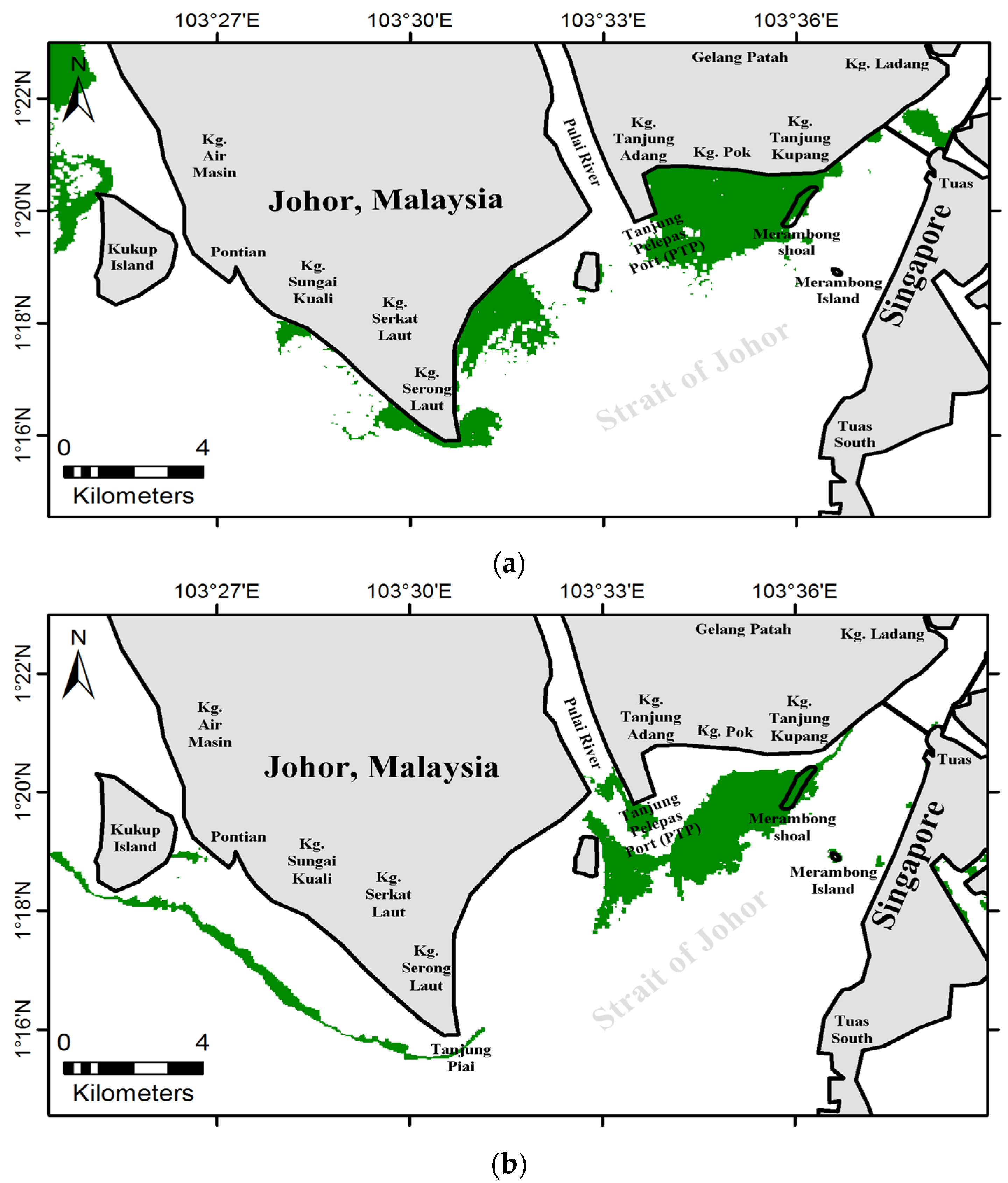
3.1. Changes on the Seagrass Distribution Map between 2009 and 2013 in the Merambong Area

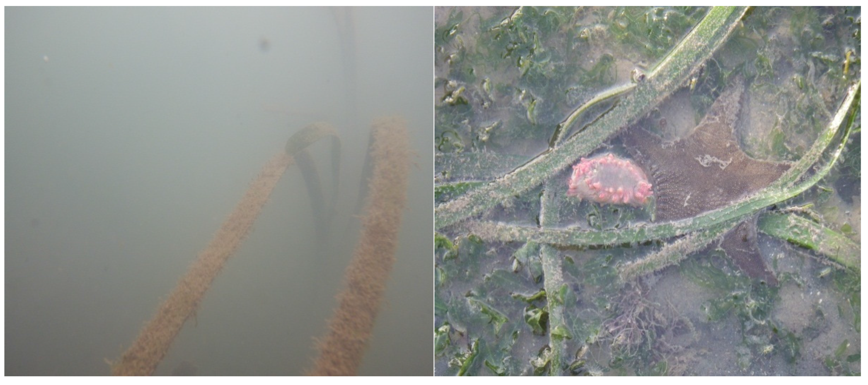
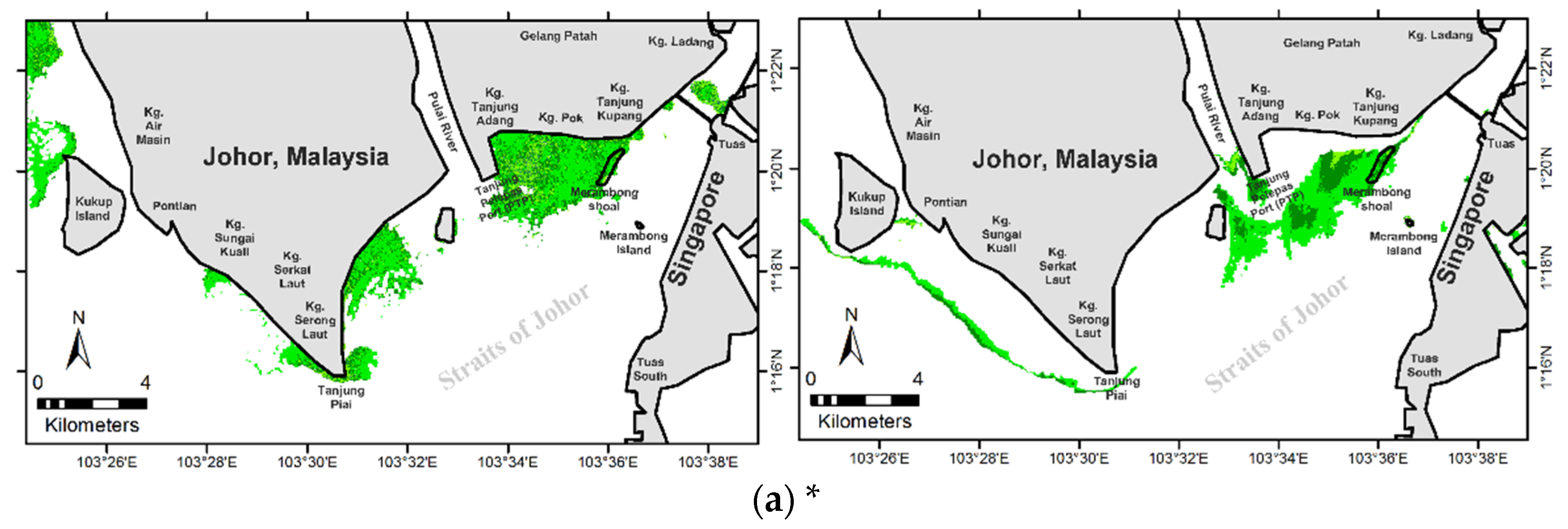
From Figure 7, it can be depicted that seagrasses around the Merambong shoal were submerged and could only be seen through diving. Intertidal seagrass data can only be collected during low tides.

Table 7. Summary of submerged seagrass area by MLC.

Class	Landsat 5 TM (2009)	Landsat 8 OLI (2013)	Changes
			Status	Percentage Changes
Mud	15,546.9 km2	14,637.5 km2	Decrement	−5.8%
Seagrass	23,377.8 km2	14,773.5 km2	Decrement	−36.8%
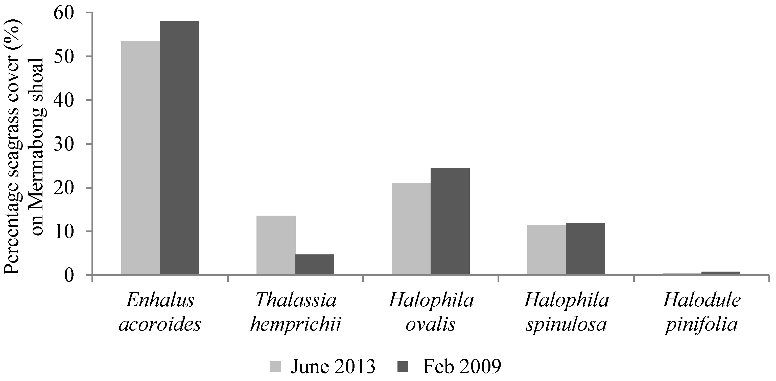
Deep water	15,562.0 km2	25,058.7 km2	Increment	+37.9%

tabulates seagrass changes over the study period.

Peninsula of Malaysia is exposed to two types of monsoons: (a) northeast monsoon (November–March) and (b) southwest monsoon (April–October). These seasonal changes are more apparent during transient periods (December and January), which causes severe impact of annual floods in many states of Malaysia Peninsula, especially the eastern region. Seagrass habitats along the Straits of Johor become vulnerable due to the southwest monsoon. However, the Sumatera Island reduces the wind velocity, evades extreme speed of water current towards the confined areas of Merambong and often causes uprooting of seagrass roots from the ground [35,36], especially to the Halophila ovalis. However, the impact of monsoon seasons on seagrass growth and decrement is not significant and prominent due to areas being sheltered by Malaysia Peninsula and Singapore Islands, located in both north and south, respectively.

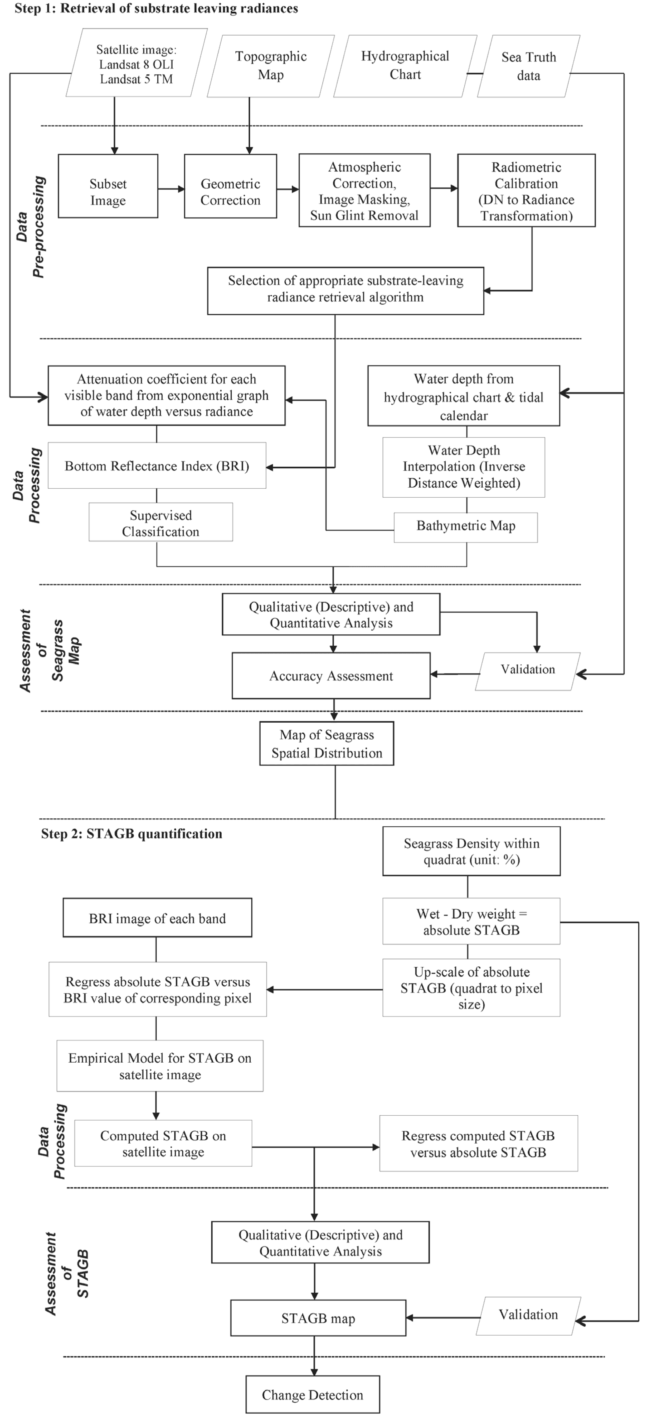
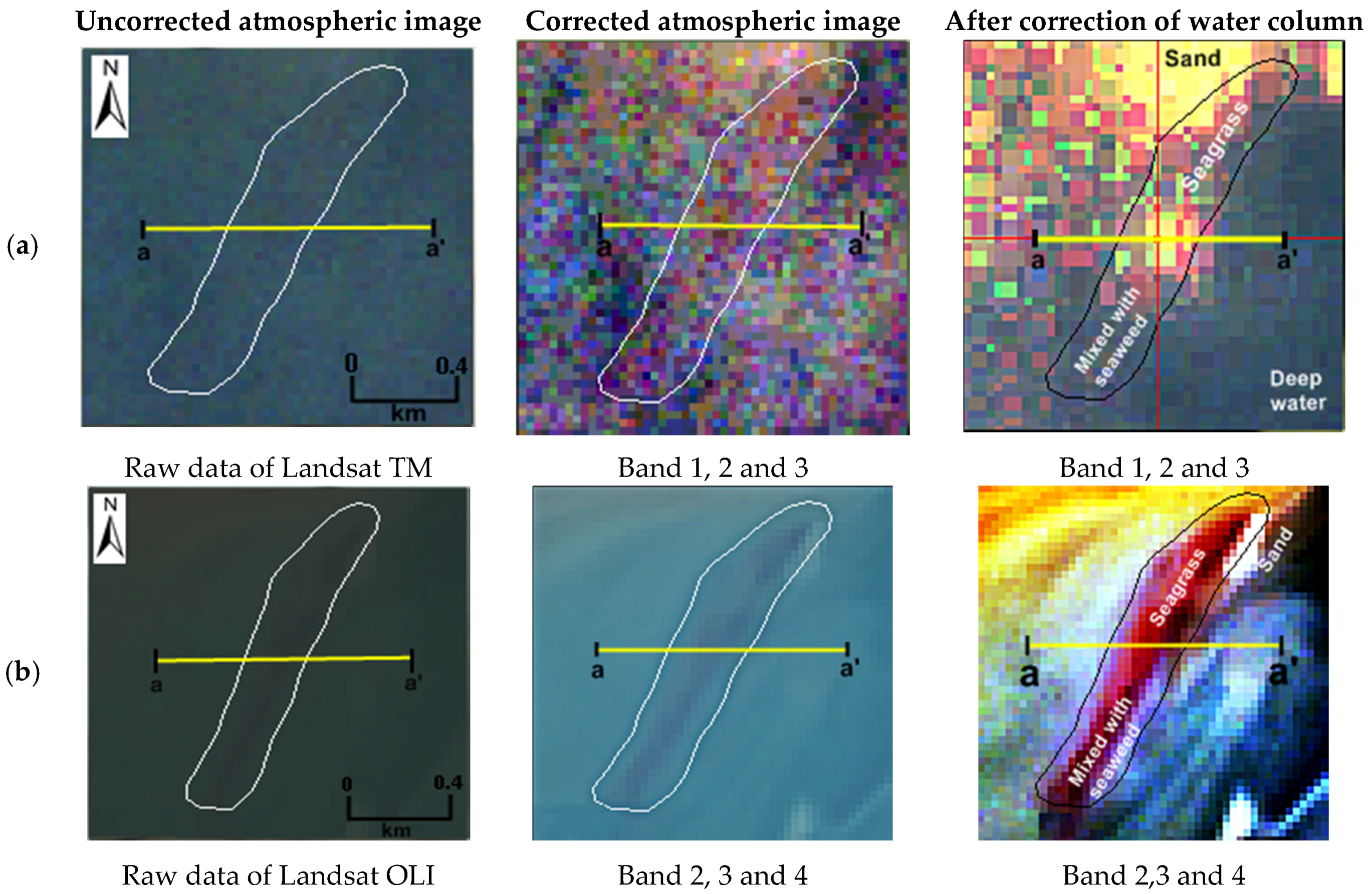
As mentioned earlier, blue and red bands were used in this study because blue bands have better water penetration ability compared to others, while the functionality of green bands are similar to blue bands but not as good as the blue bands. The coastal aerosol band of Landsat 8 OLI, which has more powerful penetrative power than the blue bands, was not used in this study because the assessment of the result is based on the common corresponding wavelength of both satellite data. Red bands were also used to derive BRI and are highly sensitive to changes in reflectance which is radiated back from seagrass. Under such a condition, the heterogeneous nature of substrata, low reflectance signal and greater light attenuation that varies with depths in less clear water may lead to misclassification, especially in the case of detecting small patches of seagrass where there are high similarities of signal response between seagrass and seaweed at coarse spectral resolution of Landsat. The results indicate good agreement with in situ validation test results. The seagrass occurrence areas were classified with 79.5% and 85.9% overall classification accuracies and, 0.7975 and 0.8104 kappa coefficients for Landsat TM and OLI, respectively.

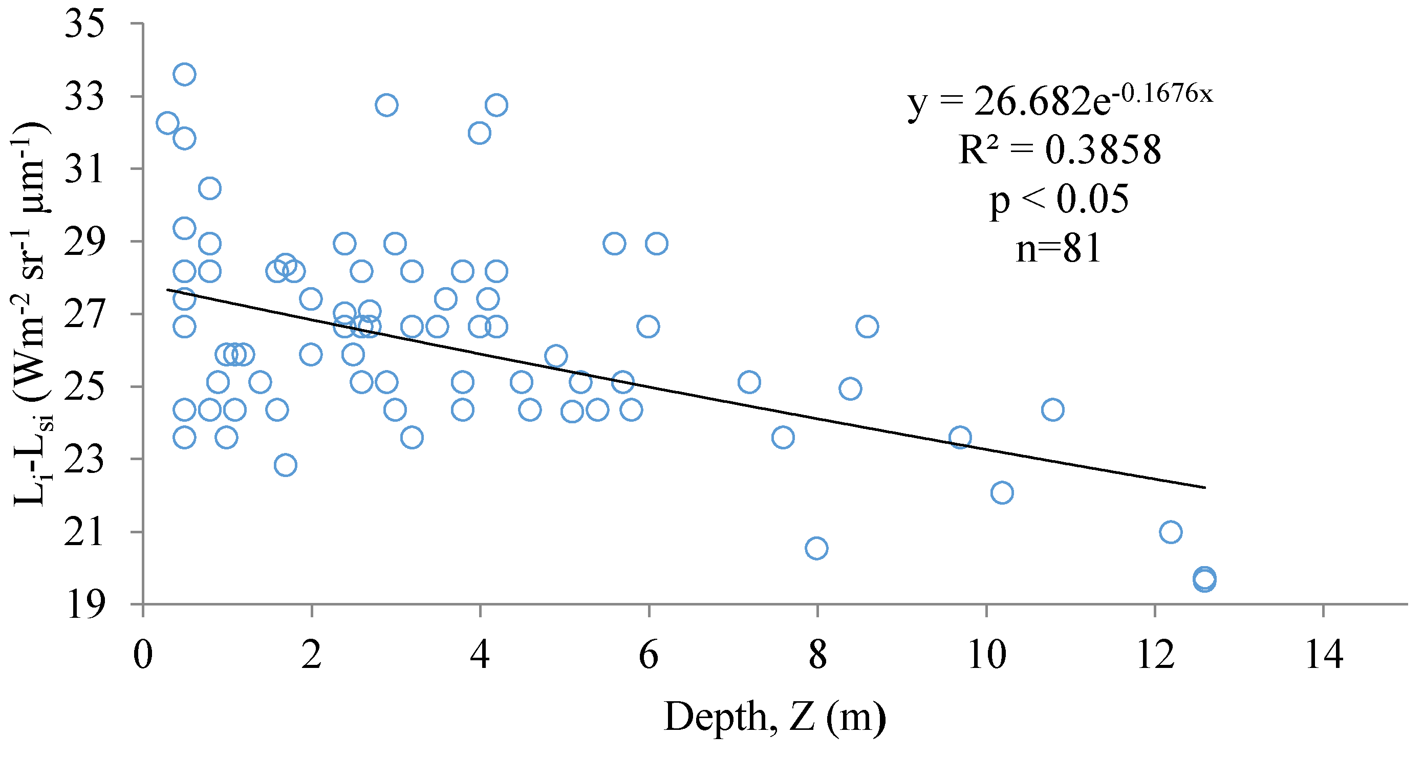
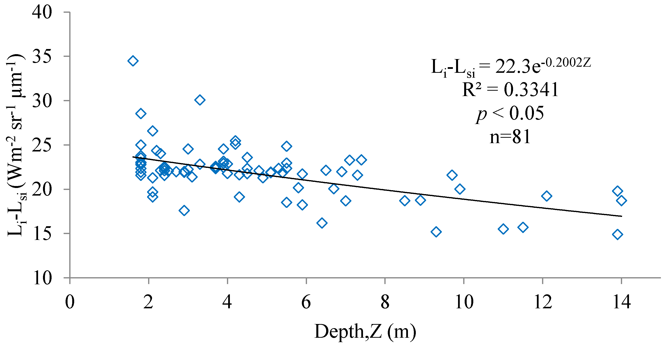
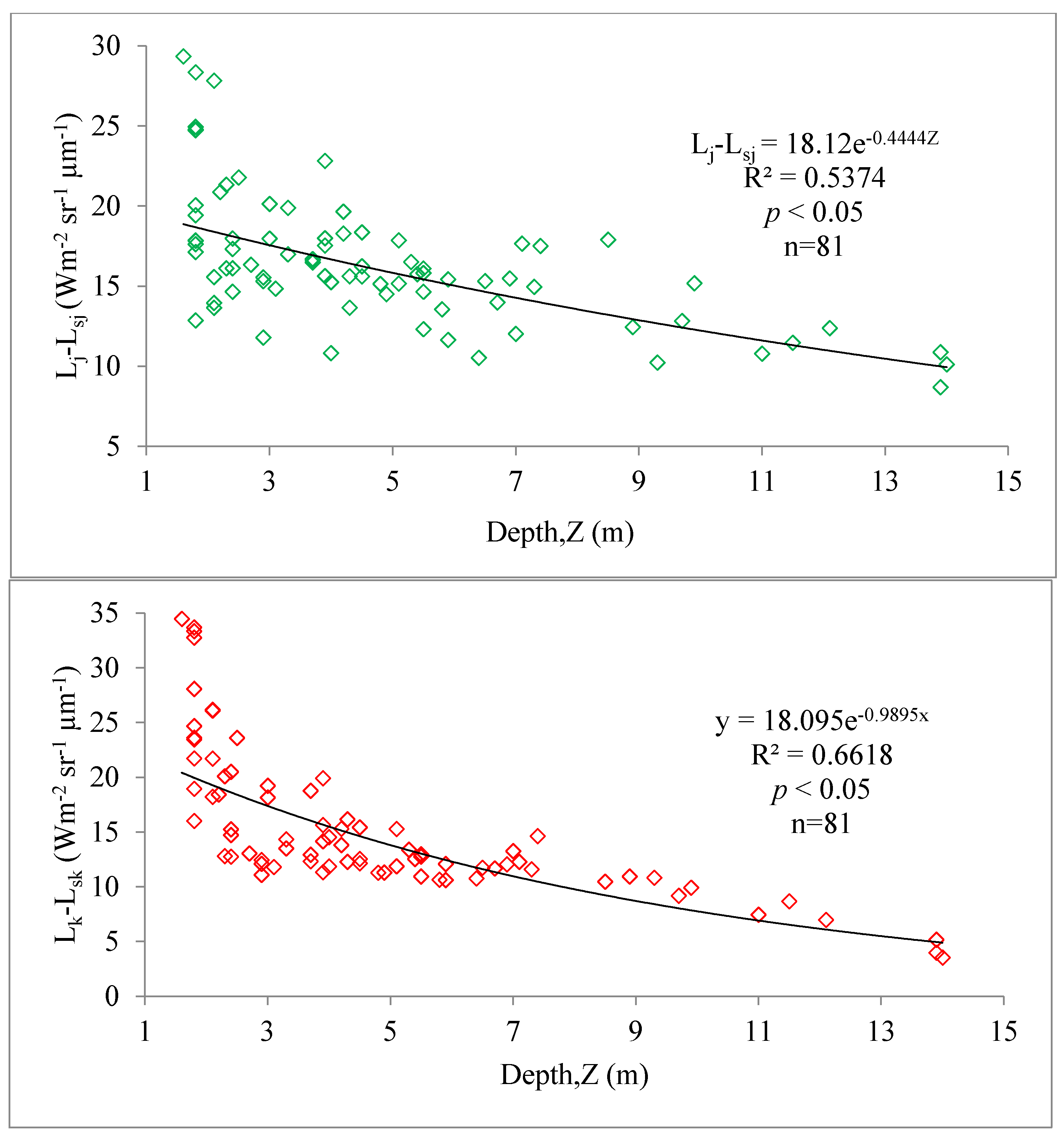
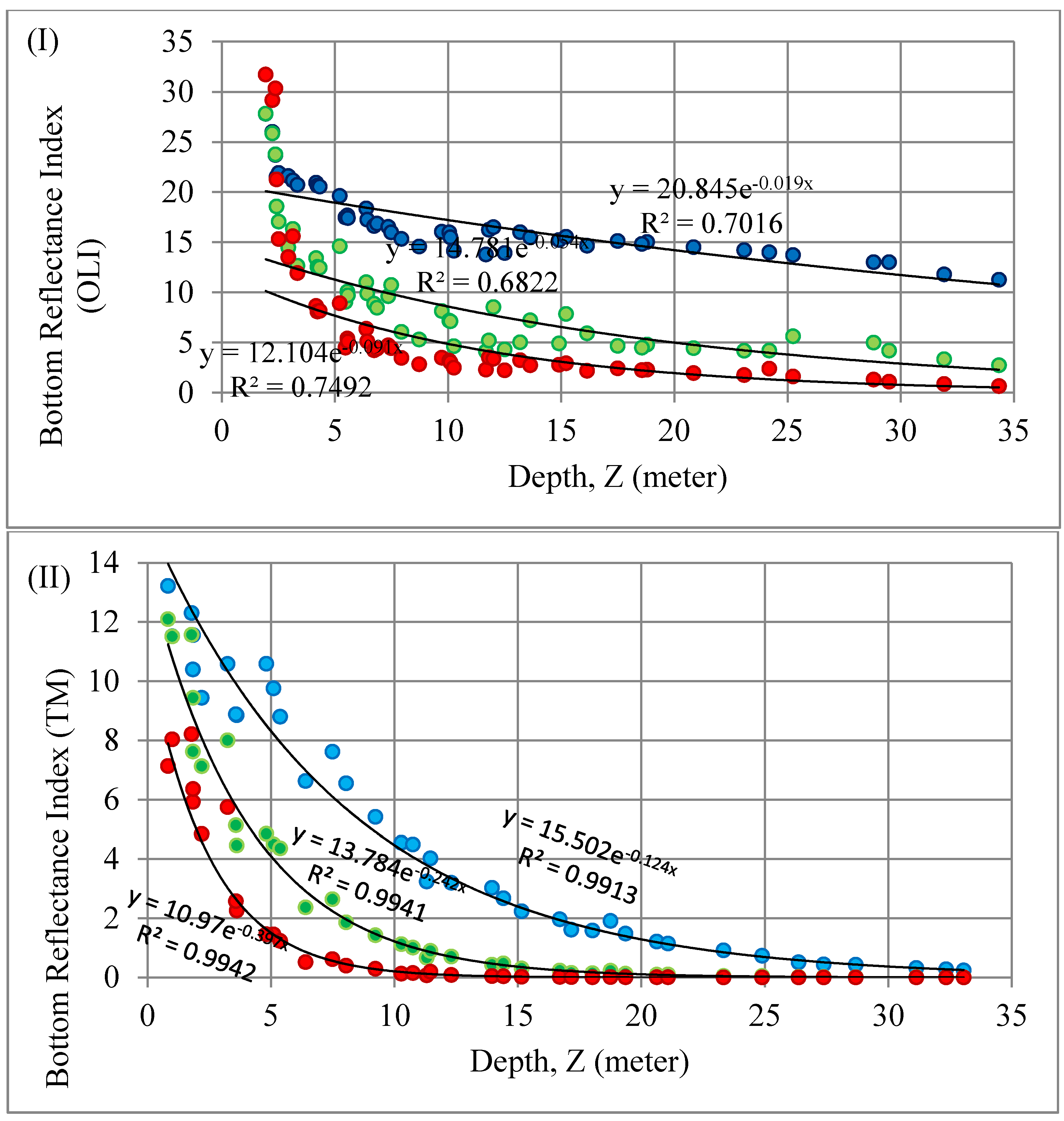
When submerged seagrass vigorously grows at various densities, the corresponding reflectance is affected by the water body and thus water column correction is necessary. Based on the result, the top of the BRI equation (L_i − L_si) shows an exponential relationship between corrected radiance with increasing water depth. It illustrates that substrate-leaving radiance received by the satellite sensor decreases with increasing water depths due to light attenuation. Blue bands of both Landsat TM and OLI images are able to receive more accurate bottom reflectance than other visible bands. This trend is shown on Landsat TM and OLI using BRI at a non-ideal condition of water clarity at various depths in the Merambong area (Appendices A and B).

From visual inspection, bright BRI pixels indicate medium to low density seagrass coverage and dark BRI pixels indicate high density seagrass after masking out non-seagrass pixel. Before masking out non-seagrass pixels, BRI for sandy area is even brighter and deep water pixels are dark in color, especially at red bands where reflectance from sea bottom surface is almost zero due to its signal incapability to reach and detect features above the sea floor, only at air–water surface to a few millimeters of penetration only (Appendices C and D).

In addition, nutrient load in turbid water, however, is relatively high in seagrass areas near the estuary and subject to rapid changes in its concentration. These nutrients are originated from the terrestrial sources through water channels and consumed by many marine creatures and aquatic plants. There are more than 150 active local fishermen that live along the riverside of Pulai River. Hence, collective nutrients dissipated from food waste, human daily disposal as well as suspended sediment are directly channeled through river flows and reach seagrass habitat. This might have enhanced growth, stimulated flowering, and has resulted in high density seagrass coverage in 2009, about four years after accomplishment and extension of Tanjung Pelepas Port (PTP). In fact, the part of the Merambong shoal that face off the PTP at this time has high STAGB and less bared sand areas.

In 2013, the significant increase of shipping traffic to PTP had caused increased oil spill from the huge ship and had made seagrass growth and survival vulnerable, which is opposite to the seagrass growing condition in early 2009. Massive pollutants such as toxic chemicals from the expanding number of peoples living along the coastline of Kg. Pok, Kg. Tanjung Adang and Kg. Serong Laut may have indirectly diminished the seagrass coverage, retarded shoot regeneration and thus decreased STAGB. The dynamics of seagrass spatial extent, coverage density and shoot density are the important factors that influence the significant changes on the seagrass biomass [37]. This is supported by the statistical report of the local government agencies that stated soil loss from 2009 to 2013 in this area, which increased due to erosion caused by wave speed from the sea [8]. The impact of sea currents to the shore with high speeds could be beyond the tolerance of seagrass. Seagrass coverage in this area were dwindling due to these factors as well as hectic trade shipping routes from and to the port that threatened seagrass habitat and subsequently decreased STAGB. As a result, the variation of BRI range on seagrass habitat can represent pixel-based quantification of submerged STAGB at various densities in near-turbid water where human-induced disturbances are prime contributing factors to its loss and coastal ecosystem imbalance.

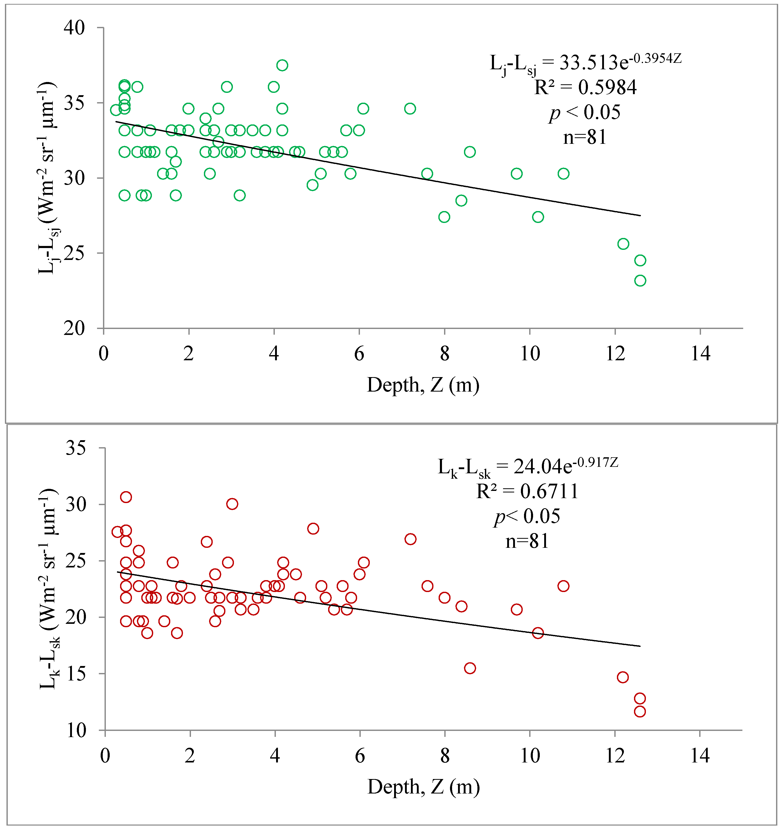
The relationship between water leaving radiance of visible bands and bottom depth at visible bands (n = 81, well-distributed) shows that the Landsat 5 TM image has better correlations compared to Landsat 8 OLI for all visible bands. It might be due to low water tide condition when the scene was acquired on 8 February 2009 (+0.19 m) as compared to the scene acquired on 27 June 2013 (+1.50 m). This condition significantly enhanced the capability of BRI to detect seagrass effectively and was also due to low Nephelone Turbidity Unit (NTU), which indicates the turbidity level, measured by WQC during this time compared to NTU of water in 2013. Red bands showed high correlation with depth at the Merambong area because of its inability to penetrate deeply into the column of turbid water as shown by highest Attenuation coefficient, K_i value compared to green and blue bands, meaning that it is almost perfectly absorbed at the deeper region. Sensitivity of spectral bands of Landsat 8 OLI was higher than Landsat 5 TM because the OLI sensor has higher quantum level and wider range of radiometric scale than TM. From this, BRI range is efficiently effective for STAGB quantification on multispectral bands after performing water column correction to solve ambiguity of bottom reflectance from less clear water.

The K_i of blue, green and red bands on both the images showed an increasing trend from shorter (blue band) to longer wavelength (red band) (

Table 8. Light attenuation used in water column correction on Landsat image.

Band (Landsat TM)	Attenuation Coefficient, Ki	Geometric Factor, g	Exponential Relationship of Depth and Corrected Radian	Determination Coefficient, R2
2009
Blue (Band 1)	0.0781	2.1456	Li − Lsi = 26.682e−0.1676Z	0.3858
Green (Band 2)	0.1843	2.1456	Lj − Lsj = 33.513e−0.3954Z	0.5984
Red (Band 3)	0.4274	2.1456	Lk − Lsk = 24.04e−0.917Z	0.6711
2013
Blue (Band 2)	0.0942	2.1253	Li − Lsi = 22.3e−0.2002Z	0.3341
Green (Band 3)	0.2091	2.1253	Lj − Lsj = 18.12e−0.4444Z	0.5374
Red (Band 4)	0.4656	2.1253	Lk − Lsk = 18.095e−0.9895Z	0.6618

). It indicates that light is quickly attenuated when it passes through the water column at longer wavelength. High K_i would decrease by capturing in chlorophyll pigments of seagrass leaves, reducing the detectability chances from Landsat. Blue bands (0.45–0.51 µm) have very good ability to penetrate into the water column in clear water and are still the best among other visible bands in context of its penetration ability into non-clear water for the areas (i.e., Merambong shoal). Based on Table 8, all these values are relatively smaller than the K_i of pure sea water, which are about 0.0064, 0.015 and 0.32 for respective blue, green and red bands. The smallest K_i of BRI are blue bands, followed by green and red bands susceptible to light attenuation for both 2009 and 2013 images. It means that this water is relatively transparent to the shorter wavelength (blue band) and seagrass patch and its density can be determined efficiently better than other bands. This trend is expected to be similar if BRI is applied on visible bands of other satellite imagery; light is highly attenuated in longer wavelength of visible bands (

Table 9. Deep-water statistics for Landsat 5 TM and Landsat 8 OLI visible bands.

	Blue Band		Green Band		Red Band
	TM	OLI	TM	OLI	TM	OLI
Minimum	65.6425	58.8487	51.8731	45.2182	30.8339	20.1162
Maximum	78.1637	70.7194	68.9461	58.53396	40.1194	38.6417
Mean	67.8431	61.8373	53.4066	47.2820	30.9440	22.1798
Standard deviation	3.5724	4.5876	2.1047	3.0164	3.2086	4.2246

). For this reason, blue bands are used for STAGB quantification in this study after implementation of BRI on both the images.

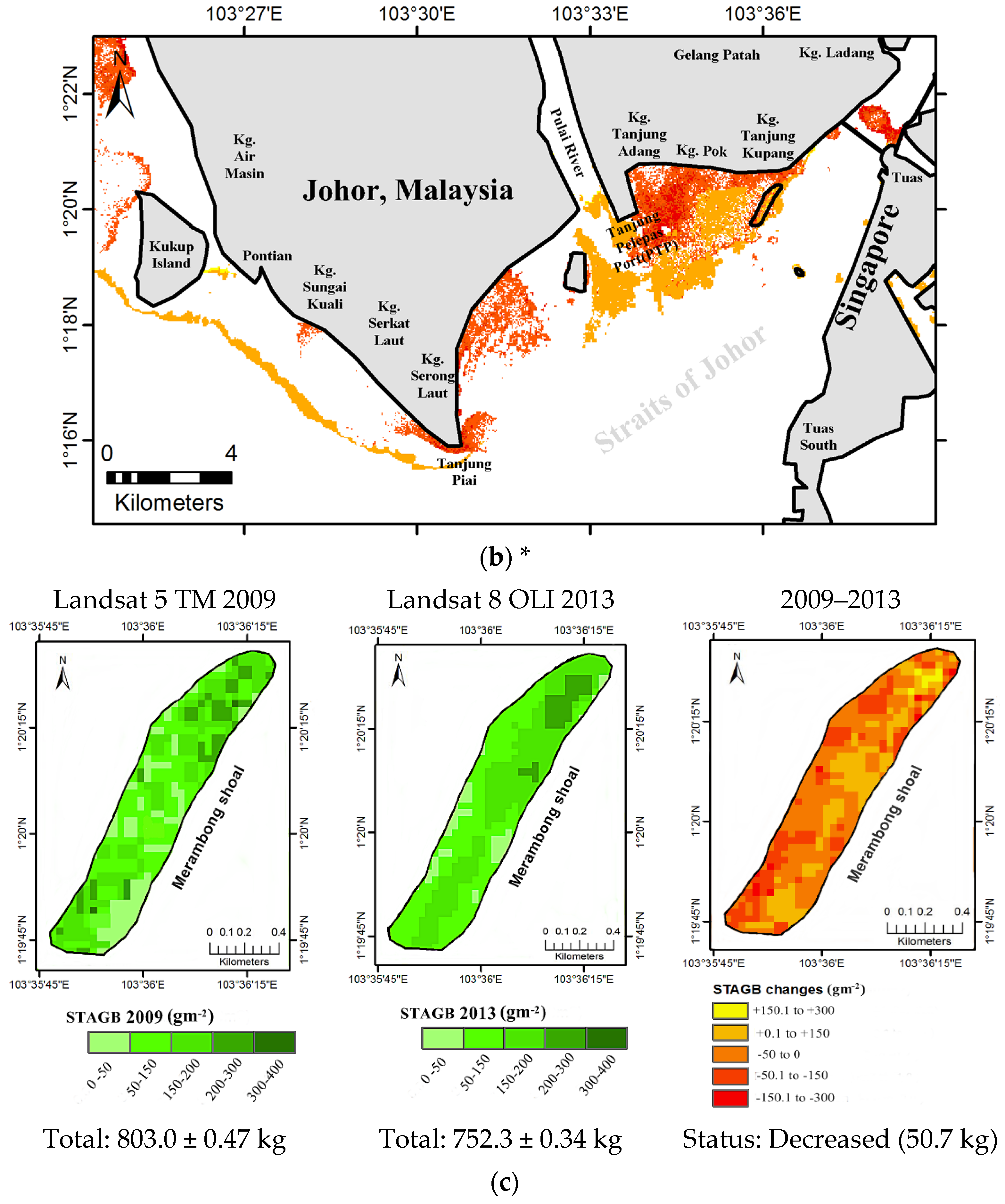
3.2. Changes of STAGB between 2009 and 2013 on the Merambong Shoal

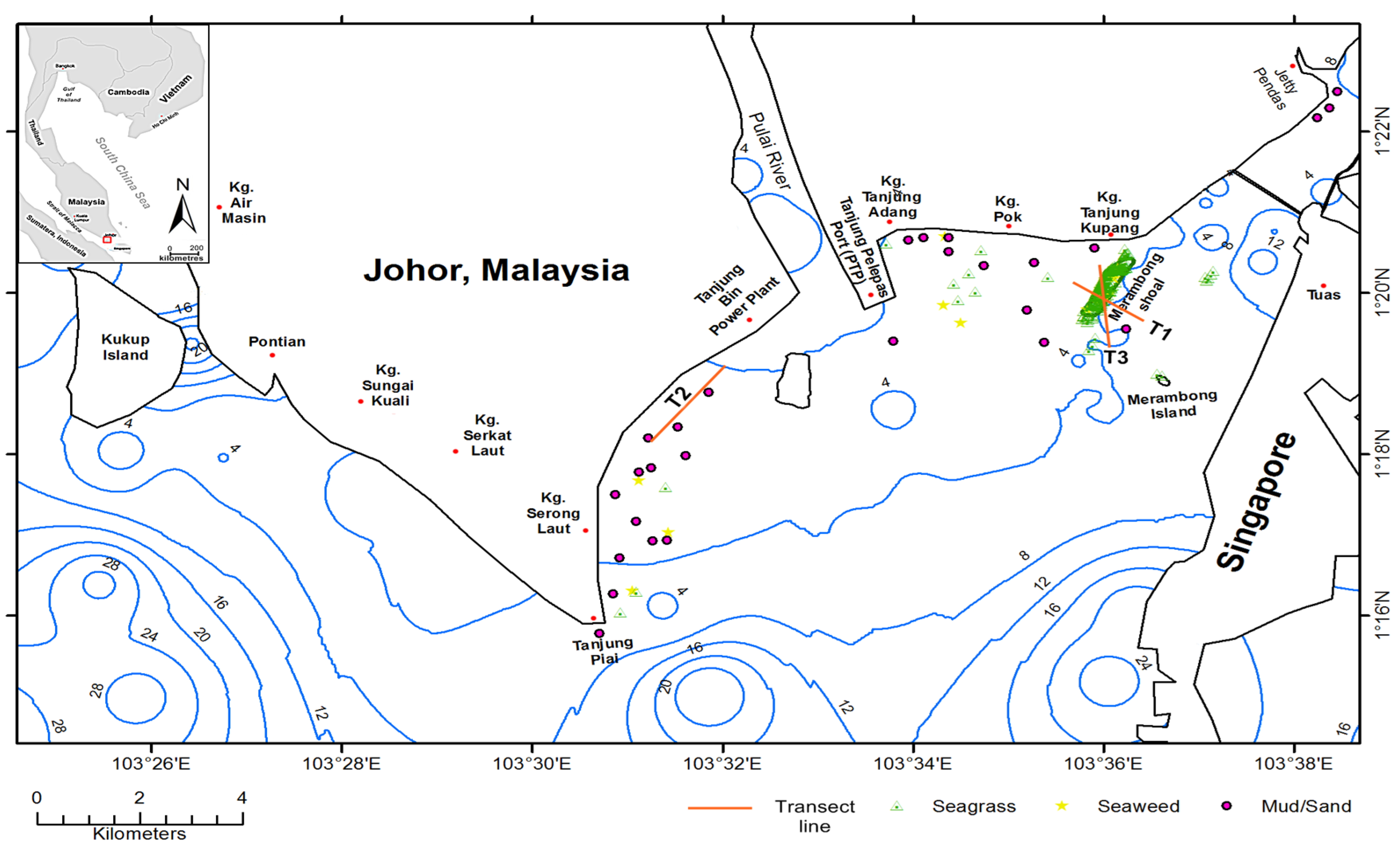
Apart from bigger area changes, this study also concentrated on the intertidal seagrass meadow, focusing on the Merambong shoal. Figure 8 shows the change analysis of submerged STAGB of Merambong shoal which was quantified from Landsat OLI data.

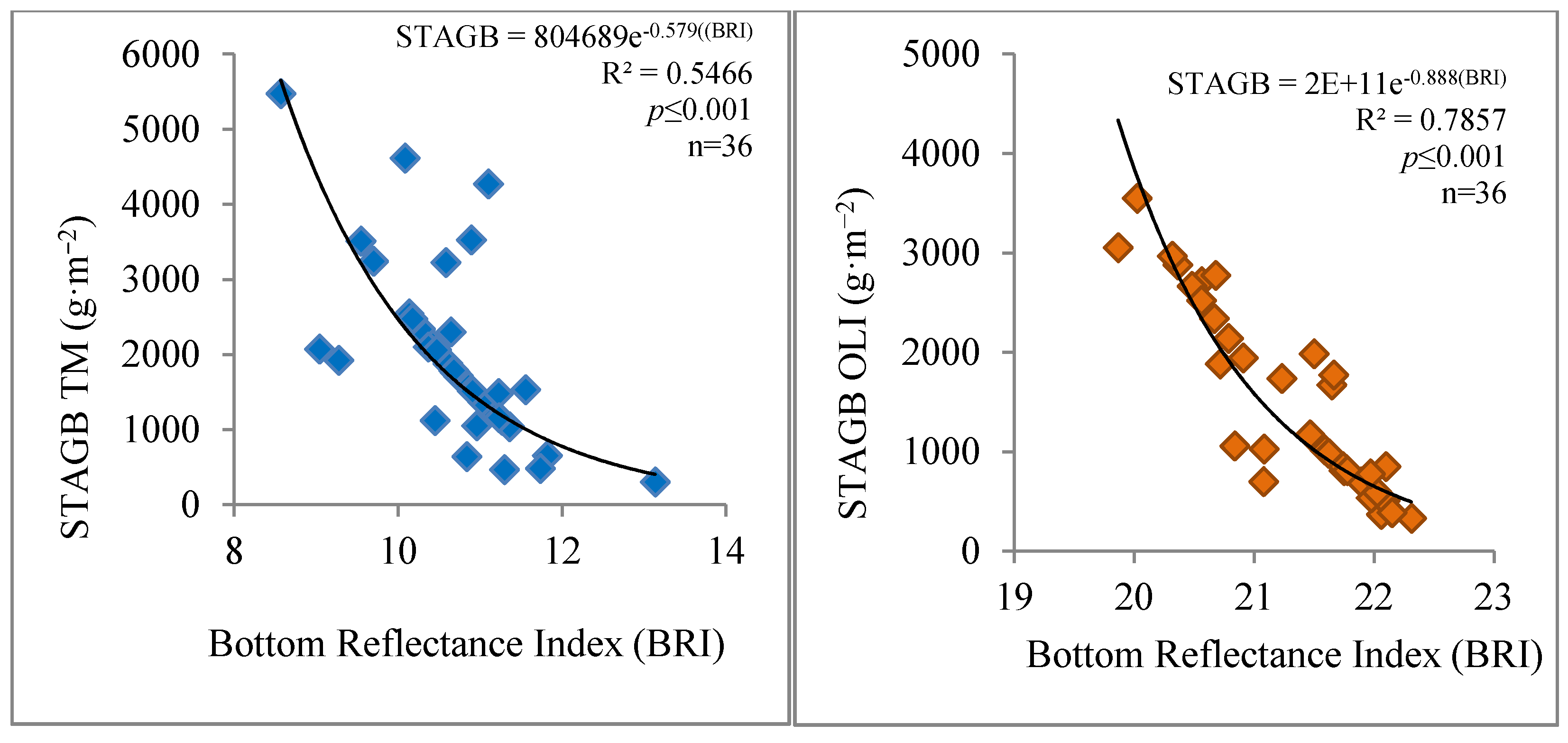
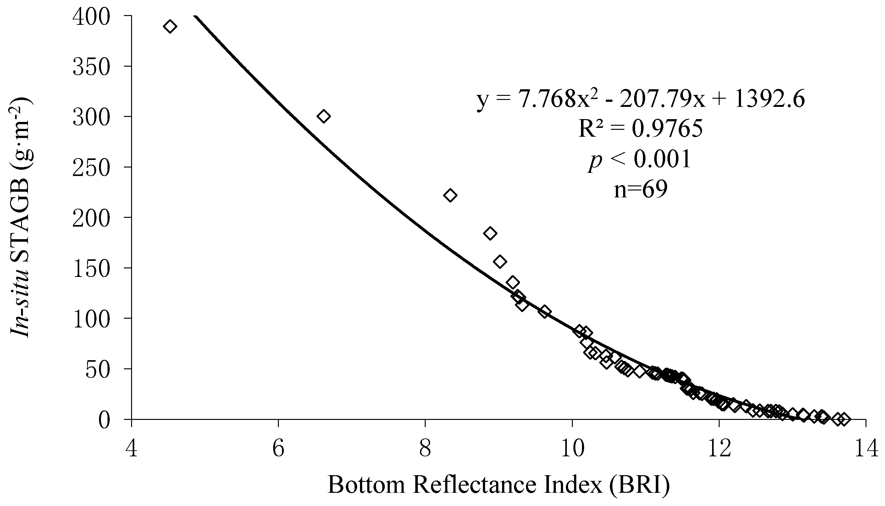
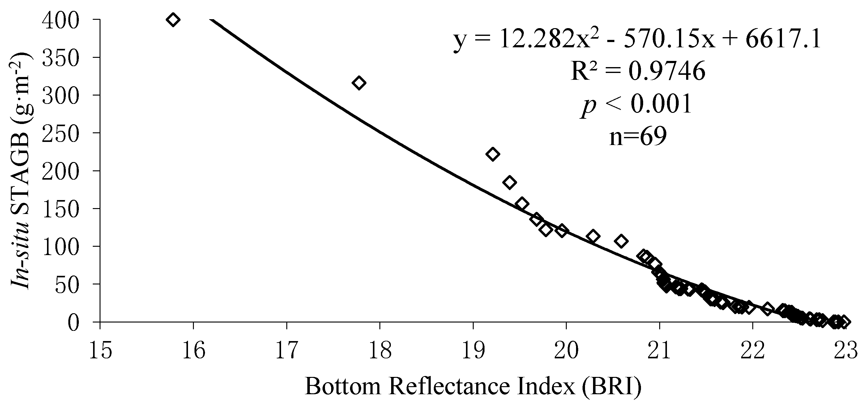
At the second stage of the study, an approach was devised to quantify STAGB based on the correlation of seagrass coverage and weight with the corresponding corrected substrate leaving reflectance or BRI. The relationship derived from in situ seagrass biomass and density coverage is very high, whilst the final BRI-seagrass biomass established for final empirical model for estimating seagrass biomass from satellite for the best bands (blue bands) is given in Figure 9 using another set of in situ for verification. The BRI of seagrass dominant pixel is relatively higher than previous study conducted by [19] in clear water. This indicates that the effect of high light scattering amount of total suspended sediments in water could increase BRI value of seagrass detected pixels due to low attenuation coefficient.

The classification results were extended to be used for STAGB quantification. Since BRI_b,r shows the most accurate results of the seagrass distribution map, corresponding spectral response of the BRI of blue bands (BRI_b) and red bands (BRI_r) is regressed with STAGB quantified in the laboratory. The BRI_b shows higher correlation coefficient (0.5466 and 0.7857 for TM and OLI, respectively) than BRI_r (0.3782 and 0.5291 for TM and OLI, respectively). Hence, the next steps will focus on BRI_b of both TM and OLI only. Trade-off between spectral and spatial properties of Landsat 8 OLI images has shown relatively more accurate results of STAGB quantification that is very useful for coastal management if compared to previous series of Landsat imagery. The accuracy of STAGB remote sensing can be affected by many factors such as image resolution, water clarity, quality and algorithm, depth of seagrass distribution and density. In order to improve classification accuracy, in situ observation was checked with information from an underwater camera as a supporting input for seagrass detection and its coverage on BRI of Landsat data. Moreover, the background of the seafloor was also an important factor in achieving good results that affect STAGB accuracy level. Sediments of Merambong area are mainly comprised of sand and mud, which makes it relatively easier to quantify STAGB by the remote sensing approach.

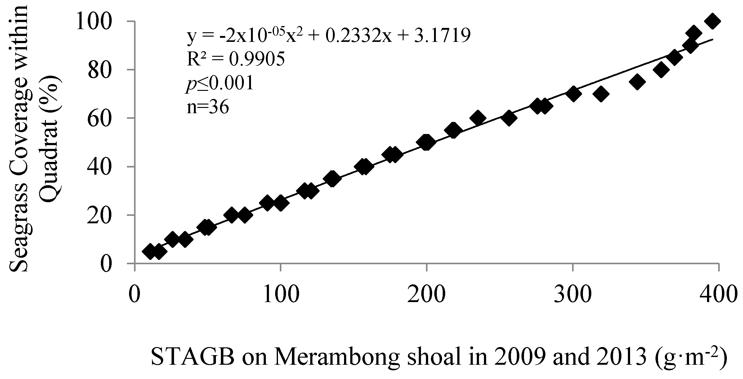
The regression analysis was done to create a STAGB map on both scenes and finally detect the changes occurred within the study periods. The regression graphs are developed based on the following steps: (i) seagrass coverage versus STAGB measured in the ground or laboratory; and (ii) BRI_b versus STAGB in the ground or seagrass coverage. The results of the STAGB regression analyses are shown in Figure 10, and the transects analysis is summarized in

Table 10. BRI variation of two bands along few transects as shown in Figure 1 across the different sea bottom features. The left column is for Landsat 5 TM 2009 and the right column is for Landsat 8 OLI 2013.

Transect 1 (seagrass → deep water)
Transect 2 (mud → seagrass)
Transect 3 (mud → seagrass → deep water)

.

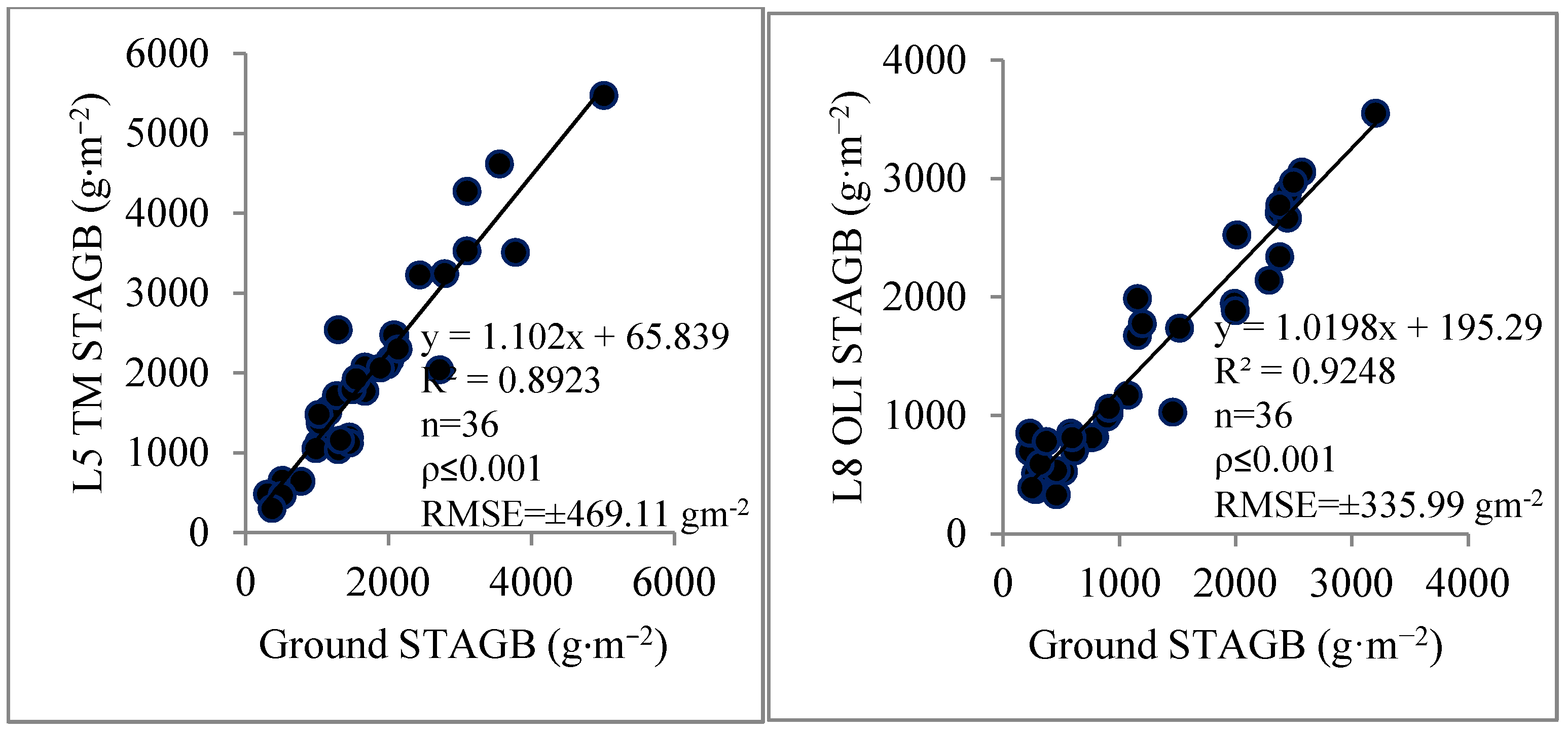
In this study, STAGB measured in the ground and STAGB predicted from BRI has been compared. The result shows that BRI_b derived from Landsat OLI is slightly higher than TM even the seagrass coverage is similar (

Table 11. Results of seagrass total aboveground biomass (STAGB) with respect to BRI range.

Seagrass	BRIb	BRIb	STAGBGround (g·m−2)	STAGBLandsat (g·m−2)
Coverage (%)	TM	OLI
0–20	13.8–12.8	23.0–21.1	0–80	0–90.5
20.1–40	12.7–11.2	21.0–19.2	80.1–155	90.6–160.5
40.1–60	11.1–10.2	19.1–18.2	155.1–250	160.6–274.1
60.1–80	10.1–9.6	18.1–17.0	250.1–350	274.2–368.8
80.1–100	9.5–9.0	16.9–15.9	350.1–400	368.8–400

), which might be due to influence of higher quantum level of Landsat OLI and water quality. Moreover, it seems STAGB measured from remotely sensed images overestimated the biomass matrices compared to manually measured STAGB. Determination coefficient, R² from regression plot in Figure 11 between STAGB measured from ground with STAGB quantify from both images is high, 0.92 and 0.89 for Landsat OLI and TM, with respective RMSE ± 469.11 g·m⁻² and RMSE ± 335.99 g·m⁻² for each 30 m pixel resolution.

Compared to other seagrass habitat around Malaysia Peninsula, the Merambong shoal is a better place for comparison of submerged seagrass occurrence change analysis and demonstrating STAGB changes in Case-2 water using satellite remote sensing data due to its accessibility, multi-species of massive submerged seagrass and satellite data availability. Since the Merambong coastal area is closely surrounded by land, the changes of STAGB can be effectively detected from the satellite data after few years interval. Satellite remote sensing data in different monsoon seasons of late northeast Monsoon season of 2009 and middle southwest Monsoon season in June 2013 were used for STAGB change comparisons. Absence of major natural disturbances such as hurricanes and tsunami, temporal variations in submerged seagrass distribution and the STAGB changes in these tropical environments are expected to be minimal. Seagrass patches vary in size and density around this shoal. The substrate is comprised of unconsolidated soft sediments, including muddy to shelly sands with occasional hard bottom substrates. Seagrass meadows are being negatively affected by pollution (pollutants may include herbicide runoff, sewage, detergents, heavy metals, hypersaline water from desalination plants, and other waste products), algal blooms and high boat traffic. All these pressuring factors have catalyzed the decrement of STAGB tremendously [9].

Furthermore, the result shows overestimation of seagrass extent on both the images where sparse to moderate percentage of seagrass cover was assumed to be continuous seagrass area. This is clearly seen at certain pixels when overlaid with in situ data collected at the study area, where overestimation (±30%) on Landsat 5 TM is higher than Landsat 8 OLI (±10%). Such estimation possibly comes from different radiometric resolution, Landsat TM which has only 8-bit (DN range: 0–255) compared to Landsat 8 OLI with 65,536 grey levels on each pixel (DN range: 0–65,535). It was expected that the variability of STAGB changes would not successfully be reported in less clear water due to high sedimentation concentration. However, the results prove contradictory as this technique revealed that the changes that occur coincide with STAGB quantified manually in the laboratory at specific selected locations. In the selection of the most appropriate model to quantify STAGB, determination of coefficient from regression analysis was used as the main indicator. The list of the regression model is tabulated in

Table 12. Regression models of STAGB versus BRI derived with TM and OLI.

Regression Model	Equation	R2
Landsat TM: Linear **	STAGB = −940.75BRI + 12055	0.44
Logarithmic **	STAGB = −9986ln(BRI) + 25628	0.44
Polynomial (second order) *	STAGB = 67.818BRI2 − 2389.1BRI + 19741	0.44
Power **	STAGB = 2E + 09BRI−5.987	0.52
Exponential ***	STAGB = 804689E−0.579(BRI)	0.55
Landsat OLI: Linear *	STAGB = −1241.3BRI + 27941	0.83
Logarithmic ***	STAGB = −26292ln(BRI) + 81908	0.83
Polynomial (second order) ***	STAGB = 170.73BRI2 − 8471.3BRI + 104405	0.85
Power *	STAGB = 9E + 27BRI−18.74	0.78
Exponential **	STAGB = 2E + 11e−0.888(BRI)	0.79

Note: significant levels: * p ≤ 0.05; ** p ≤ 0.01; ***p ≤ 0.001.

. Thus, the exponential model is the most fitted model for STAGB derivation on Landsat 5 TM, and the polynomial second order model is the most suited to be used on Landsat 8 OLI.

Merambong shoal and its vicinity is densely covered by Ea, STAGB quantification of STAGB in this area was expected to produce high content of aboveground biomass. For Landsat 5 TM in 2009, submerged STAGB was quantified using this empirical model,

STAGB_TM = ae^−b(BRI)

(6)

where a = 804689; and b = 0.579.

Since the correlation coefficient (R²) of this model shows moderate degree of correlation with BRI of the satellite image processed (0.50466), the submerged STAGB is considered acceptable for 30 m pixel of Landsat with 8-bit quantization level. On the other hand, the empirical model for Landsat 8 OLI 2013 is

STAGB_OLI = aBRI² − bBRI + c

(7)

where a = 170.73; b = 8471.3; and c = 104405

For the equal parameters, BRI of Landsat 8 OLI seems better to quantify STAGB at such water clarity, indicated by R² = 0.7857 and significantly different, p < 0.001. This may the ability of the image with 16 quantization level (DN range 0–655535) to quantify STAGB from BRI range; in fact, to discriminate seagrass among the other bottom features as well as has good exponential relationship between depth and attenuation of coefficient (see Figure A1 and Figure A2), compared to Landsat 2009. From the regression graph, although BRI of Landsat 5 TM had very good correlation with depth, in terms of STAGB mapping, Landsat 8 OLI showed greater accuracy and higher correlation to STAGB measured on the ground (refer to regression graph of STAGB satellite versus in situ STAGB, see Figure A3). Based on this result, it can be stated that Landsat 8 OLI with higher radiometric resolution has better conformity with BRI to quantify submerged STAGB and yielded better result accuracy than TM.

BRI conformity derived from Landsat 5 TM bands 1, 2 and 3, and Landsat 8 OLI bands 2, 3 and 4, were the best in terms of significant trends of L_i − L_si plotted against the depths, and deriving the attenuation coefficients at any respective bands. The evidence of the best to fair applicability of BRI was derived using blue, green and red bands, respectively. The attenuation coefficients obtained for the blue, green and red bands for coastal Case-2 coastal water of Merambong shoals and its vicinity were 0.008,0.016 and 0.027, for respective bands in 2009, and a slight increase in 2013 where they were 0.009, 0.026 and 0.047, respectively. These values are within expected range in such turbid water [20,35], i.e., the shorter blue bands having the least attenuation coefficient for deeper penetrable power. Subsequently, this sequence is followed by green and red bands with less and the least penetration power, respectively (see Figure A4).

The final seagrass aboveground biomass map for both dates on the entire Merambong shoal at Straits of Johor is shown in Figure 8, mapped with a total of 411 BRI pixels where each pixel is 900 m², yielded a total area of 5.677 ha. The STAGB of Merambong shoal at the end of June 2013 estimated a total above ground biomass of 752.1 kg, with range between 0.5 g·m⁻² and 380 g·m⁻². This amount shows a declination trend compared to 2009 where the STAGB was 803.0 kg, with range between 0.6 g·m⁻² and 382 g·m⁻². Hence, the average of pixel-based STAGB of Merambong shoal is 142.14 kg and 132.45 kg, respectively.

In a future prospectus, the method suggested by [16,38] should be explored for similar purposes in turbid water and allometric or physical-based model for submerged STAGB quantification comprehensively. By knowing the physical information of the submerged during the submerging satellite image acquisition, the forest biomass, using the allometric model [39], might be possibly integrated to quantify seagrass biomass in clear and less clear water. This work will help to sustain coastal sustainability and indirectly reduce the impacts of global climate change as reported by [40,41]. After this study, future research dictates that coastal aerosol band could be explored whether using this technique employing coastal aerosol band could improve accuracy results. With all the assumptions stated in the introductory section, STAGB changes over less tropical coastal water can be conducted with satisfying outputs.

Furthermore, applying this technique to different climate regions that experience significant seasonal changes of weather and temperature around the year to investigate the STAGB variations with other processing techniques. In addition, hyperspectral images such as Hyperion and ALI and high spatial resolution satellite images such as Worldview-3, Pleiades, Quickbird and GeoEye-2, compare with results shown in this study and enable species-based STAGB quantification in a non-ideal coastal water environment similar to the Merambong area.

Water quality plays an important function in the seagrass growth [38] and STAGB quantified on Landsat. The dynamics of seagrass recovery and declinations depends on water quality as well. To investigate the trends of STAGB declination, the water quality parameters between 2009 and 2013 were compared, and presented in

Table 13. Measurement of water quality parameters at 36 points on Merambong shoal and vicinity.

Parameter		Temperature (°C)	pH	Conductivity	Turbidity	Dissolved	Total Dissolved	Salinity
				(mS/cm)	(NTU)	Oxygen (mg/L)	Soild (mg/L)	(ppt)
Mean	2013	30.03	7.96	41.01	15.09	4.72	25.14	26.17
	2009	30.21	7.24	38.70	13.51	6.41	23.54	25.44
Minimum	2013	29.32	7.72	36.10	4.50	3.53	22.90	22.10
	2009	29.51	7.03	33.20	2.90	4.06	19.80	21.60
Maximum	2013	31.42	8.13	43.10	46.60	8.53	26.30	27.70
	2009	30.55	7.89	41.80	45.10	9.73	25.10	26.40
Standard deviation	2013	0.47	0.08	1.44	7.41	0.88	0.64	1.17
	2009	0.39	0.01	0.45	6.21	1.20	0.31	1.04

. Values represented by WQC confirm and support the idea that seagrass biomass is highly correlated with the clean environment.

This study is important to bring a significant impact to three main sectors: society, industry and environment. It is important to the group of people who depend upon the coastal resources including fisheries, mangrove forest, tourism as well as management authority of the coastal environment and the biodiversity of the marine life itself to know how the food security can be sustained at Merambong area since seagrass is the nursery and the primary food course for other organisms within the food chain. As the study states that about 50.7 kg biomass was lost within four years, possibly this trend could be worst in parallel to the rate of development and sand reclamation along the coastline, not including shipping traffic nearby Singapore and Johor port as well as sediment brought from river discharge through Pulai River. In fact, development in coastal regions may bring harm not only to seagrass but also coastal sustainability. However, the impact of the coastal landscape development is mild to coastal habitat. Most importantly, this study can be one of the indicators in assuring the status of coastal sustainability besides considering water quality changes, the rate of erosion on mangrove forest and fish catchment, and mitigation for future environmental threat since the area is become more actively developed as reclamation of seagrass habitat become prominent, based on our field inspection and worrying scientist on what are the significant changes that they will bring in and how to encounter this challenge so that marine life—especially species that live on seagrass bed like pipefish, seahorse, sea turtle, dugong and sea cucumber—can survive for preservation and conservation, at least to avoid drastic decline of their population along Johor Straits.

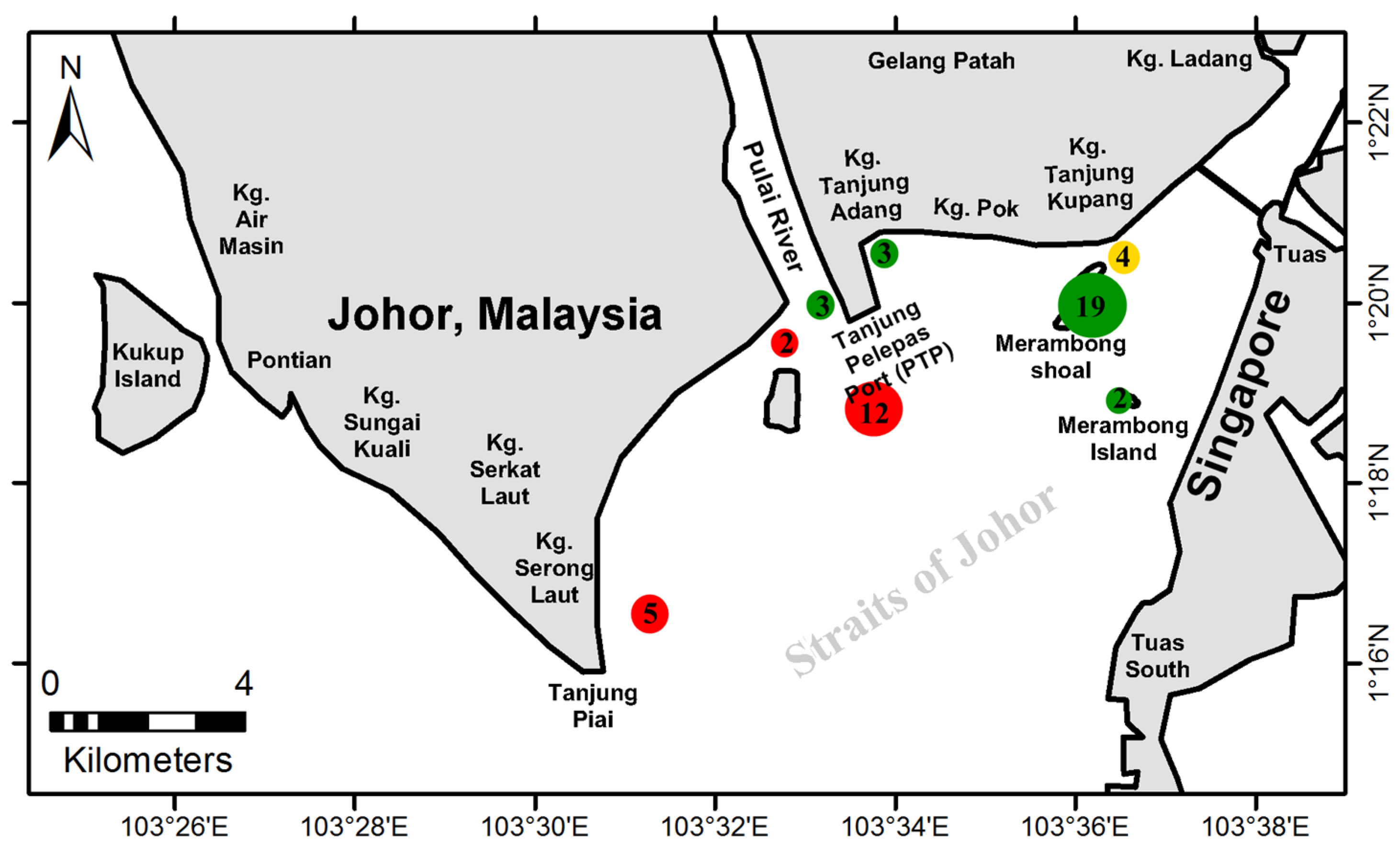
In addition, the STAGB map was correlated with dugong sighting frequency. We implemented an interview-based approach to survey the sighting frequency and the location of dugong (Dugong dugon), a sea mammal found in the respective area with seagrass as the main diet. The survey was conducted involving 60 local fishermen who were inhabitants of the Merambong coastal area (Pendas Jetty, Kg. Tanjung Adang, Kg. Pok, Kg. Serkat Laut and area of Tanjung Piai). However, only 31 (51.7%) among them had seen dugong from the years before 1999 to 2013. From this survey, it can be concluded that dugong was sighted more frequently at the Merambong coastline, especially Merambong shoal nearby Tanjung Kupang where high seagrass biomass is reported. The area nearby Tanjung Piai and Pulai River shows a decreasing number of dugong sighted, which started from 2000 to 2009 when the seagrass extent was declining. From 2010 to 2013, the area of dugong sighting shifted to an area close to Merambong shoal and PTP only as seagrass was shrinking. In this period, the number of dugong sightings increased due to spatial cover of seagrass remaining around this area only. Figure 12 summarizes the results of dugong sightings in the area.

In confirming the proportionality of biomass and dugong sighting, significant tests were carried out for to test the relationships between the decreasing trend of dugong sightings with decreasing mean of STAGB in this area. From the test, it was noted that they were significantly different (mean, t-test: p < 0.01), which shows that dugong appearance at this area is indeed highly dependent on seagrass biomass density in this area.

4. Conclusions

This study has successfully demonstrated the two-step STAGB mapping using appropriate processing techniques in a complex coastal environment. The robustness of BRI on a four-year interval of the Landsat image archive including Landsat TM and Landsat OLI imagery is validated. BRI was used to enable seagrass spatial distribution mapping in turbid water (great light attenuation vertically towards sea bottom) at Merambong area from two images of Landsat with a four-year interval due to hardly obtaining images with low cloud coverage in these tropical regions, dry and wet throughout the year. Sea truth information was used in training datasets in the classification scheme and validated the features.

The declining seagrass trend has possible connections to active human interferences and rapid coastal development along the coastline. However, some part of the seagrass bed shows recovery trends from 2009 to 2013 despite huge losses of seagrass biomass content occurring in the same habitat. Gradual changes in areas with high seagrass coverage and short term changes occurred in low seagrass coverage levels. With involvement of the field data set, the technique is validated and tested in a robust manner. To put it in a nutshell, BRI was not only limited to retrieval of water leaving radiances in seagrass identification, but was also capable of empirically quantifying STAGB in less clear water from satellite images.

References

1. Phinn, S.; Roelfsema, C.; Dekker, A.; Brando, V.; Anstee, J. Mapping seagrass species, cover and biomass in shallow waters: An assessment of satellite multi-spectral and airborne hyper-spectral imaging systems in Moreton Bay (Australia). Remote Sens. Environ. 2008, 112, 172–187. [Google Scholar] [CrossRef]
2. Ooi, S.J.; Kendrick, G.A.; Niel, K.V.; Affendi, Y.A. Knowledge gaps in tropical Southeast Asian seagrass systems. Estuar. Coast. Shelf Sci. 2011, 92, 118–131. [Google Scholar] [CrossRef]
3. Lyons, M.; Roelfsema, C.; Kovacs, E.; Jimena, S.V.; Saunders, M.; Maxwell, P.; Phinn, S. Rapid monitoring of seagrass biomass using a simple linear modelling approach, in the field and from space. Mar. Ecol. Prog. Ser. 2015, 530, 1–14. [Google Scholar] [CrossRef]
4. Manikandan, S.; Ganesapandian, S.; Singh, M.; Kumaraguru, A.K. Seagrass Diversity and Associated Flora and Fauna in the Coral Reef Ecosystem of the Gulf of Mannar, Southeast Coast of India. Res. J. Environ. Earth Sci. 2011, 3, 321–326. [Google Scholar]
5. Ismail, N. Preliminary study of the seagrass flora of Sabah, Malaysia. Pertanika J. Trop. Agric. Sci. 1993, 16, 111–118. [Google Scholar]
6. Knudby, A.; Nordlund, L. Remote sensing of seagrasses in a patchy multi-species environment. Intern. J. Remote Sens. 2011, 32, 2227–2244. [Google Scholar] [CrossRef]
7. Short, F.T.; Wyllie-Echeverria, S. Natural and human-induced disturbance of seagrasses. Environ. Conserv. 1996, 23, 17–27. [Google Scholar] [CrossRef]
8. Zeh, D.R.; Heupel, M.R.; Limpus, C.J.; Hamann, M.; Fuentes, M.M.P.B.; Babcock, R.C.; Pillans, R.D.; Townsend, K.A.; Marsh, H. Is acoustic tracking appropriate for air-breathing marine animals? Dugongs as a case study. J. Exp. Mar. Biol. Ecol. 2015, 464, 1–10. [Google Scholar] [CrossRef]
9. Fonseca, M.S.; Kenworthy, W.J.; Griffith, E.; Hall, M.O.; Finkbeiner, M.; Bell, S.S. Factors influencing landscape pattern of the seagrass Halophila decipiens in an oceanic setting. Estuar. Coast. Shelf Sci. 2008, 76, 163–174. [Google Scholar] [CrossRef]
10. Barille, L.; Robin, M.; Harin, N.; Bargain, A.; Launeau, P. Increase in seagrass distribution at Bourgneuf Bay (France) detected by spatial remote sensing. Aquat. Bot. 2010, 92, 185–194. [Google Scholar] [CrossRef]
11. Abdullah, S.M.S. Report of Malaysian Coastal Management; Department of Irrigation and Drainage: Kuala Lumpur, Malaysia, 2012. [Google Scholar]
12. Phang, S.M. Seaweed resource in Malaysia: Current status and future prospects. Aquat. Ecosyst. Health Manag. 2006, 9, 185–202. [Google Scholar] [CrossRef]
13. Toda, T.; Okashita, T.; Maekawa, T.; Kee, A.A.A.; Rajuddin, M.M.K.; Nakajima, R.; Chen, W.; Takahashi, K.T.; Othman, R.; Terazaki, M. Community structures of coral reefs around Peninsular Malaysia. J. Oceanogr. 2007, 63, 113–123. [Google Scholar] [CrossRef]
14. Hossain, M.S.; Bujang, J.S.; Zakaria, M.H.; Hashim, M. The application of remote sensing to seagrass ecosystems: an overview and future research prospects. Intern. J. Remote Sens. 2015, 26, 2107–2112. [Google Scholar] [CrossRef]
15. Duarte, C.M.; Kirkman, H. Methods for the measurement of seagrass abundance and depth distribution. In Global Seagrass Research Methods; Short, F.T., Coles, R.G., Eds.; Elsevier Science B.V.: Amsterdam, The Netherlands, 2001. [Google Scholar]
16. Roelfsema, C.M.; Lyons, M.; Kovacs, E.M.; Maxwell, P.; Saunders, M.I.; Samper-Villarreal, J.D.; Phinn, S.R. Multi-temporal mapping of seagrass cover, species and biomass: A semi-automated object based image analysis approach. Remote Sens. Environ. 2014, 150, 172–187. [Google Scholar] [CrossRef]
17. Hashim, M.; Misbari, S.; Yahya, N.N.; Ahmad, S.; Reba, M.N.; Komatsu, T. An approach for quantification of submerged seagrass biomass in shallow turbid coastal waters. In Proceedings of the IEEE IGAARS, Quebec, QC, Canada, 2014; pp. 4439–4442.
18. Hashim, M.; Yahya, N.N.; Ahmad, S.; Komatsu, T.; Misbari, S.; Reba, M.N. Determination of seagrass biomass at Merambong Shoal in Straits of Johor using satellite remote sensing technique. Malay. Nat. J. 2014, 66, 20–37. [Google Scholar]
19. Sagawa, T.; Boisnier, E.; Komatsu, T.; Mustapha, K.B.; Hattour, A.; Kosaka, N.; Miyazaki, S. Using bottom surface reflectance to map coastal marine areas: A new remote sensing method. Int. J. Remote Sens. 2010, 31, 3051–3064. [Google Scholar] [CrossRef]
20. Jerlov, N.G. Marine Optics; Elsevier Oceanography Series; Elsevier Scientific Publishing Company: Amsterdam, The Netherlands, 1968. [Google Scholar]
21. Choo, C.K. SOS Volunteer Handbook, 1st ed.; Department of Marine Science, University of Science and Technology Malaysia (KUSTEM): Kuala Terengganu, Malaysia, 2006. [Google Scholar]
22. Agnew, R. The UNEP 2005 Annual Report; United Nation of Environmental Programme-World Conservation and Management Centre: New York, NY, USA, 2005. [Google Scholar]
23. Green, E.P.; Short, F.T. World Atlas of Seagrasses; University of California Press: Oakland, CA, USA, 2003. [Google Scholar]
24. Phang, S.M. New records of Malaysian Marine Algae. Hydrobiologia 1994, 285, 123–129. [Google Scholar] [CrossRef]
25. Bouali, M.A. Multi-fractal approach for sun glint in medium resolution satelite imagery. In Proceedings of the American Society for Photogrammetry and Remote Sensing, Baltimore, MD, USA, 13 March 2009; pp. 101–108.
26. Hochberg, E.J.; Andre’Foue, T.S.; Tyler, M.R. Sea surface correction of high spatial resolution ikonos images to improve bottom mapping in near-shore environments. IEEE Trans. Geosci. Remote Sens. 2003, 41, 1724–1729. [Google Scholar] [CrossRef]
27. Hedley, J.D.; Harborne, A.R.; Mumby, P.J. Simple and robust removal of sun glint for mapping shallow-water benthos. Intern. J. Remote Sens. 2005, 26, 2107–2112. [Google Scholar] [CrossRef]
28. Short, F.; Coles, R. Global Seagrass Research Methods; Elsevier Science B.V.: Amsterdam, The Netherlands, 2001. [Google Scholar]
29. USGS Website. Available online: http//www.usgs.gov (accessed on 29 November 2013).
30. Chander, G.; Markham, B.; Barsi, J. Revised Landsat-5 thematic mapper radiometric calibration. IEEE Geosci. Remote Sens. Lett. 2007, 4, 208–220. [Google Scholar] [CrossRef]
31. ENVI. FLAASH User’s Guide, version 4.1; ENVI: Boulder, CO, USA, 2004. [Google Scholar]
32. Lyzenga, D.R. remote sensing of bottom reflectance and water attenuation parameters in shallow water using aircraft and Landsat data. Intern. J. Remote Sens. 1981, 2, 71–82. [Google Scholar] [CrossRef]
33. Mumby, P.J.; Green, E.P.; Edwards, A.J.; Clark, C.D. Measurement of seagrass standing crop using satellite and digital airborne remote sensing. Mar. Ecol. Progress Ser. 1997, 159, 51–60. [Google Scholar] [CrossRef]
34. White, T. Monitoring a watershed: Nationwide turbidity testing in Australia. Volunt. Monit. 1994, 6, 22–23. [Google Scholar]
35. Ooi, S.J.; Niel, K.V.; Kendrick, G.A.; Holmes, K.W. Spatial structure of seagrass suggests that size dependent plant traits have a strong influence on the distribution and maintenance of tropical multispecies meadows. PLoS ONE 2014, 9. [Google Scholar] [CrossRef] [PubMed]
36. Kim, K.; Choi, J.K.; Ryu, J.H.; Jeong, H.J.; Lee, K.; Park, M.G.; Kim, K.Y. Observation of typhoon-induced seagrass die-off using remote sensing. Estuar. Coast. Shelf Sci. 2015, 154, 111–121. [Google Scholar] [CrossRef]
37. Lyons, M.B.; Roelfsema, C.M.; Phinn, S.R. Towards understanding temporal and spatial dynamics of seagrass landscapes using time-series remote sensing. Estuar. Coast. Shelf Sci. 2013, 120, 42–53. [Google Scholar] [CrossRef]
38. Hashim, M.; Yahya, N.N.; Misbari, S. New algorithm for seagrass biomass estimation. In Proceedings of the 34th Asian Conference on Remote Sensing, Bali, Indonesia, 20–24 October 2013.
39. Downing, J.A.; Anderson, M.R. Estimating the standing biomass of aquatic macrophytes. Can. J. Fish Aquat. Sci. 1985, 36, 61–114. [Google Scholar] [CrossRef]
40. Misbari, S.; Hashim, M. Total aboveground biomass (TAGB) estimation using IFSAR: Speckle noise effect on TAGB in tropical forest. IOP Conf. Ser. Earth Environ. Sci. 2014, 18, 012144. [Google Scholar] [CrossRef]
41. Intergovernmental Panel on Climate Change (IPCC). Good Practice Guidance for Land Use, Land-Use Change and Forestry; IPCC National Greenhouse Gas Inventories Programme: New York, NY, USA, 2003. [Google Scholar]
Figure 1. Field samples and location of Merambong shoal. Depth (blue line) is in meter.
Remotesensing 08 00200 g001
Figure 2. Study area viewed from (a) Landsat 5 TM; and (b) Landsat 8 OLI (path/row: 125/59). Both the scenes are loaded in natural color composites by layer stacking bands 3, 2, 1 for TM and bands 4, 3, 2 for OLI.
Remotesensing 08 00200 g002
Figure 3. Submerged STAGB quantification flowchart using BRI.
Remotesensing 08 00200 g003
Figure 4. Typical mixed seagrass species on Merambong shoal during submergence seen from underwater video (left) and exposed (right).
Remotesensing 08 00200 g004
Figure 5. Common seagrass species found on Merambong shoal and its vicinity.
Remotesensing 08 00200 g005
Figure 6. Visual appearance of both Landsat 5 TM (a) and Landsat 8 OLI (b) before and after atmospheric and water column corrections. The RGB color composite is created by layer stacking R: band 3, G: band 2, B: band 1 for Landsat 5 TM while R: band 4, G: band 3, B: band 2 for Landsat OLI.
Remotesensing 08 00200 g006
Figure 7. Submerged seagrass occurrence (green shaded areas) at the Straits of Johor in (a) 2009 and (b) 2013.
Remotesensing 08 00200 g007
Figure 8. (a) STAGB distribution map for 2009 (left) and 2013 (right); (b) STAGB changes between 2009 and 2013; and (c) zoomed-in view of STAGB changes for Merambong shoal. * Note: Please refer legend in (c).
Remotesensing 08 00200 g008aRemotesensing 08 00200 g008b
Figure 9. Relationship between STAGB from ground sampling and seagrass coverage (%).
Remotesensing 08 00200 g009
Figure 10. Relationship between BRIb and STAGB measured empirically from satellite image after water column correction for Landsat images acquired in 2009 and 2013.
Remotesensing 08 00200 g010
Figure 11. In situ seagrass biomass versus satellite-based estimation at corresponding location using 20 inductive sites and 16 test sites. Each plotted marker represents selected quadrats of seagrass sampling by 0.5 × 0.5 m quadrat, upscale to be equal to 30 × 30 m Landsat pixel.
Remotesensing 08 00200 g011
Figure 12. Location and frequency of dugong sighted by fishermen; where red circles represent sighting period between 1999 and before, the yellow circle for 2000–2009 shown in and green circles for 2010–2013.
Remotesensing 08 00200 g012