Automated Archiving of Archaeological Aerial Images

Abstract

The main purpose of any aerial photo archive is to allow quick access to images based on content and location. Therefore, next to a description of technical parameters and depicted content, georeferencing of every image is of vital importance. This can be done either by identifying the main photographed object (georeferencing of the image content) or by mapping the center point and/or the outline of the image footprint. The paper proposes a new image archiving workflow. The new pipeline is based on the parameters that are logged by a commercial, but cost-effective GNSS/IMU solution and processed with in-house-developed software. Together, these components allow one to automatically geolocate and rectify the (oblique) aerial images (by a simple planar rectification using the exterior orientation parameters) and to retrieve their footprints with reasonable accuracy, which is automatically stored as a vector file. The data of three test flights were used to determine the accuracy of the device, which turned out to be better than 1° for roll and pitch (mean between 0.0 and 0.21 with a standard deviation of 0.17–0.46) and better than 2.5° for yaw angles (mean between 0.0 and −0.14 with a standard deviation of 0.58–0.94). This turned out to be sufficient to enable a fast and almost automatic GIS-based archiving of all of the imagery.

1. Introduction

1.1. Aerial Archaeological Photography

The established practice of aerial archaeological reconnaissance is quite straightforward. In general, photographs are acquired from the cabin of a low-flying aircraft (preferably a high-wing airplane) using a small- or medium-format hand-held photographic still frame camera [1]. Once airborne, the archaeologist flies over targeted areas and tries to detect possible archaeologically-induced visibility marks (predominantly vegetation and soil marks). As the appearance of visibility marks depends on the position of the Sun, site and camera, any detected archaeological feature is orbited and commonly documented from various oblique viewpoints. Often, zoom lenses are used, and the focal length is deliberately changed while photographing the archaeological features.

This type of observer-directed reconnaissance will yield a few hundred photographs per flight. When applied systematically, aerial archaeological photography quickly results in thousands of photographs, all in need for proper archiving. In a second step, the resulting photographs serve as a basis for interpretative mapping, which necessitates an appropriate orthorectification of each photograph.

The main purpose of any image archive is to allow quick access of desired images based on their content and location. Therefore, next to a description of the technical parameters and depicted content, georeferencing of every image is of vital importance. This can be either done by identifying the main photographed object (georeferencing of the image content) or by mapping the center point and/or the outline of the image footprint. Although the term “image footprint” is generally used in air- or space-borne remote sensing, it is defined here as “the object area covered by the image” so that it can be applied to terrestrial imaging, as well.

So far, no camera-independent, cost-effective solution is available that allows one to directly geolocate image footprints. Building on two previous publications [2,3], this paper proposes such a workflow building on a cost-effective hardware and software solution. After a short description of the underlying photogrammetric principles and the introduction of the utilized hardware components, the software that allows recording and estimating these parameters, as well as embedding them into the image metadata is introduced. Afterwards, the obtainable accuracy in airborne conditions are calculated and discussed.

1.2. Georeferencing in Aerial Photography

A few decades ago, georeferencing of a photograph usually involved marking the location of the scene or object depicted in each photograph on copies of maps by hand. Because flying paths and photo locations are never predefined in an aerial archaeological oblique reconnaissance approach and accurate mapping and photo interpretation necessitates knowledge about the part of the Earth’s surface covered by the aerial image, one would rely on flight protocols, listing photographed objects and their rough position. Still, one was often faced with the problem that in certain areas, it is difficult to locate the image based on its content because of missing distinct features. Similar problems occur when georeferencing a photograph’s content in areas where field boundaries are either non-existent or too far from the area of an image for use in mapping. In the worst-case scenario, retrieving the exposure location of a specific photograph might even prove impossible.

With the advent of Geographic Information Systems (GIS) and hand-held GPS (Global Positioning System) devices during the 1990s, finding the contents of aerial photographs on maps became easier. While their main purpose was to allow easy navigation in aviation, the GPS devices could record waypoints and flightpaths. This allowed a quicker allocation of aerial photographs on maps, since the stored information could be used as a good estimate of the location of the photographed site [4]. The advent of digital photography announced a new age for archaeological documentation. Since the exact time and specific camera parameters related to the image acquisition were now directly and unambiguously stored inside the Exif (exchangeable image file format) metadata fields of the image, also the documentational and archival value of the photographs improved. During the first decade of the 21st century, a new generation of global navigation satellite system (GNSS) devices could be attached to a camera and allowed direct GNSS recording storing the coordinates of the camera location into the respective fields in the Exif header of the digital image [5]. While this was another milestone for quicker geolocating of the contents of aerial photographs, it was still not an ideal solution, as the GNSS is recording “only” its own position, which is more or less close to the photograph’s camera position. Depending on the flying height and obliquity of the aerial photograph, the actual position of the photographed object can be a few hundred meters away from the position of the camera (see also [6]).

Furthermore, at least in GIS-based archiving systems [7], it has become desirable to switch from georeferencing the photograph’s content to georeferencing of the photograph itself, which involves mapping the outline of each photograph’s footprint. This means that next to its center point, at least all four corners of the image need to be mapped. As this can be extremely time consuming, an automated workflow is desirable. In previous papers [2,3], the authors have proposed a solution based on a low-cost global navigation satellite system/inertial measurement unit (GNSS/IMU) hardware. This consisted of the ArduPilot Mega 2.0 (APM 2.0—Open Source Hardware under Creative Commons 3.0, 2012), an open source autopilot system featuring an integrated MediaTek MT3329 GNSS chipset, a three-axis magnetometer and a six-axis gyro and accelerometer device. Although accurate results could be obtained in static conditions (as in terrestrial photography), this solution was not sufficient for the dynamic conditions of a moving aircraft. Even after replacing the unreliable APM 2.0’s GNSS receiver by a better one (Garmin eTrex), the projected image center could only be mapped with an accuracy between 140 m and 300 m. While this might be good enough for simple and small-scale archiving purposes (i.e., documenting image locations as dots on 1:50,000 maps), the solution was not suitable for documenting a reliable footprint of aerial images.

Therefore, the system had to be improved. This was done by utilizing a different hardware solution based on the Xsens MTi-G-700-GPS/INS, which is presented in this paper. After a description of the underlying photogrammetric principles, the new solution will be described and its accuracy demonstrated. Finally, its use within aerial archaeology will be discussed.

2. Basic Photogrammetry Concepts

2.1. Camera Geometry and Exterior Orientation

In order to geometrically describe the scene that is captured in the (aerial) image, information on its camera geometry and location is necessary. In photogrammetric terms, the geometry of a camera is described using the parameters of its interior orientation (in computer vision also called camera intrinsics; Figure 1). For a given camera-lens combination, it can be mathematically described by (for a more detailed discussion, see [8,9]):

• The location of the principal point, which is defined as the point where the optical axis of the used lens system intersects the plane of the imaging sensor. The principal point is close to the image center, which is the origin of the image coordinate system.
• Principal distance, which is the distance measured along the optical axis from the perspective center on the image side to the principal point (it is in first approximation equal to the focal length when the lens is focused at infinity).
• Radial lens distortion parameters (k1, k2, k3, k4) and decentering lens distortion parameters (p1, p2), which describe the radial distortion occurring along radial lines from the principal point and an additional (but generally smaller) asymmetric distortion component.

The camera location (also called exterior orientation or camera extrinsics [10]) describes the spatial position and orientation of the camera coordinate reference system (CRS) with respect to the ground CRS and is defined by the location of the projection center and the direction in which the camera pointed during exposure. The projection center (O) is defined by three coordinates (X_O, Y_O, Z_O), expressed in a global CRS (Figure 2). Of these three coordinates, Zo is often equal to the flying height H above the reference ellipsoid for an aerial image [11].

The camera’s direction or angular orientation is defined by three rotation angles omega (ω), phi (φ) and kappa (κ), which define the rotation between the axes of the camera CRS (x^CAM, y^CAM, z^CAM in Figure 2) and the global CRS (X, Y, Z in Figure 2). From orientation terminology, all rotation angles stated in the further analysis are given with respect to the INS’s CRS, where the x-axis is equal to the camera’s z-axis, pointing to the direction of viewing (x^INS, y^INS, z^INS in Figure 2). Orientation angles in this system are called roll (Φ), pitch (Θ) and yaw (Ψ) for the rotation of the INS CRS to the global CRS, with the rotation sequence yaw Ψ, pitch Θ, and finally roll Φ. Therefore, a horizontal image has a pitch angle of 0°, while a strictly vertical image would lead to a pitch angle of 90°.

In summary, the principal point, focal length, radial distortion, coordinates of the projection center and all three rotation angles of the camera need to be known to be able to map and reconstruct an object point from a single image (given that a surface or terrain model is available—see next chapter).

2.2. From Image to Footprint

Combining all exterior orientation parameters with the interior/inner orientation of the camera unequivocally defines the position and orientation of the aerial image. The complete field of view (FoV: the solid angle in object space over which objects are recorded in a camera) can be calculated from the combined play between both the physical size of the camera’s sensor and the principal distance of the lens attached [12].

With all of this information, monoplotting or mono-photogrammetry allows one to compute the footprint of the image by projecting the image corners onto an existing digital surface or terrain model (DSM/DTM). This is accomplished by constructing a ray that emanates from the projection center and intersects the image corner (or any image point for that matter). Where this ray intersects the DSM/DTM, the object point corresponding to the image point can be found. When the image footprint can be complemented with the object point coordinates of the principal image point, all essential variables needed for fast and accurate archiving of (aerial) archaeological images are in place. In the context of this paper (aerial photographs), the footprint is assumed as a quadrangle constructed by projecting the four image corners into object space.

3. Requirements for a Recording System

As can be gathered from the Introduction, a recording system is desirable that allows one to automatically retrieve the footprint of each photographed image. The aim of this research was therefore to link a digital camera with a cost-effective hardware solution to observe all exterior orientation parameters at the moment of image acquisition, so that the depicted object area can be computed (using a reference surface) and stored. For the purpose of aerial photography, the system should fulfil a few requirements, as outlined in the following.

(1)

The accuracy and precision of the estimated exterior orientation must be sufficient for automated image archiving and, if possible, to aid enhanced, software-based image orientation and camera calibration. The footprints are mainly needed to allow quick access to aerial photographs by a simple search operation in a GIS-based archive, which outputs a list of every aerial photograph that covers a desired area defined by a point or polygon. From our long-term working experience with archaeological aerial photographs, the accuracy of the footprint’s corner points should be within a range of 10% of the respective image edge. With full frame cameras (sensor size of 24 mm × 36 mm) at usual flying heights between 300 m and 500 m and focal lengths between 24 mm and 120 mm, the maximum allowed offset lies between 9 m (120 mm lens at 300 m flying height) and 75 m (24 mm lens at 500 m flying height) for the image width of a vertical photograph. More specifically to have an approximation of the angle error limits for the oblique case, we are using 10% of the length the shortest footprint edge as reference to determine the error limits of the pitch angle. Using a flying height of 300 m and a 120 mm lens and pitch angles from 50° (towards vertical) up to 25° (towards horizontal image), a pitch angle error of 1° is shifting the center point always less than the stated 10% of the shortest image width. Therefore, 1° is a good specification of the standard deviation of the errors of the system.

(2)

To obtain the required accuracy, the hardware needs to be directly and firmly attached to the camera in a way that no error is introduced to the angular measurements during a reconnaissance flight. Re-mounting of the device should be possible without the necessity to re-calibrate the whole imaging system.

(3)

The hardware of the system should contain off-the-shelf components that enable a straightforward logging of all essential parameters for further handling in a software-based processing chain.

(4)

The used components should be of moderate cost.

(5)

The system should be easy to handle. The hardware should not be bulky to allow undisturbed camera handling in the usually limited space of an aircraft’s cockpit. Furthermore, mounting of the equipment, as well as data download and charging of the batteries should be straightforward.

(6)

The system should be flexible enough to work both in airborne and terrestrial environments, while allowing one to use different camera-lens combinations.

(7)

The resulting exterior orientation should be saved inside the Exif metadata tags of the image, as well as an additional sidecar file (for image formats that do not allow manipulation).

(8)

The software to calculate the image’s footprints should be straightforward and function with minimal user interaction (i.e., be semi-automatic).

These requirements necessitate a trade-off between the costs, handling and accuracy of the system. The demanded precision of 10 percent of the image width does not seem to be too restrictive regarding the inner orientation of the used camera system and leaves room for choosing a non-calibrated camera with a zoom lens. This means, on the one hand, that all parameters of the interior orientation can change with different zoom settings. On the other hand, at the demanded accuracy, the inner orientation is less problematic and can be estimated: the coordinates of the principal point can be set equal to the image center. Furthermore, when the camera is focused at infinity (which is the case in aerial photography), the value of the principal distance equals the focal length of the lens [11]. When zooming, a more or less accurate focal length can be retrieved from the Exif header of each image. Although radial distortion can be quite significant in consumer lenses, it is again less problematic for the described purpose and accuracy.

Therefore, only the parameters of the exterior orientation (coordinates of the projection center and the three rotation angles defining the camera’s direction) have to be measured directly using a combined GPS and inertial navigation system (INS). Here, the demanded accuracy is, however, more restrictive. Low-cost commercial solutions and a previously-proposed low-cost system based on the ArduPilot Mega 2.0 [2,3] produced insufficiently accurate results. Therefore, a different and more expensive hardware solution had to be found and compiled.

4. Exterior Orientation Solution

4.1. Hardware

The present solution is based on the Xsens MTi-G-700-GPS/INS. The Xsens solution provides geographical coordinates through its GPS receiver, while camera rotation angles are provided by the inertial measurement unit (IMU). This is, however, not a simple task and is usually done by a Kalman filter. A Kalman filter “represents a general form of a recursive least-squares adjustment implementing time updates (dynamic model) of the state vector and its variance-covariance matrix. These time updates are based on the prediction of the present into the future state” [13]. When the track of a vehicle is estimated using an IMU together with other sensors and one or more navigational computers, the term INS is applicable. More specifically, our Xsens MTi-G GPS/INS solution contains accelerometers, vibration-resistant gyroscopes, magnetometers, an integrated 50-channel GPS L1 receiver, a static pressure sensor and a temperature sensor in a light, miniature box (58 g; W × L × H = 57 mm × 42 mm × 24 mm) to offer complete and high-quality position and orientation [14].

Xsens technologies claims a 0.2° (max 0.25°) and a 0.3° (max 1.0°) roll and pitch accuracy for static and dynamic conditions, respectively, whereas yaw should always be around 1.0°. Raw horizontal positional data should be in the range of 2 m at 1 σ when using a satellite-based augmentation system, e.g., EGNOS, and 5 m for the vertical component [15].

To enable a proper and permanently stable IMU mounting, the GPS/INS was not installed on the hot shoe (as was the case in the APM 2.0 approaches and some commercial alternatives, e.g., 3D Image Vector of REDcatch and the GeoSnap Pro from FieldOfView), but screwed in the external battery grip of the Nikon D800/D810 (Figure 3). Since most mid- and high-end digital reflex (D-SLR) cameras feature such an external battery grip, this solution can be transferred to most D-SLR cameras. Moreover, the fixed and stable orientation with respect to the camera’s sensor and optics makes multiple boresight mounting calibrations superfluous (see below). The GPS antenna is connected by a 2 m-long cable to the box, which houses the GPS/INS. Only in the subsequent model, the MTi-G-710-GPS/INS, a GNSS receiver was built-in, which uses more than just the US-American GPS satellites [14].

Besides the GPS/INS, the battery grip also features an Avisaro data logger, which saves the GPS/INS stream (with 200 Hz for the orientation, 50 Hz for the positional information and 4 Hz for the raw GPS stream) on a standard SD memory card. The GPS/INS is configured in such a way that on-the-fly Kalman-filtered results are provided and logged. The chosen Kalman filter strategy (Xsens naming: GeneralNoBaro) only relies on the positional and velocity data provided by the GPS, as well as the rotational plus acceleration data delivered by the IMU, thus discarding the magnetometer heading and barometric information. The strategy was opted for since the magnetometer measures the total magnetic field, which gets too disturbed by an airplane’s electrical instruments and metal construction parts.

A standard flash sync cord with a coaxial PC (Prontor/Compur) 3.5-mm connector, attached with a locking thread to the camera’s flash-sync terminal, enables the synchronization between the camera and the GPS/INS data stream. Every time the shutter button is fully pressed, the PC sync terminal electrically closes a switch and releases a signal, which is detected by the INS and saved in its data stream. Since this sync terminal provides a highly accurate time stamp and the generated pulse is very clear, it allows one to distinguish every individual photograph. As such, the data stream holds a flag that allows one to assign the exposure time stamps according to the ordering of the photographs, indicating which exterior orientation values correspond to which exposure.

The whole unit is powered by the standard Nikon battery, which is normally housed by the battery grip. Currently, the battery is attached underneath the battery grip, although a more elegant and smaller solution is forthcoming.

4.2. Software

After a reconnaissance flight, all of the images and the log file(s) are downloaded from the SD cards, and a custom-built MATLAB script takes care of all of the necessary post-processing. The script has three main functions:

• It checks the integrity of all data sources, calculates the exterior orientation (including an optional mounting; see [2]) and synchronizes the correct exterior orientation values with the respective photographs. This exterior orientation is also stored in newly-defined Exif metadata fields and/or in a separate text-based sidecar file.
• The MATLAB script automatically computes the location of the ground-projected image center (i.e., not the true ground principal point, but rather the ground image center), as well as the location on the ground of the complete image footprint. The latter is computed using the focal length and image size of each image, supplemented with elevation data from a global Web Map Service (WMS) provider. Both the ground image center and footprint are stored as ESRI Shapefiles and the coordinates of the four footprint corners and ground image center are also saved in newly-defined Exif metadata fields. Besides, the complete file path and all information gathered from the first and second step can be exported as an ASCII file.
• The software provides a simple GUI for monoplotting the images (all or a specified selection). Although not a rigorous orthorectification (e.g., no camera calibration and topography are taken into account), the projective transformation executed during monoplotting delivers a rectified photograph that already allows for a first assessment of the collected imagery, while the results are also good enough for archival purposes.

Before execution, the software provides the user a series of yes/no questions, thus enabling a very flexible means of creating a specific output (e.g., no footprints and sidecar files or footprints, sidecar files and rectified images). This allows for a multitude of workflows and enables a semi-automatic and straightforward execution of all processing steps. All delivered coordinates are stored in a WGS84/UTM projection where the zone is set automatically.

5. Results and Validation

5.1. Airborne Tests

Since it was the aim to validate the proposed hardware and software in terms of archaeological usability (see Section 5.3), three typical, highly-dynamic airborne archaeological surveys were performed:

On 14 December 2014, two archaeological test flights were executed above the Roman town of Carnuntum, the capital of the former Roman province Pannonia superior and located approximately 40 km southeast of Vienna (Austria) on the southern bank of the Danube River (N48°6′41″, E16°51′57″, WGS84). More specifically, the amphitheater of the civil town and a partial in situ reconstruction of the neighboring gladiator school (ludus) were targeted [16]. During the flight, the GPS/INS-based hardware logged all exterior parameters while images were acquired with a Nikon D800 equipped with a Nikon AF-S Nikkor 24–120 mm f/4G ED VR. After the first flight, the airplane landed so that the camera and GPS/INS could be detached and shut down. After reinitiating the hardware, a second flight was performed over the same area. Both flights yielded 170 and 110 images, respectively. Since the average flying altitude was about 300 m above the topographic surface and the focal length varied in the (24 mm, 105 mm) range, the ground sampling distance (GSD) equaled on average 4.6 cm for a Nikon D800 with a 4.9-micron pixel pitch (see

Table 1. All relevant parameters of the three test flights.

Flight No.	Flying Height (Min, Max)	Focal Length (Min, Max)	Camera	Average GSD
Flights 1 and 2	293 m (216 m, 393 m)	53 mm (24 mm, 105 mm)	Nikon D800	4.6 cm
Flight 3	264 m (75 m, 400 m)	35 mm	Nikon D810	5.3 cm

). Before those flights, a network of twelve well-identifiable targets (50 cm × 50 cm white targets, which were subdivided into four quadrants, of which two opposite quadrants were black) was established around the amphitheater. The position of these targets was surveyed with differential GNSS.

During the flights, different maneuvers were tested to investigate whether the system is stable enough to provide accurate exterior camera information throughout an entire flight: straight flight, multiple circles, opposite circles and steep turns.

The third flight, executed on 26 June 2015, targeted an excavation area in Hornsburg, located circa 40 km north of Vienna (Austria; 48°27′55″N, 16°26′30′E, WGS84). In contrast to the first two flights, a Nikon D810 was taken aboard this summer flight. The device could be attached to the D810, as the battery grip of the D800 is identical to the one supplied for the D810. Only the mounting calibration had to be calculated for the new camera. Although the lens remained identical to the winter flights, the focal length was fixed to 35 mm.

All relevant parameters of these flights can be found in Table 1. Around and within the excavation area, again, twelve targets were established. The coordinates of those targets were obtained by averaging three consecutive total station measurements in a local CRS.

5.2. Image Processing: SfM

Processing all three flights was done in an identical manner. First, all RAW files were processed with Adobe’s Lightroom CC, so that the highlights were no longer blown out; the blacks were restored to deep black; and the overall image retained a good contrast. In this way, the targets were much more visible compared to the in-camera-generated JPGs. All processed files were saved as 16-bit TIFFs with an embedded Adobe RGB (1998) ICC color profile. Only those images that were acceptably sharp (149, 90 and 66 for flights one, two and three, respectively) were subsequently used for processing into Agisoft’s PhotoScan Professional Edition (Version 1.1 and later). In PhotoScan, all moving elements, such as people and cars, were masked before running the structure from motion (SfM) step with an unlimited maximum amount of feature points and a maximum of 15,000 tie points per image.

After indicating the GCPs on all photographs for which the targets were decently recognizable, the sparse SfM point cloud was filtered to remove points with a high uncertainty and reprojection error. Using the GCPs and this cleaned sparse point cloud, the SfM solution was optimized by re-running the bundle adjustment. The root mean-square errors (RMSEs) of the GCPs for all three flights can be found in

Table 2. The computed RMSE values for all three flights processed in Agisoft PhotoScan Professional.

Flight No.	RMSEx	RMSEy	RMSEz	RMSExyz
Flights 1 and 2	8.2 cm	4.4 cm	1.5 cm	9.5 cm
Flight 3	1.9 cm	1.7 cm	0.3 cm	2.6 cm

.

By treating the previously-mentioned targets as ground control points (GCPs) in the SfM chain, PhotoScan could compute the reference exterior orientation of all images in an indirect way. Afterwards, these results were compared to the orientation angles that were acquired by the proposed hardware solution whose logs were processed with the custom MATLAB script. Unfortunately, PhotoScan states neither covariances of the bundle block nor accuracy of the estimated external orientation. However, comparable evaluations executed by [3] have shown a very high similarity between the PhotoScan and ORPHEUS exterior orientation estimates. As such, the accuracy of the SfM-computed angles is expected to be around 0.1°.

5.3. Validation

Validation of the direct georeferencing approach was done in two manners. First, the exterior orientation values acquired by SfM and the GPS/INS were directly compared and statistically analyzed. In a second validation step, the monoplotted images (see Section 4.2) were examined with the help of an external orthophotograph.

5.3.1. Validation with Exterior Orientation

(1) Orientation

To estimate the accuracy of the direct georeferencing approach, the differences between the rotation angles provided by the GPS/INS and those estimated by indirect georeferencing are compared. Therefore, both orientations have to be in the same CRS as stated before (mounting). In

Table 3. The statistics of the differences between the SfM-computed angles and those from the GPS/INS.

	MEAN (°)			STD.DEV. (°)			MIN (°)			MAX (°)			No. of Images
	PITCH	ROLL	YAW	PITCH	ROLL	YAW	PITCH	ROLL	YAW	PITCH	ROLL	YAW
Flight 1	−0.29	−0.49	−1.57	0.31	0.34	1.26	−1.00	−1.29	−3.45	0.51	0.17	1.84	149
Flight 2	−0.30	−0.53	−1.84	0.432	0.60	3.6	−1.12	−1.94	−4.6	1.05	0.77	9.14	90
Flight 3	−0.28	−0.69	−1.83	0.16	0.41	0.95	−0.73	−1.39	−3.17	−0.04	0.00	0.12	66

, the statistics of the differences are outlined for all three flights.

All of the standard deviations of the orientation angles fulfil our expectations. Pitch and roll angles are clearly under 1° (most are even below 0.5°), while the yaw is characterized by a 1° standard deviation. Solely for the yaw values, the standard and maximum deviations exceed the expected results of Flight 2. This arises from the initial state of the GPS/INS, as can be seen also in Figure 4, presenting the differences per photograph of Flight 1. The deviations of the first images differ from those of the later ones. Since the Kalman filter of the GPS/INS is only properly initialized after some time and aircraft turns, it can take a few minutes before the GPS/INS is properly working. Because the first images of Flights 1 and 2 were taken almost directly after take-off, flying straight to the observed site, they have been removed in the subsequent analyses. After dismissing the images that were taken during the initial state of the Kalman filter (only for the first two flights), the standard deviation drops to 1° or lower, as seen in

Table 4. Differences after mounting calibration for all three flights.

	MEAN (°)			STD.DEV (°)			MIN (°)			MAX (°)
	PITCH	ROLL	YAW	PITCH	ROLL	YAW	PITCH	ROLL	YAW	PITCH	ROLL	YAW
Flight 1	−0.01	−0.01	0.01	0.30	0.33	0.58	−0.83	−0.84	−1.9	0.86	0.74	0.77
Flight 2	0.00	0.21	−0.14	0.29	0.46	0.79	−0.72	−0.83	−2.58	0.82	1.30	1.19
Flight 3	−0.04	0.16	0.00	0.17	0.39	0.94	−0.49	−0.56	−1.48	0.3	0.73	1.81

. Overall, the differences in Figure 4 display a clear time dependency (although the photo number is not linear in time), which results from the internal process of the Kalman filter and the dynamic environment. This is of course a limiting factor of the results.

The fact that the mean values of the differences show a shift from zero indicates that there is a mounting problem between the camera and the INS. After a mounting calibration (as stated in the Appendix) for the D800 with Flight 1 and for the D810 with Flight 3, the calibrated differences are centered at zero, as can be read from Table 4. To verify the stability of this mounting calibration, for Flight 2, the calibration of Flight 1 was applied (Table 4).

As mentioned before, the complete battery grip was detached from the camera between Flights 1 and 2 to see the influence of reattaching the battery grip on the mounting calibration. As the mean values for Flight 2 show almost the same values as Flight 1 (see Table 3), the battery grip can be considered as a stable solution. In Table 4, all statistics are listed with the mounting calibration applied.

In comparison to Figure 4, Figure 5 presents the histograms of all three angles from Flight 1 after the application of a mounting calibration and without those images from the initial phase (as mentioned above). As an important fact, the calibrated data do not display any outliers when using only those photographs that are taken after the initial phase of the Kalman filter.

This holds for all flights, as can be seen in the Appendix, where the differences of Flight 2 and Flight 3 are presented as time series (photo number) and histograms with applied mounting calibration.

The actual magnitude of the angles has no influence on their accuracy. The differences between SfM-computed and GPS/INS-measured angles are spread evenly over all angle ranges. However, for the practical application of mapping and footprint calculation, the values of the pitch angles have an influence on the accuracy of the footprint, as stated in the Discussion (see below).

(2) Position

The reference position (as given by SfM) of the images is estimated in a projected local state plane coordinate system (Austrian Geodetic Datum; MGI 34; EPSG 4326), while the positional information recorded in the GPS/INS stream is given in ellipsoidal coordinates (WGS84—EPSG 4326). Thus, to derive positional accuracy, the ellipsoidal coordinates had to be transformed into the Austrian Geodetic Datum. Considering that a standard C/A (coarse acquisition) code receiver is implemented (with a standard 2 m horizontal and 5 m vertical accuracy), the reported differences shown in

Table 5. Differences in image position between the SfM and GPS positions.

	MEANs	RMSEs	RMSEx	RMSEy	RMSEz
Flight 1	8.9 m	9.1 m	2.4 m	2.7 m	8.3 m
Flight 2	6.1 m	6.9 m	2.6 m	2.6 m	5.9 m
Flight 3	5.8 m	6.1 m	2.4 m	1.6 m	5.3 m

meet the expected values, considering that they comprise all of the possible impacts on accuracy: suboptimal patch antenna mounted inside the aircraft, multi-path effects in the aircraft and missing boresight alignment between the GPS antenna and the camera.

A boresight alignment was neglected for two reasons. First, the boresight alignment is not constant because the patch antenna is positioned near the front window of the aircraft, while the camera is not static. Second, the accuracy of the GPS positions is almost in the same range as the boresight alignment itself. Therefore, we accept the error of the boresight alignment.

In the course of the validation, a latency of positional information was discovered in the data stream. The response time of the Kalman filter to the GPS measurements is about 0.1 s, which leads to an accuracy degradation of a few meters. When storing the raw GPS and INS data stream, this can be easily fixed. In post-processing the values in Table 5 are already corrected for this latency shift.

Although the GPS input is essential for the Kalman filter to work properly, GPS outage happened during two of the three flights. Luckily, these outages appear only a few times and have a limited duration (

Table 6. GPS outages during flight missions.

	Flight Duration	GPS Outage of Flight Duration	Longest Outage
Flight 1	18 min	0.4%	3 s
Flight 2	13 min	0%	0 s
Flight 3	116 min	1.0%	13 s

). The positional accuracy will degrade rapidly in the seconds following such a GPS loss, while the attitude accuracy degrades at a slower pace. Anyhow, it is not recommended to trust the exterior orientation of photographs with long GPS fix losses. In the specific test scenario, the GPS patch antenna was placed inside the aircraft at the front window. From all three flights, six images in total had a GPS fix loss with a maximum outage of four seconds.

5.3.2. Validation of Monoplotted Images

The second validation step is done by visually comparing the perspectively-transformed images, which are generated during monoplotting with a background orthophotograph. The external orientations are used together with the inner orientation (image parameters retrieved from Exif image metadata) to calculate the intersection of the rays of the four corner points with the DTM/DSM. With this set of four ground points and related image points, the perspective transformation is formed and applied to the images. This is done automatically within the software workflow, since all essential parameters can be retrieved from the INS/GPS, the image and the WMS services that provide the DTM/DSM.

Figure 6 shows the orthophoto of Carnuntum used for validation. The white lines indicate features of the amphitheater that are used as a visual reference in the overlapped monoplotted images, as shown in Figure 7. The six points indicate features that are used for basic statistics to get an impression of the plotting accuracy. In all photos, the distance between the location of each point in the monoplotted image and in the orthophotograph was measured. As the amphitheater was the main photographed object, it is in all photographs located in the center of each photograph. Therefore, Point 1 and Point 2 are also located near the image center, while Points 3–6 in most cases reside on the outer region of the photographs.

Figure 7 displays the visual assessment, where the outlines of the amphitheater and the six points are overlaid on the transformed images. The visual assessment already indicates that the features in the center of oblique aerial images coincide rather well with those visible in the orthophotograph.

The quantitative assessment of Points 1–6 shows very good results for the points in the image center (Point 1 and Point 2), while the accuracy of the points in the image background is worse, as was to be expected (

Table 7. Distance between mapped points and reference position in the orthophotograph for the three shown images.

	Distance from Orthophoto to Mapped Point (m)						Pitch Angle (°)
	Point 1	Point 2	Point 3	Point 4	Point 5	Point 6
Image 1	4.9	4.9	-	-	-	-	44.9
Image 2	11.5	4.6	-	21.8	-	19.6	31.2
Image 3	3.7	5.5	12.7	-	14.3	3.7	32.5

).

For the locational differences of Points 1–6 in all of the 170 images from Flight 1, the mean values display a similar behavior (only images after the initial state used;

Table 8. Statistic of distance from mapped points to the real position.

	MEAN (m)	RMS (m)	MAX (m)	No. of Images
Point 1	9.3	11.6	28.2	127
Point 2	7.5	8.9	22.3	145
Point 3	17.6	20.4	44.6	31
Point 4	20.3	21.8	40.7	59
Point 5	21.8	25.8	51.3	11
Point 6	12.8	16.4	46.9	81

). While for Points 1 and 2, the differences are mostly less than 20 m, Points 3–6 show larger deviations:

Both Table 7 and Table 8 show that the values of the pitch angle have a big influence on the accuracy of the footprints. The higher the obliqueness of the photograph (i.e., the closer the camera points to the horizon), the larger is the influence of an error in the rotation angles on the mapped result. Consequently, footprint corners near the horizon cannot be mapped accurately due to the small intersection angles with the terrain, as seen in Figure 8 (right), showing the difference in relation to the pitch angle (the smaller the angle, the more oblique is the photograph). Obviously, the corners of a highly oblique image (i.e., an image that includes the horizon) cannot be mapped at all. Figure 8 (left) indicates the correlation of the angle error with the monoplotting result, when compared to Figure 4 (differences in angles).

Therefore, the main influence on the mapping is the error in the angles gathered from the GPS/INS, positional errors and the magnitude of intersection angles with the terrain. Other factors that influence the accuracy of the monoplotted image are the distortions of the camera lens (which are not taken into account), the true principal distance, which deviates (slightly) from the focal length stated in the EXIF tags, the accuracy and spatial resolution of the WMS DTM/DSM, as well as atmospheric refraction and the Earth’s curvature (which is also not taken into account due to the low flying height).

6. Discussion and Outlook

The results clearly demonstrate that the new hardware solution based on the Xsens MTi-G-700-GPS/INS delivers exterior orientation parameters that are sufficiently accurate to calculate footprints at the desired accuracy. To further test the hardware in terms of ease of usability and handling, stability, endurance and the accuracy of the results, it was used during flights of the aerial archaeological reconnaissance season 2015. The hardware setting was the same as listed in Flight 3 (see Table 1) using a Nikon D810 equipped with a Nikon AF-S Nikkor 24–120 mm f/4G ED VR.

In the following, some examples from one of the archaeological reconnaissance flights on 11 August are displayed and discussed. During this flight, which took approximately 1 h, 191 oblique aerial photographs were taken over various sites south and east of Vienna. Figure 9 shows the recorded flightpath (white line) and the calculated footprints (red) from all photographs, which were taken during the flight over the area of Carnuntum.

The system proved to be easy to handle. No special training and instruction were needed. Attaching the hardware to the camera is straightforward, since the GPS/INS is directly and firmly attached to the Nikon camera using the off-the-shelf external battery grip. Otherwise, the only operations needed before a flight are to switch on the GPS/INS device and connect the camera via the flash sync cord.

Using the camera’s external battery grip ensures a proper and permanently stable IMU mounting. This is important, as it enables the user to detach and re-attach the device to the camera without the need of repeated boresight mounting calibration. Furthermore, since most mid- and high-end digital reflex cameras feature such an external battery grip, this solution can be transferred to most D-SLR cameras. Although the device adds some 5 cm to the bottom of the camera, the device does not feel bulky during operation.

Currently, the only drawback during operation is the fact that the GPS receiver is connected by a 2 m-long cable and is placed in the front of the cockpit to ensure good satellite receiving conditions. The distance between camera and GPS receiver is usually less than 1.5 m. Given the (in) accuracy of the GPS position in flying conditions, this is not considered to be a critical factor for the overall accuracy of the exterior orientation parameters. However, handling multiple cameras at the same time (we currently swap an unmodified RGB, a near-infrared-modified and a near-ultraviolet-modified camera when making oblique aerial archaeological photographs) could result in cable tangling if all cameras were connected to separate GPS devices. Further tests will therefore be done to see whether the GPS receiver can also be firmly attached directly to the camera (e.g., on the hot shoe) without any loss of GPS signal quality.

Since a standard Nikon battery is used for powering the system, an endurance that is long enough to record the camera position and orientation during an entire flight (at a maximum of six hours, defined by the tank of the used Cessna aircrafts) is ensured. As an additional advantage, no additional charger is necessary, since the battery can be charged by the standard Nikon charger.

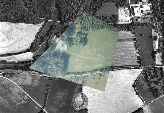
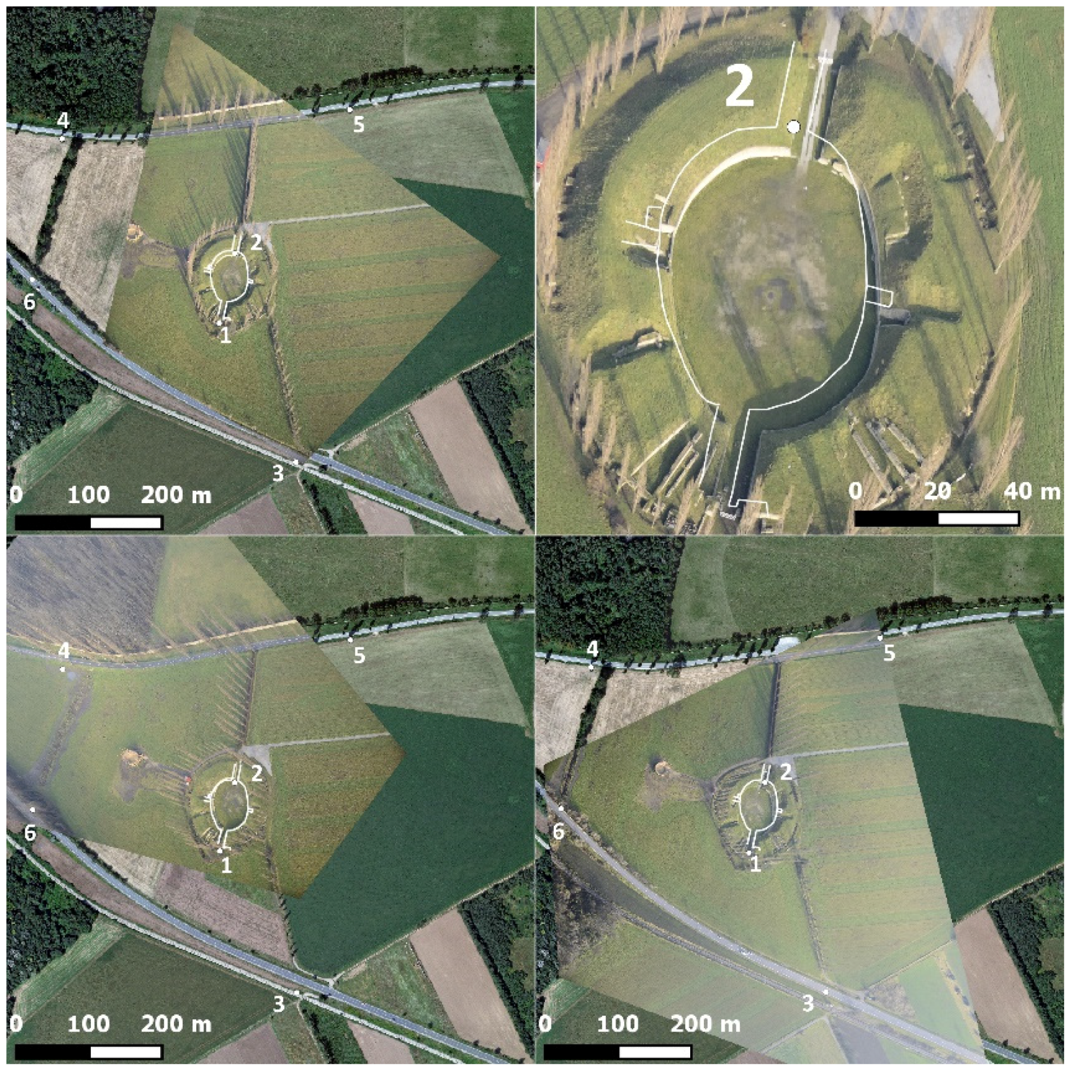
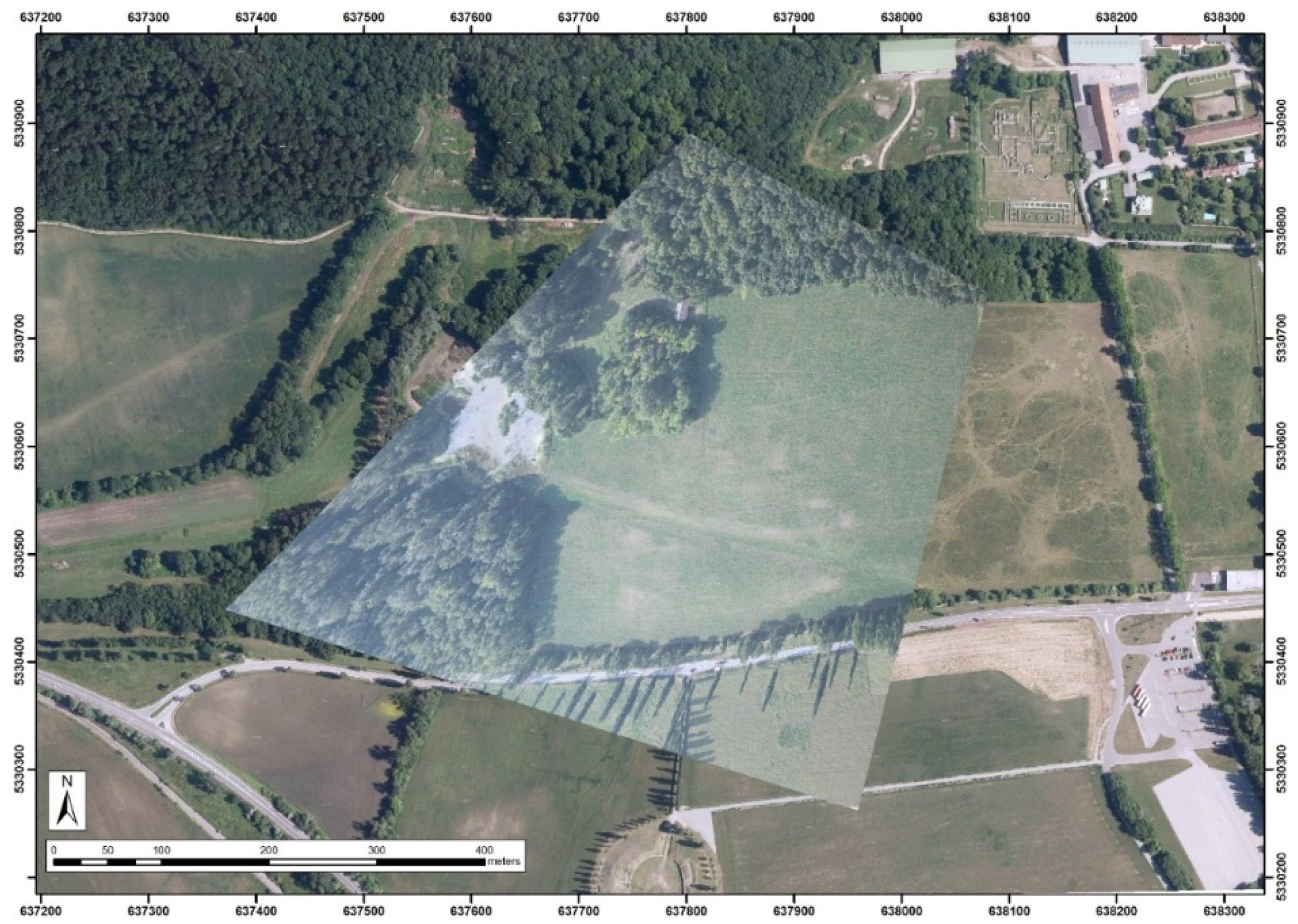
While in the validation section, the accuracy of the angular measurements and the GPS position were investigated, this section also discusses the achieved accuracy in terms of archival needs. The accuracy of the derived footprints turned out to be sufficient for archaeological survey demands. Figure 10 displays the transformation of a low-oblique photograph based on its calculated footprint. While the sides of the trapezoidal footprint measure between min 315 (north) and max 620 m (west), the positional errors of object points lie between 6 m (foreground of photo, i.e., north) and 20 m (background, southern edge). This error lies between only 2% and 3% of the side length.

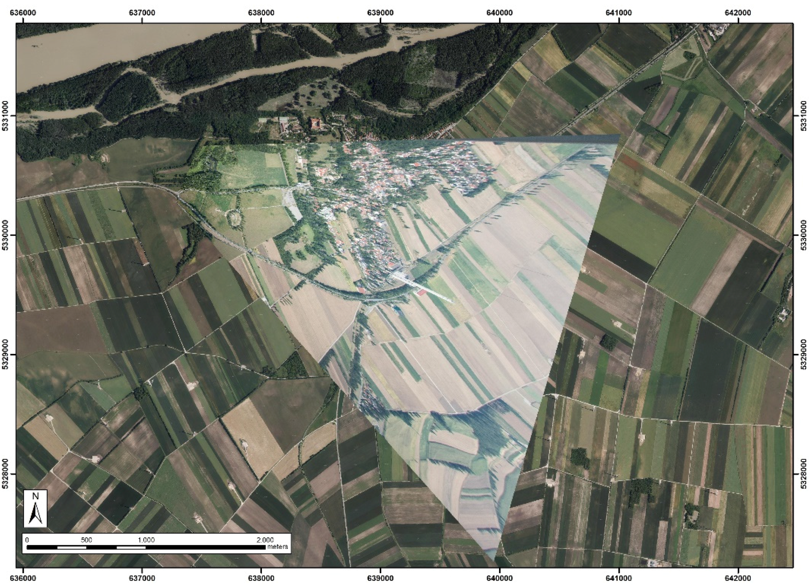
In Figure 11 a high-oblique photograph is monoplotted. Here, the inaccuracies of the positioning of the corners are expected to be far higher in the background than in the low-oblique case of Figure 10. While the sides of the trapezoidal footprint measure between min 512 (west) and max 4000 m (south), the positional errors of object points lie between 26 (foreground of photo, i.e., north) and 400 m (background, southern edge), which corresponds to 5% (foreground) and 10% (background) of the side length. Still in this extreme case, the inaccuracies of the footprint meet our demand stated above in Section 3.

Overall, the results demonstrate that the accuracy and precision of the provided exterior orientation is more than sufficient for automated image archiving of aerial archaeological frame imagery. Throughout all mentioned flight maneuvers, the accuracy stayed within the required limits of 10% of the image width. However, the transformations would not be accurate enough for direct interpretative mapping, since the latter still needs a separate and dedicated orthorectification of the imagery. However, the footprints are used and integrated into our archiving workflow, where they are stored in a data layer within our GIS-based archive (Archaeological Prospection Information System (APIS); see [7]) and as such enable a fast and accurate retrieval of images that cover a specific geographical location.

Moreover, this information can be used in speeding up the orthophoto and DSM creation in a computer vision-based workflow. Since its introduction in archaeological research about fifteen years ago (e.g., [18,19]), the computer vision techniques known as SfM and dense multi-view stereo (MVS) became very popular in archaeology. Nowadays, an SfM and MVS pipeline (generally called image-based modelling) can almost be considered a standard tool in many aspects of both aerial and terrestrial archaeological research (e.g., [20,21,22,23,24,25,26,27,28,29,30,31,32,33]). Even though besides the camera pose, also the parameters of inner orientation may be computed during the SfM stage [34,35], the internal camera parameters can be accurately determined beforehand by a geometric camera calibration procedure [36]. This leaves only the exterior parameters to be computed, and the SfM algorithm can benefit from initial values that are provided by the IMU and GNSS log files, which means that processing time and gross relative orientation errors of the photographs can be minimized. This is incorporated into OrientAL [37], a photogrammetric package recently developed with the financial support of the Austrian Science Fund (FWF P24116-N23). Besides the relative image orientation, OrientAL also aims to automate the process of absolute orientation by automatically extracting GCPs from existing datasets (further details can be found in [37]). A validation of our complete OrientAL-based workflow, using the logged camera positions and rotation angles as initial values, will be the topic of a further paper.

7. Conclusions

The paper proposes a new image archiving workflow, which allows one to automatically derive both the center point and image footprint from oblique aerial photographs made using consumer D-SLR cameras. The proposed workflow is based on the parameters that are logged by a commercial, but cost-effective GNSS/IMU solution and processed with in-house-developed software.

The presented solution is based on the Xsens MTi-G-700-GPS/INS providing both geographical coordinates through its GPS receiver and, using a Kalman filter, camera rotation angles by the inertial measurement unit. The GPS/INS was tested with both a Nikon D800 and a D810 camera. Proper and permanently stable IMU mounting is realized by utilizing the external battery grip of the Nikon D800/D810 as a container for the IMU.

The on-the-fly Kalman-filtered GPS/INS data stream (with 200 Hz for the orientation, 50 Hz for the positional information and 4 Hz for the raw GPS stream) is saved on a standard SD memory card. The post-processing software is a custom-built MATLAB-based program. It calculates and stores the exterior orientation of each photograph, computes the location of ground-projected image center and footprint and optionally executes a projective transformation of each image.

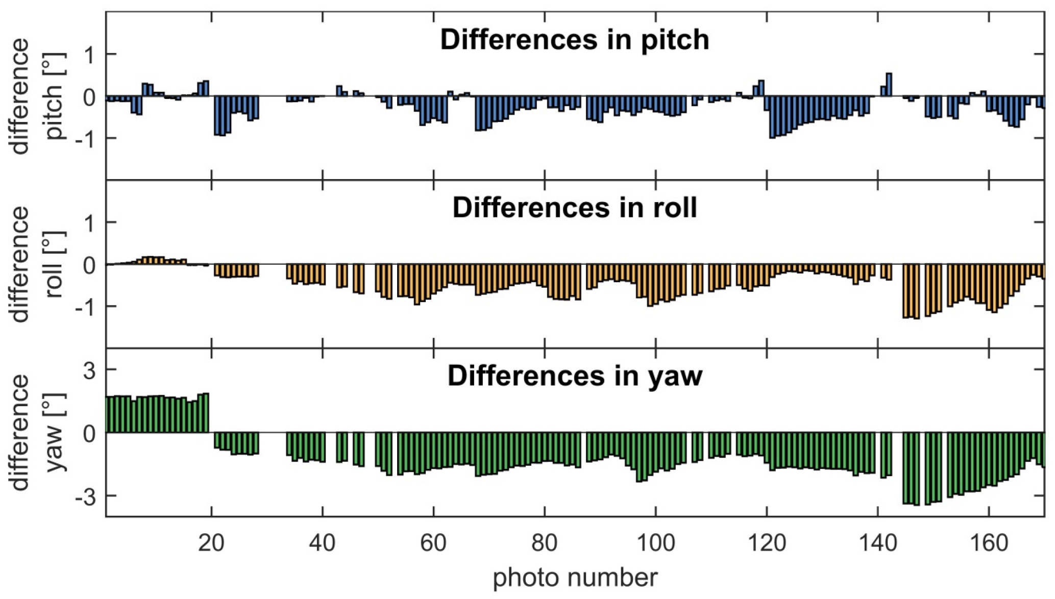
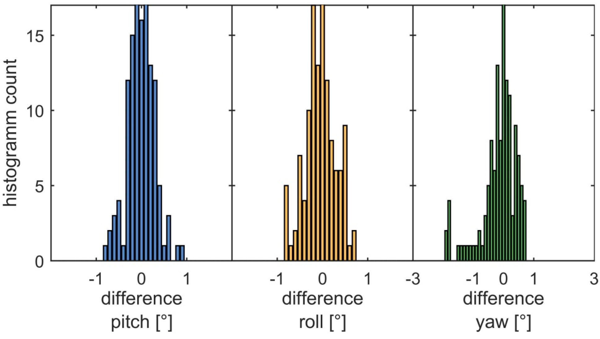
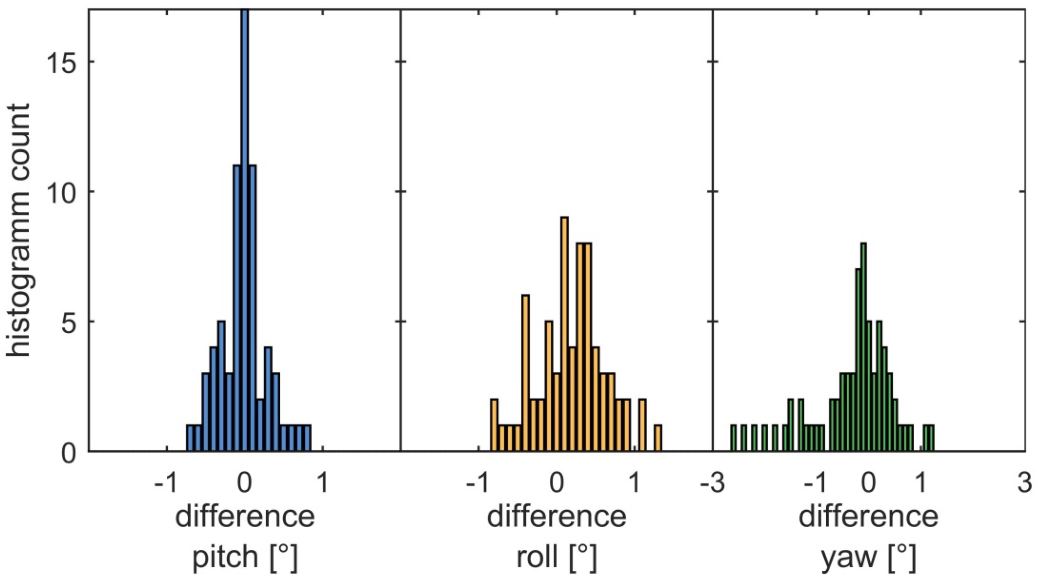
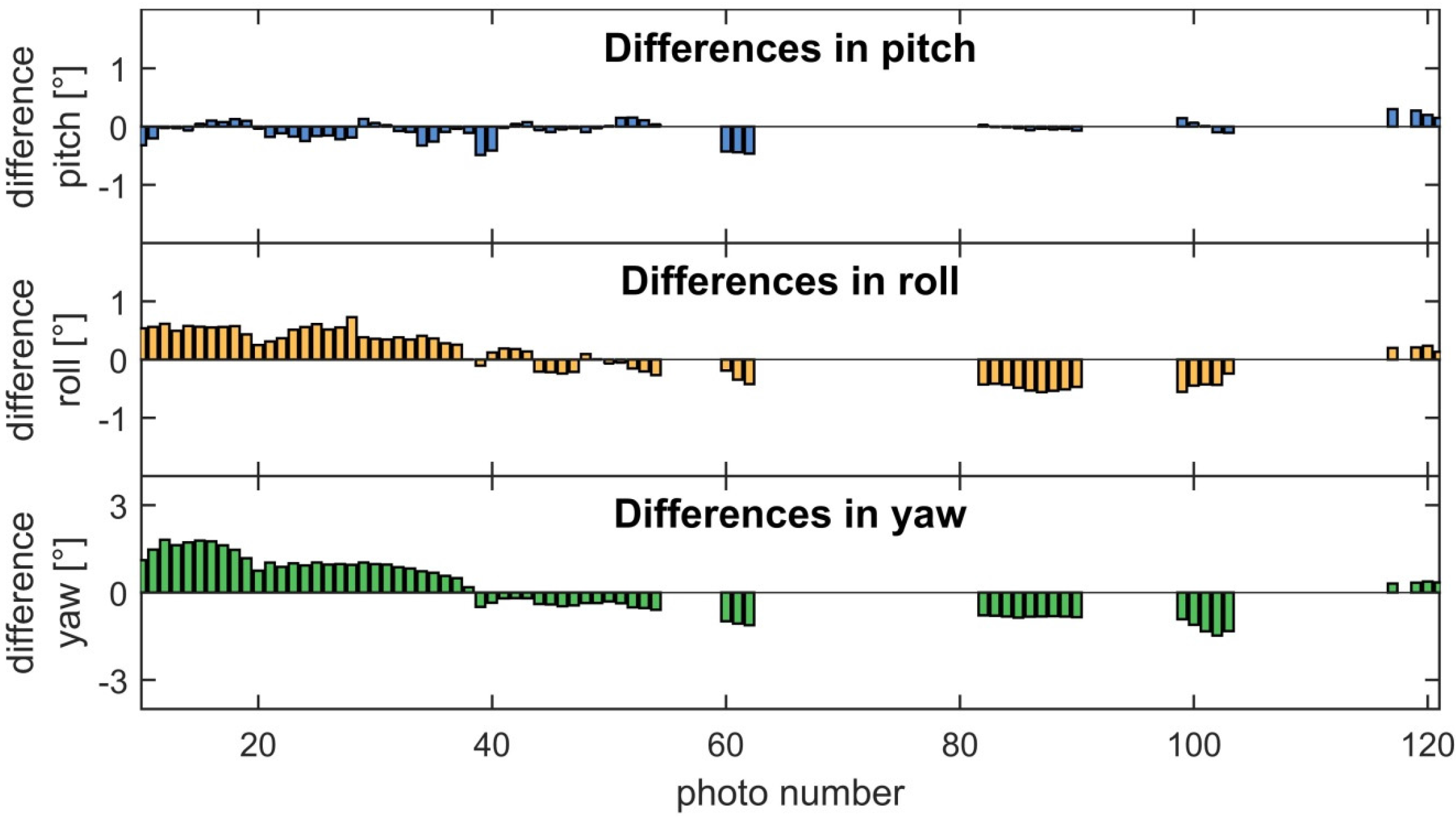
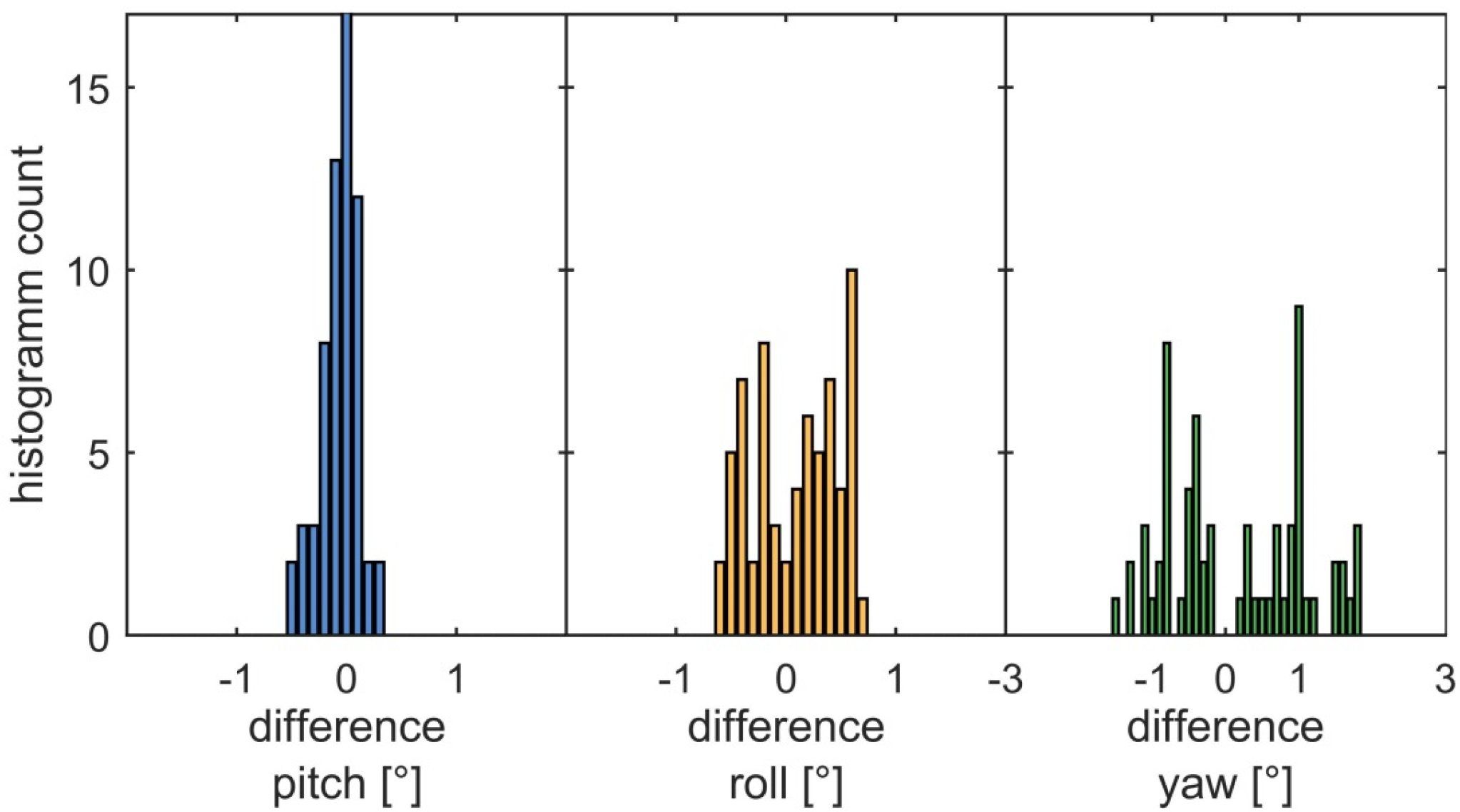
The accuracy and usability of the device was tested within three test flights over pre-defined areas with ground-control targets. First, the exterior orientation values acquired by SfM and the GPS/INS were directly compared and statistically analyzed. The accuracy of the derived angles turned out to be better than 1° for roll and pitch (mean between 0.0 and 0.21 with a standard deviation of 0.17–0.48) and better than 2.5° for yaw angles (mean between 0.0 and −0.14 with a standard deviation of 0.58–0.94). In a second validation step, the locations of the images’ footprint corners were compared to their expected locations derived from an external orthophotograph. In all cases, the deviation was less than 10% of the respective image side length. This seems to be sufficient to enable a fast and almost automatic GIS-based archiving of all of the imagery.

Next to the fact that the presented device enables automated GIS-based archiving of oblique aerial photographs, the derived exterior orientation information can be used in speeding up the orthophoto and DSM creation in a computer vision-based workflow. Although this paper focuses on an archaeological application of the device, the proposed solution can be of interest for all other sciences and applications that are in need of a quick way to directly geolocate aerial and terrestrial photographs.

References

1. Wilson, D.R. Air Photo Interpretation for Archaeologists, 2nd ed.; Tempus: Stroud, Gloucestershire, UK, 2000. [Google Scholar]
2. Verhoeven, G.J.J.; Wieser, M.; Briese, C.; Doneus, M. Positioning in time and space:Cost-effective exterior orientation for airborne archaeological photographs. ISPRS Ann. Photogramm. Remote Sens. Spatial Inf. Sci. 2013, II-5/W1, 313–318. [Google Scholar] [CrossRef]
3. Wieser, M.; Verhoeven, G.J.J.; Briese, C.; Doneus, M.; Karel, W.; Pfeifer, N. Cost-effective geocoding with exterior orientation for airborne and terrestrial archaeological photography: Possibilities and limitations. Int. J. Herit. Digit. Era 2014, 3, 97–121. [Google Scholar] [CrossRef]
4. Doneus, M.; Neubauer, W. Archäologische Prospektion in Österreich. Archäol. Österreichs 1997, 8, 19–33. [Google Scholar]
5. Doneus, M.; Scollar, I. Using GPS with Digital Cameras. AARGnews 2006, 33, 28–33. [Google Scholar]
6. Schmidt, A. Remote Sensing and Geophysical Prospection. Interent Archaeol. 2004, 15. [Google Scholar] [CrossRef]
7. Doneus, M.; Fornwagner, U.; Kiedl, C. APIS—Archaeological Prospection Information System. In Proceedings of the 10th International Conference on Archaeological Prospection, Vienna, Austria, 29 May–2 June 2013; Neubauer, W., Trinks, I., Salisbury, R.B., Einwögerer, C., Eds.; Austrian Academy of Sciences: Vienna, Austria, 2013; pp. 317–318. [Google Scholar]
8. Verhoeven, G.J.J.; Sevara, C.; Karel, W.; Ressl, C.; Doneus, M.; Briese, C. Undistorting the past: New techniques for orthorectification of archaeological aerial frame imagery. In Good Practice in Archaeological Diagnostics: Non-Invasive Survey of Complex Archaeological Sites; Corsi, C., Slapšak, B., Vermeulen, F., Eds.; Springer International Publishing: Cham, Switzerland, 2013; pp. 31–67. [Google Scholar]
9. Mikhail, E.M.; Bethel, J.S.; McGlone, J.C. Introduction to Modern Photogrammetry; Wiley: New York, NY, USA, 2001. [Google Scholar]
10. Kraus, K. Photogrammetry: Geometry from Images and Laser Scans, 2nd ed.; Walter de Gruyter: Berlin, Germany; New York, NY, USA, 2007. [Google Scholar]
11. Wolf, P.R.; Dewitt, B.A. Elements of Photogrammetry with Applications in GIS, 3rd ed.; McGraw-Hill: Boston, MA, USA, 2000. [Google Scholar]
12. Verhoeven, G.J.J. Digitally Cropping the Aerial View. On the Interplay between Focal Length and Sensor Size. Archeol. Aerea. Studi di Aerotopogr. Archeol. 2008, 3, 195–210. [Google Scholar]
13. Hofmann-Wellenhof, B.; Lichtenegger, H.; Wasle, E. GNSS—Global Navigation Satellite Systems: GPS, GLONASS, Galileo & More; Springer: Wien, Austria, 2008. [Google Scholar]
14. Xsens technologies B.V. MTi User Manual: MTi 10-Series and MTi 100-Series; Xsens Technologies B.V.: Enschede, The Netherland, 2015. [Google Scholar]
15. Xsens Technologies B.V. MTi 100-Series—The Most Accurate and Complete MEMS AHRS and GPS/INS. 2015. Available online: https://www.xsens.com/wp-content/uploads/2015/05/MTi-100-series.pdf (accessed on 28 September 2015).
16. Neubauer, W.; Gugl, C.; Scholz, M.; Verhoeven, G.J.J.; Trinks, I.; Löcker, K.; Doneus, M.; Saey, T.; van Meirvenne, M. The discovery of the school of gladiators at Carnuntum, Austria. Antiquity 2014, 88, 173–190. [Google Scholar] [CrossRef]
17. Basemap.at. Available online: http://www.basemap.at (accessed on 26 February 2016).
18. Pollefeys, M.; Koch, R.; Vergauwen, M.; van Gool, L. Automated reconstruction of 3D scenes from sequences of images. ISPRS J. Photogramm. Remote Sens. 2000, 55, 251–267. [Google Scholar] [CrossRef]
19. Pollefeys, M.; Koch, R.; Vergauwen, M.; van Gool, L. Virtualizing Archaeological Sites. In Proceedings of the 4th International Conference on Virtual Systems and Multimedia (VSMM) 98, Gifu, Japan, 18–20 November 1998.
20. Remondino, F.; Barazzetti, L.; Nex, F.; Scaioni, M.; Sarazzi, D. UAV photogrammetry for mapping and 3D modeling—Current status and future perspectives. In Proceedings of the International Conference on Unmanned Aerial Vehicle in Geomatics (UAV-g), Zurich, Switzerland, 14–16 September 2011.
21. Reinhard, J. Things on strings and complex computer algorithms: Kite Aerial Photography and Structure from Motion Photogrammetry at the Tulul adh-Dhahab, Jordan. AARGnews 2012, 45, 37–41. [Google Scholar]
22. Lo Brutto, M.; Borruso, A.; D’Argenio, A. UAV Systems for Photogrammetric Data Acquisition of Archaeological Sites. Int. J. Herit. Digit. Era 2012, 1, 7–14. [Google Scholar] [CrossRef] [Green Version]
23. Scollar, I.; Giradeau-Montaut, D. Georeferenced Orthophotos and DTMs from Multiple Oblique Images. AARGnews 2012, 44, 12–17. [Google Scholar]
24. Verhoeven, G.J.J.; Doneus, M.; Briese, C.; Vermeulen, F. Mapping by matching: A computer vision-based approach to fast and accurate georeferencing of archaeological aerial photographs. J. Archaeol. Sci. 2012, 39, 2060–2070. [Google Scholar] [CrossRef]
25. Verhoeven, G.J.J.; Taelman, D.; Vermeulen, F. Computer vision-based orthophoto mapping of complex archaeological sites: the ancient quarry of Pitaranha (Portugal-Spain). Archaeometry 2012, 54, 1114–1129. [Google Scholar] [CrossRef]
26. Verhoeven, G.J.J. Taking computer vision aloft—Archaeological three-dimensional reconstructions from aerial photographs with PhotoScan. Archaeol. Prospect. 2011, 18, 67–73. [Google Scholar] [CrossRef]
27. Kersten, T.P.; Lindstaedt, M. Potential of Automatic 3D Object Reconstruction from Multiple Images for Applications in Architecture, Cultural Heritage and Archaeology. Int. J. Herit. Digit. Era 2012, 1, 399–420. [Google Scholar] [CrossRef]
28. Forte, M.; Dell’unto, N.; Issavi, J.; Onsurez, L.; Lercari, N. 3D Archaeology at Çatalhöyük. Int. J. Herit. Digit. Era 2012, 1, 352–378. [Google Scholar] [CrossRef]
29. Bezzi, L. 3D Documentation of Small Archaeological Finds. 2012. Available online: http://arc-team-open-research.blogspot.com.br/2012/08/3d-documentation-of-small.html (accessed on 11 October 2012).
30. Lerma, J.L.; Navarro, S.; Cabrelles, M.; Seguí, A.E.; Haddad, N.; Akasheh, T. Integration of Laser Scanning and Imagery for Photorealistic 3D Architectural Documentation. In Laser Scanning, Theory and Applications; Wang, C.-C., Ed.; InTech: Rijeka, Croatia, 2011; pp. 413–430. [Google Scholar]
31. Doneus, M.; Verhoeven, G.J.J.; Fera, M.; Briese, C.; Kucera, M.; Neubauer, W. From deposit to point cloud—A study of low-cost computer vision approaches for the straightforward documentation of archaeological excavations. Geoinformatics 2011, 6, 81–88. [Google Scholar] [CrossRef]
32. Opitz, R.S.; Nowlin, J. Photogrammetric Modeling + GIS: Better Methods for Working with Mesh Data. Available online: http://www.esri.com/news/arcuser/0312/files/archaeology-inventory.pdf (accessed on 8 January 2016).
33. Lo Brutto, M.; Meli, P. Computer Vision Tools for 3D Modelling in Archaeology. Int. J. Herit. Digit. Era 2012, 1, 1–6. [Google Scholar] [CrossRef] [Green Version]
34. Szeliski, R. Computer Vision: Algorithms and Applications; Springer: New York, NY, USA, 2011. [Google Scholar]
35. Hartley, R.; Zisserman, A. Multiple View Geometry in Computer Vision, 2nd ed.; Cambridge University Press: Cambridge, UK, 2003. [Google Scholar]
36. Sewell, E.D.; Livingston, R.G.; Quick, J.R.; Norton, C.L.; Case, J.B.; Sanders, R.G.; Goldhammer, J.S.; Aschenbrenner, B. Aerial cameras. In Manual of Photogrammetry, 3rd ed.; Thompson, M.M., Eller, R.C., Radlinski, W.A., Speert, J.L., Eds.; American Society of Photogrammetry: Falls Church, VA, USA, 1966; pp. 133–194. [Google Scholar]
37. Karel, W.; Doneus, M.; Verhoeven, G.J.J.; Briese, C.; Ressl, C.; Pfeifer, N. OrientAL—Automatic geo-referencing and ortho-rectification of archaeological aerial photographs. ISPRS Ann. Photogramm. Remote Sens. Spatial Inf. Sci. 2013, II-5/W1, 175–180. [Google Scholar] [CrossRef]
Figure 1. The interior orientation of a camera (illustration by M. Doneus).
Remotesensing 08 00209 g001
Figure 2. The exterior orientation of a photograph in relation to a global coordinate reference system (CRS) (X, Y, Z) (illustration by G. Verhoeven).
Remotesensing 08 00209 g002
Figure 3. A Nikon D810 with the detached battery grip, which houses the GPS/INS and logging hardware. The GNSS antenna (square device in the upper right area) is connected with a 2 m-long cable with the logging hardware. The spiral flash sync cord connects the camera and logging hardware (photo: G. Gattinger).
Remotesensing 08 00209 g003
Figure 4. The differences between the indirect (SfM-computed) angles and those from the GPS/INS for the photographs of Flight 1.
Remotesensing 08 00209 g004
Figure 5. Histogram of differences between the indirect (SfM-computed) angles and those from the GPS/INS for Flight 1 after mounting calibration. The first images acquired during the initial state of INS are dismissed.
Remotesensing 08 00209 g005
Figure 6. Orthophotograph that covers the civil amphitheater in Carnuntum, which is used to validate the positional accuracy of the monoplotted images (using the indicated outlines and Points 1–6). Background orthophotograph: © County of Lower Austria, 2008.
Remotesensing 08 00209 g006
Figure 7. (upper left) image 1 (46mm focal length; 44.9° pitch; 7.1° roll and 69.1° yaw); (upper right) zoom of image 1; (lower left) image 2 (50 mm focal length; 31.19° pitch; 4.21° roll and 162.68° yaw); (lower right) image 3 (32 mm focal length; 32.5° pitch; 3.1° roll and −135.8° yaw).
Remotesensing 08 00209 g007
Figure 8. Distances of mapped points to reference positions in the orthophotograph real positions; (left) ordered by photo number; (right) ordered by pitch angle.
Remotesensing 08 00209 g008
Figure 9. Area of Carnuntum, Lower Austria. White line: recorded flightpath of the aerial archaeological reconnaissance flight from 11 August 2015. Red quadrangles: calculated footprints from all photographs, which were taken during the flight over the area of Carnuntum. Background data source: basemap.at [17].
Remotesensing 08 00209 g009
Figure 10. Carnuntum, Lower Austria. Transformation of a low-oblique photograph (pitch = 33°) based on its calculated footprint. Background data source: basemap.at [17].
Remotesensing 08 00209 g010
Figure 11. Carnuntum, Lower Austria. Transformation of a rather high-oblique photograph (pitch = 24°, but no horizon visible) based on its calculated footprint. Background data source: basemap.at [17].
Remotesensing 08 00209 g011