Estimating Evapotranspiration of an Apple Orchard Using a Remote Sensing-Based Soil Water Balance

Abstract

The main goal of this research was to estimate the actual evapotranspiration (ET_c) of a drip-irrigated apple orchard located in the semi-arid region of Talca Valley (Chile) using a remote sensing-based soil water balance model. The methodology to estimate ET_c is a modified version of the Food and Agriculture Organization of the United Nations (FAO) dual crop coefficient approach, in which the basal crop coefficient (K_cb) was derived from the soil adjusted vegetation index (SAVI) calculated from satellite images and incorporated into a daily soil water balance in the root zone. A linear relationship between the K_cb and SAVI was developed for the apple orchard K_cb = 1.82·SAVI − 0.07 (R² = 0.95). The methodology was applied during two growing seasons (2010–2011 and 2012–2013), and ET_c was evaluated using latent heat fluxes (LE) from an eddy covariance system. The results indicate that the remote sensing-based soil water balance estimated ET_c reasonably well over two growing seasons. The root mean square error (RMSE) between the measured and simulated ET_c values during 2010–2011 and 2012–2013 were, respectively, 0.78 and 0.74 mm·day⁻¹, which mean a relative error of 25%. The index of agreement (d) values were, respectively, 0.73 and 0.90. In addition, the weekly ET_c showed better agreement. The proposed methodology could be considered as a useful tool for scheduling irrigation and driving the estimation of water requirements over large areas for apple orchards.

1. Introduction

The Maule region is the most important producer of apples (Malus domestic Mill.) in Chile, with 18,863 ha that represent 63% of the national cultivated surface [1]. During the growing season, rainfall amounts do not cover crop evapotranspiration requirements, so all fruit orchards need to be irrigated. In recent years, water storage has decreased steadily due to the increase in irrigated surfaces, and the droughts caused by El Niño and the Southern Oscillation ENSO climatic phenomena [2].

Consequently, a better understanding of the soil water balance and factors that control crop evapotranspiration (ET_c) are critical for saving water and for proper irrigation management. An operational and accepted method to estimate crop water requirements is the well-known “two step” methodology that combines the reference evapotranspiration (ET_o) and crop coefficients (K_c) [3,4]. Evapotranspiration is estimated by means of single or dual crop coefficient approaches as described in the FAO-56 model approach. A dual crop coefficient distinguishes the effect of crop transpiration and soil evaporation separately [5]. The dual approach seems to be the most convenient to calculate ET_c in apple orchards, because, in general, fruit orchards have a significant area of bare soil in between the rows of trees, which means that the soil evaporation could be an important parameter in the estimation of ET_c. The “two step” methodology can be used in real time irrigation scheduling, but its accuracy is strongly based on adequate knowledge of the K_c values.

In the past three decades, several methods have been developed to experimentally estimate ET_c and K_c (e.g., Bowen ratio, eddy covariance systems, weighing lysimeters), but they are usually expensive and difficult to implement and maintain. Moreover, the use of generic or tabulated K_c values requires knowledge of the crop growth stages, specifically the date when the effective cover occurs, which is affected by management and plant characteristics (size, shape, orientation and distribution of leaves) and the development of the root system [6]. Most of the crop coefficients depend on climate, crop variety, management practices, soil type, irrigation method, and canopy architecture [3,7,8,9,10], and, therefore, a specific adjustment of crop coefficients is required [11]. Particularly for apple orchards, values of crop coefficients depend on the intercepted radiation and may vary with different orchard conditions (row and tree spacing, tree age and size, training system, row orientation) [12]. In addition, most apple varieties have self-incompatibility. Thus, growers usually include more than one variety within each plot [13].

In parallel, since the beginning of the eighties, several studies have shown the utility of remote sensing to derive the basal crop coefficient related to plant transpiration (K_cb) from reflected canopy radiation through vegetation indices (VI) [14]. K_cb can be related to VI because both are sensitive to fractional ground cover and leaf area index [15,16,17,18,19]. Thus, K_cb derived from VI allows the calculation of ET_c and the assimilation of remote sensing data into the soil water balance based on the FAO-56 dual method (VI-ET_o approach) for irrigation scheduling, as well as an extension of the estimation of the crop coefficient from plot scale to field or regional scale [8,20,21,22,23,24,25,26,27]. VI calculated from multispectral satellite images allows for the estimation of the crop evapotranspiration at a pixel scale, where each pixel represents a unique vegetation-soil system [28]. The VI-ET_o approach is suitable even when using imagery from satellites with low revisit frequency, when interpolation is necessary. Interpolated VI are subject to less uncertainty than interpolated ET_c, especially with low vegetation cover and a wet soil surface which generates large ET_c fluctuations [27].

The VI-ET_o approach has been applied and validated for the estimation of ET_c and the assessment of irrigation extensively in herbaceous crops, and slightly in row structured fruit trees (mostly in grapes) [8,20,27,29,30]. However, very few studies have addressed the estimation of crop coefficients, ET_c [31] and irrigation requirements from remote sensing data for apple tree orchards at field scale.

In this context, the main objective of this study is to determine the evapotranspiration and irrigation requirements of a drip-irrigated apple orchard using a one-layer satellite-based soil water balance model by incorporating satellite reflectance data into the soil water balance through the use of the K_cbVI relationship.

2. Materials and Methods

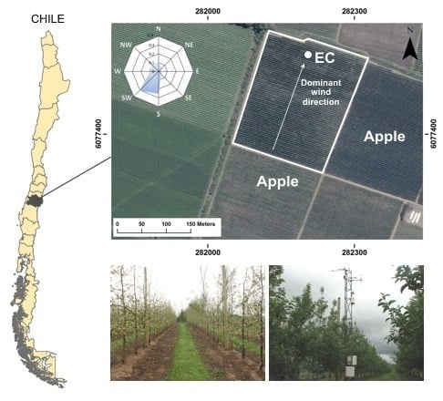
2.1. Site Description

The study was carried out in a drip-irrigated apple (Malus domestica Mill., cv. Pink lady) orchard located in the Talca Valley, Maule Region, Chile (35°25′17″S; 71°23′57″W, 197 m above sea level) during the 2010–2011 and 2012–2013 growing seasons (Figure 1). The climate of the area is described as Mediterranean semi-arid (Csb) according to the Köppen–Threwartha climate classification system [10], with 676 mm of annual rainfall, mostly concentrated in the fall and winter. The average mean, maximum and minimum annual temperatures are 14.3, 21.7 and 8.1 °C, respectively. The soil is classified as Ultic Haploxeralfs (Alfisol) with a clay loam texture at the surface and a clay texture at depth [32], according to the System of Soil Classification of the United States Department of Agriculture [33].

The experimental plot was a 5.2 ha commercial block planted in 2008 with “Pink lady” apple trees on M7 rootstock. Apple trees were in a high density planting system (1.5 × 4 m spacing) and trained on the solaxe system, bending the fruiting branches artificially or naturally and developing free growing fruiting branches [34]. The irrigation system was a surface drip with 4 emitters per tree (4 L·h⁻¹ per emitter). There were double pipelines per tree row, one on each side of the trunk. The emitters along the lines were spaced at 0.75 m. The volumetric soil water content at field capacity was 0.38 m³·m⁻³ (or 304 mm), and the wilting point was 0.25 m³·m⁻³ (or 200 mm) for the effective rooting depth (0.8 m).

The tree rows were orientated in the East-West direction, and the average tree height was between 3.5–4 m. Fruit thinning was carried out every season to obtain a crop load between 200–250 fruits per tree. Apple orchard management was oriented toward increasing the yield, fruit size and fruit quality. The soil surface was covered by growing weeds from the initial growth stage to December.

2.2. Soil Water Balance Driven by Remote Sensing Data

In this study, a remote sensing-based soil water balance performed in the root zone was applied to estimate actual evapotranspiration. The soil water balance was expressed in terms of root zone water depletion following FAO-56 approach [3]:

$${\mathrm{D}}_{\mathrm{r},\mathrm{i}}={\mathrm{D}}_{\mathrm{r},\mathrm{i}-1}-{\mathrm{P}}_{\mathrm{i}}-{\mathrm{I}}_{\mathrm{i}}+{\mathrm{ET}}_{\mathrm{c}}+{\mathrm{DP}}_{\mathrm{i}}$$

(1)

where P_i is precipitation (mm), I_i is irrigation (mm), ET_c is actual evapotranspiration (mm) and DP_i is deep percolation (mm). D_r,i and D_r,i−1 are the cumulative depletion depths (mm) at the end of days i and i−1. An initial depletion D_r,i−1 of zero was assumed—following a heavy rain to initiate the water balance. This value correspond to the D_r,i at the beginning of the next day, thus the depletion at the end of the day D_r,i is recalculated after any drainage loss is estimated and after any reduction in ET_c, to account for low soil water content. Based on the behavior of the ground water level and intensity of rainfall at the study site, the water balance equation was simplified by neglecting capillary rise and surface water run-off. Soil water content sensors buried at different depths showed that capillary rise did not occur into the root zone, whereas run-off was neglected for two reasons: first, the gentle slopes in the field, and second, rainfall usually does not occur during the irrigation season. The water balance methodology allowed an assessment of the comparison between simulated and observed values, and its formulation can also be inverted to estimate irrigation requirements.

The evapotranspiration was calculated following the FAO-56 dual crop coefficient approach, described in depth by [3]. We will present a brief description of the dual crop coefficient methodology and further modifications for the assimilation of remote sensing data. In the dual crop coefficient approach, ET_c is estimated as follows [3]:

$${\mathrm{ET}}_{\mathrm{c}}=\left({\mathrm{K}}_{\mathrm{s}}{\mathrm{K}}_{\mathrm{cb}}+{\mathrm{K}}_{\mathrm{e}}\right){\mathrm{ET}}_{\mathrm{o}}$$

(2)

where K_cb is the transpiration coefficient or basal coefficient, K_e is the evaporation coefficient of the bare soil fraction and K_s is the water stress coefficient. The equations to derive these three coefficients are described below.

2.2.1. Calculation of Satellite-Based Basal Crop Coefficient

The basal crop coefficient (K_cb) represents primarily the transpiration component of ET_c including a small evaporation component supplied by soil water below the dry surface and by soil water from beneath dense vegetation [3,7]. Values of K_cb reported in the literature for many crops have been obtained for specific conditions and can differ considerably from local conditions. As mentioned previously in the introduction, remote sensing is a useful tool to obtain an actual reflectance-based crop coefficient. In this work, K_cb values of a drip-irrigated apple orchard were obtained using a linear regression between the measured basal crop coefficient and the soil adjusted vegetation index (SAVI) obtained from canopy reflectance using satellite images [8,15,19,26]. Measured values of the ground K_cb were obtained using the ratio of ET_c from an eddy covariance system to grass reference evapotranspiration (ET_o) selecting dates with no stress and minimum soil evaporation (3–4 days following an irrigation or rain event).

2.2.2. Calculation of Soil Evaporation Coefficient

The soil evaporation coefficient (K_e) was estimated based on the daily calculation of the water balance in the topsoil evaporation layer as is stated in FAO-56 [3]:

$${\mathrm{K}}_{\mathrm{e}}={\mathrm{K}}_{\mathrm{r}}\left({\mathrm{K}}_{\mathrm{c}\_\max }-{\mathrm{K}}_{\mathrm{cb}}\right)\le \left(1-{\mathrm{f}}_{\mathrm{c}}\right){\mathrm{K}}_{{\mathrm{c}}_{\max }}$$

(3)

where K_r is a soil evaporation reduction coefficient, K_{c_max} is the maximum value of crop coefficient and f_c is the fraction cover. The maximum value of the crop coefficient was set equal to 1.2 because of the contribution of evaporation from wetting intervals greater than 3 or 4 days [3], and the fraction cover values were derived from SAVI values using the relationship obtained by [35] for a row structured vineyard.

Some authors have shown that under high evaporation conditions, the FAO-56 model overestimates soil evaporation at the beginning of the process [36,37]. We applied the correction proposed by [37] to improve the daily evaporation estimation of FAO-56 using the reduction of the readily evaporable water (REW) coefficient to limit stage I (evaporation occurs at the same rate as atmospheric demand) and the application of a factor (m) to reduce the K_r coefficient in stage II (evaporation is lower than the atmospheric demand as a consequence of soil retention forces). In this study, a reduction factor of 0.5 was adopted. Considering the correction, values of K_r can be computed as:

$${\mathrm{K}}_{\mathrm{r}}=\min \left\{\frac{\mathrm{REW}}{\mathrm{ETo}},\mathrm{m}\frac{\mathrm{TEW}-{\mathrm{D}}_{\mathrm{e},\mathrm{i}}}{\mathrm{TEW}-\mathrm{REW}}\right\}$$

(4)

where the REW was set equal to 4 mm according to the model calibration proposed by [37]. The cumulative water depletion at the end of day i in the evaporable layer (D_e,i) was obtained by computing a daily soil water balance in the surface soil evaporation layer. The total evaporable water (TEW) was estimated as TEW = (θ_FC − 0.5 θ_WP)∙Z_e, where Z_e is the depth of the soil surface evaporation layer (m).

2.2.3. Estimation of Water Stress Coefficient

In a similar way to the K_e coefficient, the estimation of the water stress factor (K_s) involves the computation of a daily soil water balance in the root zone. The estimation of K_s requires the definition of a threshold value of the mean water content at the root zone, expressed as the cumulative water depletion depth for day i (D_r,i). Water stress begins when D_r,i exceeds the readily available water in the root zone (RAW). For D_r,i < RAW, K_s = 1, whereas for D_r,i > RAW, K_s is calculated as:

$${\mathrm{K}}_{\mathrm{s}}=\frac{\mathrm{TAW}-{\mathrm{D}}_{\mathrm{r},\mathrm{i}}}{\mathrm{TAW}-\mathrm{RAW}}=\frac{\mathrm{TAW}-{\mathrm{D}}_{\mathrm{r},\mathrm{i}}}{\left(1-\mathsf{\rho }\right)-\mathrm{TAW}}$$

(5)

where TAW (mm) is the total available water in the root zone and ρ is the fraction of TAW that can be depleted from the root zone under non-stress conditions. TAW is estimated as:

$$\mathrm{TAW}=1000\left({\mathsf{\theta }}_{\mathrm{FC}}-{\mathsf{\theta }}_{\mathrm{WP}}\right){\mathrm{Z}}_{\mathrm{r}}$$

(6)

where θ_FC and θ_WP (cm³·cm⁻³) are the soil water content at field capacity and wilting point, respectively, and Z_r is the crop rooting depth (m).

2.3. Soil Water Balance Parameterization

The relationship between the Soil Adjusted Vegetation Index (SAVI) and K_cb allowed the direct integration of VI into the FAO-56 soil water balance model. The spatial representation of the model depends on the scale of the inputs parameters. Working with Landsat images the spatial scale is 30 × 30 m, but, considering the possible inaccuracies in the images processing, we selected a square of 90 × 90 m formed by 9 pixels (around 1 ha). The estimation of K_e was implemented for the apple orchard characteristics, taking into account that the vegetation cover at midseason was 30% and 40% for the 2010–2011 and 2012–2013 growing seasons, respectively. This could lead to a high water evaporation rate after irrigation or rainfall events. According to [37], a value of REW of 4 mm was used to avoid the total consumption of evaporable water in just a few days. A surface soil evaporation layer with a depth of 0.10 m was adopted because the soil is shaded by trees and covered by weeds. The observed fraction of the soil wetted by irrigation events was 0.3, while the fraction of wetted and exposed soil was estimated following the FAO-56 approach. The depletion fraction (p) was set at 0.50 for ET_c, approximately 5 mm·day⁻¹. The field capacity and wilting point were obtained from the soil textures using the equation derived by [38]. The parameters used in this study are shown in

Table 1. Parameters used in the soil water balance based on the FAO-56 methodology for apple orchards.

Parameter	Description	Value
REW (mm)	Readily evaporable water	4
TEW (mm)	Total evaporable water	12.75
Ze (m)	Depth of surface soil evaporation layer	0.10
fw	Fraction of the surface wetted	0.3
θfc (cm3·cm−3)	Field capacity	0.38
θwp (cm3·cm−3)	Wilting point	0.25
Zr max (m)	Maximum effective root deep	0.80
p	Soil depletion fraction without stress	0.50

.

2.4. Experimental Data: EC Fluxes, Meteorological Data, Soil Moisture and Apple Water Status

An eddy covariance system (EC) was installed in the field for three months, coinciding with the midseason growth stage to measure the latent and sensible heat fluxes. In the 2012–13 season, measurements were extended from November 2012 to April 2013. The EC system consists of an open-path infrared gas analyzer (IRGA) (LI-7500, Licor Inc., Lincoln, NE, USA), to measure the concentrations of water vapor and carbon dioxide in the air, and a 3D sonic anemometer (CSAT3, Campbell Scientific Inc., Logan, UT, USA), to measure wind velocity components and temperature variations. In both seasons, the IRGA fast response was calibrated before the field campaign began. The frequency analysis of wind direction showed that the dominant directions were south and southwest (See Figure 1). The sensors were oriented towards the dominant wind direction and located at a height of 6 m above the ground surface. The source area for the turbulent fluxes (fetch) was calculated following [39]. The analysis of the footprint model showed that the peak footprint location (x_max) was obtained at 15 m and a cumulative normalized contribution to the flux measurement (CNF) of 90% was obtained at 278 m that represents a height to fetch ratio of 1:46. This ratio is less than conventional ratio 1:100 usually considered for studies made over agricultural crop surfaces but consistent with other field observations reporting fetch to height ratios ranging from 1:15 to 1:75 [40,41,42,43].

The measurements were sampled at a frequency of 10 Hz and were recorded into high frequency files in a datalogger CR5000 (Campbell Scientific Inc., Logan, UT, USA). The average values were calculated and recorded every 15 min. Raw sensible and latent heat fluxes were corrected for air density fluctuations, effects of sensor separation, sampling frequency and path-length averaging according to [11,44]. Data were averaged to obtain the daily flux values, including data obtained during the night period. The energy fluxes coming from north, northeast and northwest wind direction were rejected and the gaps were imputed based on the environmental conditions associated with the missing data [45,46] using a multivariate model. The associated climatic variables were net radiation, air temperature, relative humidity, vapor pressure deficit, considering the last one as a major driver of latent heat flux [45]. Missing data during some days was due to problems with the power supply and IRGA signal obstruction on rainy days.

In addition to the EC system, a CNR1 net radiometer (Kipp & Zonen B.V., Delft, The Netherlands) was mounted at 5.35 m above the ground to measure the net radiation (Rn), and eight HFP01 plates (Hukseflux B.V., Delft, The Netherlands) were placed at four spatially representative positions (2 intra-row and 2 inter-row) to capture the lighting and shading patterns that can affect the soil heat flux (G) in heterogeneous covers [17] such as fruit orchards. The plates were buried at a depth of 8 cm and were accompanied by two chrome-constantan thermocouples (TCAV, Campbell Sci. Inc.) at depths of 2 and 4 cm. Additionally, two sets of capacitance probes (EC-5 Decagon Devices, Inc., Pullman, WA, USA) were buried at 8, 20, 40 and 60 cm in depth to supervise the irrigation events and the depletion dynamics (data not shown here). One set was placed close to the drip emitters and the other set at the center of the inter-row area. The volumetric water content was obtained through the standard calibration equation recommended by the manufacturer.

The soil heat flux (G) was calculated following the combined method [47], which considers the heat capacity of the surface soil to correct the heat flux measured by plates. G measurements were averaged, taking into account the vegetation fraction cover at midseason (30%–40%). The soil heat flux and temperature measurements were recorded every 10 s and averaged every 15 min in a datalogger CR3000 (Campbell Scientific Inc., Logan, UT, USA). In this study, the energy imbalance was corrected by Bowen Ratio closure approach [48].

The reference evapotranspiration (ET_o) and precipitation were obtained using meteorological data from an automatic weather station—installed over grass with optimum growth conditions—located one km from the experimental site (35°25′20″S; 71°23′11″W). The daily ET_o was calculated using the FAO-56 Penman–Monteith equation [3].

To evaluate the water status of the apple trees, the midday stem water potential was measured by a pressure chamber (PMS600, PMS Instruments Company, Corvallis, OR, USA). The stem water potential was measured at solar noon on 18 fully expanded leaves located near the bases of the trees. Selected leaves were saved in plastic bags covered with aluminum foil for 2 h before the measurement [49]. The measurements were taken weekly from December to January during the 2010–2011 and from November to March during the 2012–2013 growing season.

2.5. Remote Sensing Data Acquisition and Processing

The assessment of the remote sensing-based soil water balance used satellite images acquired by the Landsat-5 thematic mapper (L5-TM), Landsat-7 enhanced thematic mapper plus with the scan line corrector off (L7-ETM+) and Landsat-8 operational land imager (L8-OLI) sensors (Path-Row 233-085). Fortunately, the plot is located in the gap-free zone for L7-ETM+ images. Thus, the information provided was useful in describing the temporal evolution of the canopy. The images were provided by the NASA Land Processes Distributed Active Archive Center (LPDAAC, Sioux Falls, SD, USA) and selected using the Global Visualization Viewer (GloVis) tool. Twenty-five cloud-free images over the study area were used with a minimum of nine images per growing campaign. The image dates are listed in

Table 2. Sensor and image acquisition date for the apple orchard.

Season 2010–2011		Season 2012–2013
Date	Sensor	Date	Sensor
6 November 2010	L7-ETM+	26 October 2012	L7-ETM+
14 November 2010	L5-TM	11 November 2012	L7-ETM+
30 November 2010	L5-TM	27 November 2012	L7-ETM+
08 December 2010	L7-ETM+	29 December 2012	L7-ETM+
16 December 2010	L5-TM	30 January 2013	L7-ETM+
1 January 2011	L5-TM	15 February 2013	L7-ETM+
9 January 2011	L7-ETM+	3 March 2013	L7-ETM+
25 January 2011	L7-ETM+	19 March 2013	L7-ETM+
2 February 2011	L5-TM	12 April 2013	L8-OLI
26 February 2011	L7-ETM+	6 May 2013	L7-ETM+
22 March 2011	L5-TM	14 May 2013	L8-OLI
30 March 2011	L7-ETM+
23 April 2011	L5-TM
1 May 2011	L7-ETM+

.

Landsat Standard Terrain Correction (Level 1T) data were provided every 16 days. This product has been geometrically corrected and georeferenced. The image processing included the atmospheric and radiometric corrections of the optical bands using the Fast Line-of-sight Atmospheric Analysis of Spectral Hypercubes module (FLAASH) implemented in ENVI 4.5 [50]. The FLAASH code based on the radiative transfer model MODTRAN4 [51] and the 6S model [52] retrieved atmospheric water vapor content and monthly aerosol data. The procedure included the image calibration using the coefficients proposed in the literature for L-5 TM y L-7 ETM+ [53].

To evaluate the performance of the atmospheric correction method, eight surface SAVI images obtained using the FLAASH were compared with SAVI images obtained from Landsat Surface Reflectance products. The comparison was applied to a 3 × 3 km (100 × 100 pixels) section of the study area and did not utilize SAVI values lower than 0.1 (non‑vegetated areas). The values of SAVI obtained by both approaches fit quite well, with a root mean square error (RMSE) lower than 0.00022 for all dates. These results support the atmospheric correction method used in the present study.

In this study, the SAVI was chosen to model the basal crop coefficient [54]. SAVI minimizes the variations in the vegetation index due to the background soil brightness, which could become significant in fruit orchards with heterogeneous cover. SAVI is defined as:

$$\mathrm{SAVI}=\frac{\mathrm{NIR}-\mathrm{red}}{\mathrm{NIR}-\mathrm{red}+\mathrm{L}}\left(1+\mathrm{L}\right)$$

(7)

where NIR and red are the reflectances in the near infrared and red bands of the electromagnetic spectrum, respectively. L is an adjustment factor that reduces the soil background influences under different vegetation cover conditions. The optimal value of L decreases as vegetation cover increases: L = 1 for very low vegetation densities, L = 0.5 for intermediate vegetation densities and L = 0.25 for higher densities. A single value of L = 0.5 was used in this study, which was shown to reduce soil noise considerably throughout the range in vegetation densities [8,20,27,54].

The vegetation indices were calculated on a pixel-by-pixel basis and averaged over a 90 × 90 m area (3 × 3 pixels), departing from the tower station in the main wind direction to represent the heterogeneity in the orchard but avoiding the edge effects.

2.6. Statistical Analysis

Daily and weekly values of measured and estimated ET_c were compared by using a linear regression analysis and a series of statistics described by [55]: RMSE, mean absolute error (MAE), mean bias error (MBE) and index of agreement (d) used as a relative measure of the difference among variables. Perfect agreement would exist between observed and modeled values if d = 1. Additionally, the relative RMSE and relative MAE were provided to evaluate the models performance [56].

3. Results and Discussion

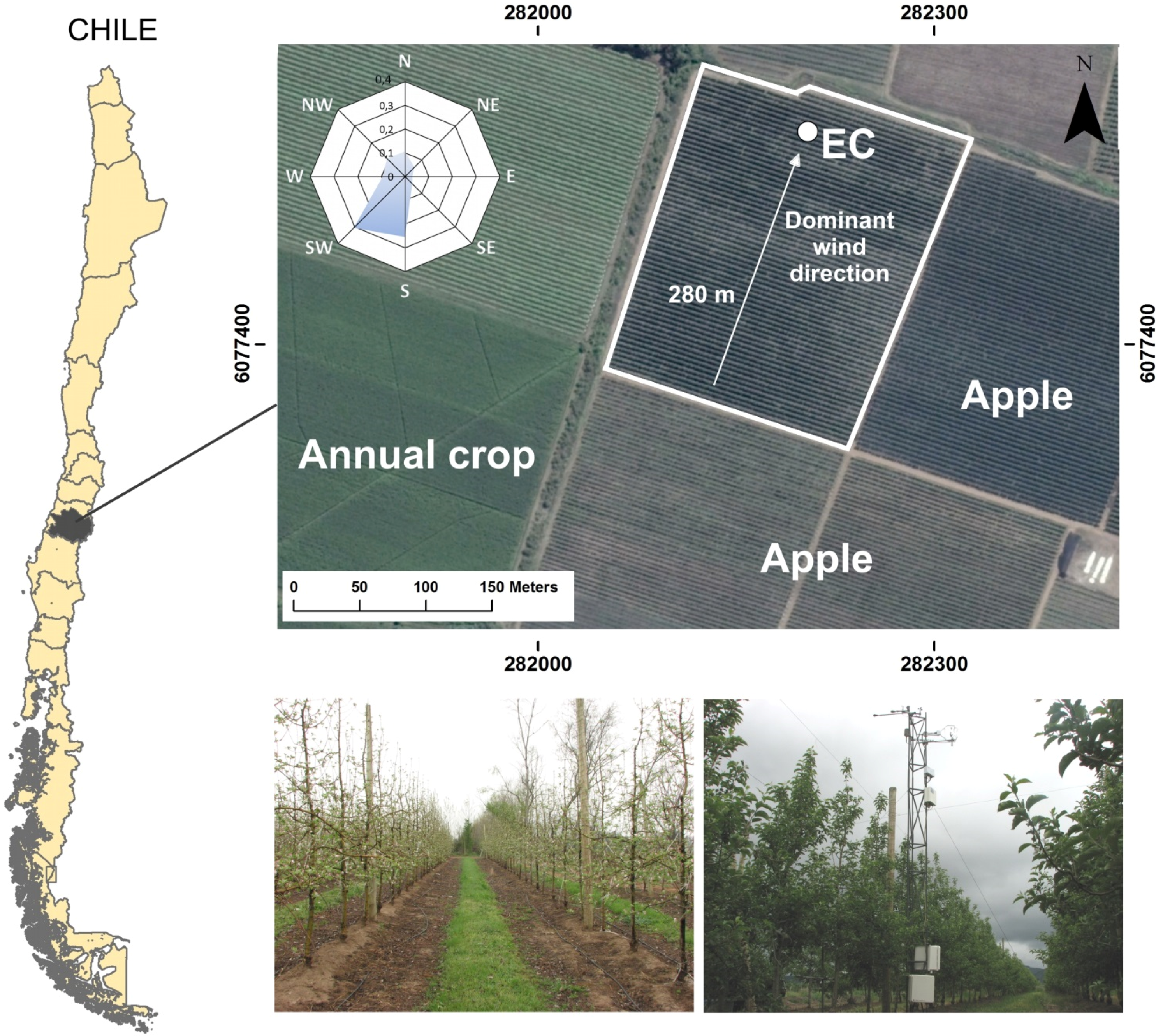
3.1. Meteorological Conditions and Plant Water Status

The temporal evolution of ET_o, the precipitation events and the amount and timing of irrigations applied by the grower for both seasons are shown in Figure 2. The average accumulated values of ET_o were 975 and 875 mm for the 2010–2011 and 2012–2013 growing seasons, respectively. The highest values of ET_o occurred in the summer (6.8 mm during 2010–2011 and 6.6 mm for 2012–2013 season) and the lowest values occurred in the winter (approximately 0.4 mm for both seasons). The total precipitation for the 2010–2011 season was 255 mm, while that for the 2012–2013 season was 373 mm. The irrigation depths applied by the farmer were 547 and 439 mm for the first and second seasons, respectively. The average values of midday stem water potential during the midseason ranged from −0.9 to −1.35 MPa for the 2010–2011 season, while that for the 2012–2013 season ranged from −1.18 to −1.49 MPa, which indicated that the apple trees were not under water stress during most of the growing season, in accordance with previous studies [12,57,58]. The lowest values of midday stem water potential (between −1.65 and −2.01 MPa) were observed during March 2013, indicating that the apple trees could be under moderate water stress on these dates.

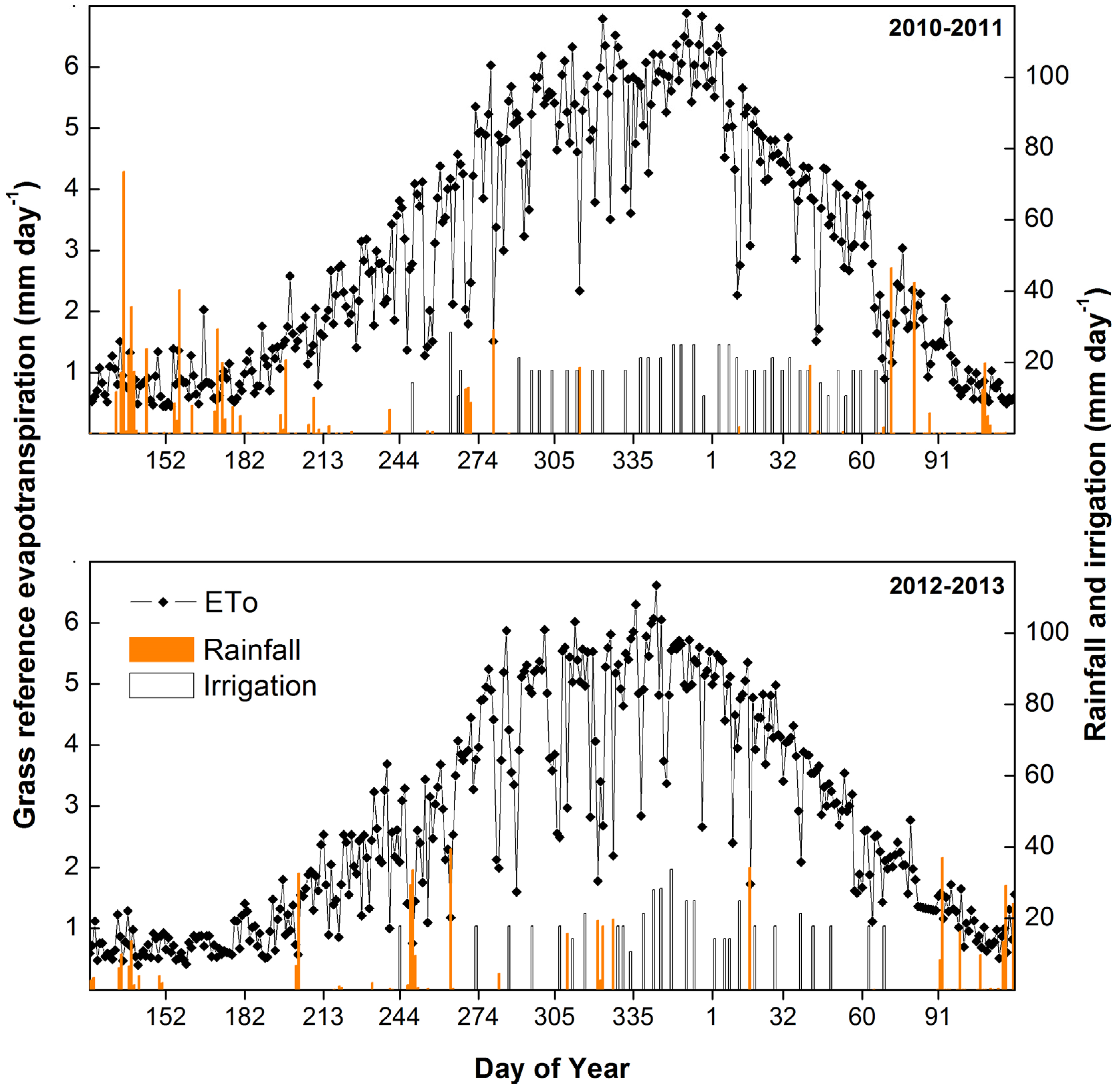
3.2. Energy Balance Closure and Measured Values of ET_c and K_c in the Apple Orchard

Direct measurement of the four energy balance components were evaluated in the analyzed study site. Figure 3 shows the linear fit between the sum of sensible and latent heat fluxes (H + LE) and the available surface energy (Rn − G) at daily time scale. The regression exhibited a slope of 0.87 and an intercept of 13 W·m⁻². The coefficient of determination was 0.83. These results showed an underestimation of the turbulent fluxes lower than 13% of the total available energy and an RMSE of 22 W·m⁻², which is in agreement with other studies based on this type of micrometeorological measurements in similar canopies [59,60]. According with the most recent studies, the lack of energy balance closure does not constitute a clear evidence for erroneous turbulent flux measurements and other causes such the storage of energy and heat in the canopy biomass, the storage of heat in the soil layer over the heat flux sensors and metabolism could contribute to this imbalance [61]. Conversely, many authors propose the correction of energy balance imbalance that could be attributed to measurements errors in Rn and G, inconsistent source areas between EC sensible and latent heat fluxes and surface available energy, length of sampling intervals, sensor separation, and dispersive fluxes not sampled by EC system [62]. The most widespread methods to correct the energy imbalance are the Bowen ratio (BR) and the residual energy correction method (E_R). In this paper we adopted the BR approach suggested by [48] as the most appropriate. The BR correction method assumes that H and LE are underestimated, and available surface energy is considered reliable and representative of the eddy covariance flux footprint. According to [48,63], no compelling evidence exists to confirm that the eddy covariance method only underestimates LE, but BR correction has been effective in other studies over fruit orchards as oranges, olives, vineyards [8,20,42,59,64]. In addition, we founded that the correction of LE flux based on BR method improve the stability of the experimental values of the crop coefficient, reducing the presence of spikes or unreal values in the temporal evolution of this coefficient. The correction based on the BR method increases the LE values in 10 W·m⁻² on average, or 17% of the measured LE data.

The mean daily ET_c measured during the midseason was 3.24 and 3.77 mm for the 2010–2011 and 2012–2013 seasons, respectively, although the ET_c showed a large day-to-day variability (Figure 4). The ET_c values were mainly affected by the daily variation of ET_o, in addition to the effect of irrigation or precipitation events that increased the soil evaporation. On the other hand, the K_c values tended to remain fairly constant during the midseason, although temporal variations were caused by the irrigation frequency (every 3–5 days). The mean value of K_c during the midseason for 2010–2011 season was 0.60, while that for 2012–2013 was 0.77. During both seasons, the maximum K_c values were obtained after irrigation or rainfall events (varying between 0.83 and 1.22), while the minimum K_c values were usually observed 3–4 days after irrigation (between 0.41 and 0.52).

The observed differences between the mean values of K_c for the two studied seasons could be explained by the difference in the peak of the ground cover fraction (30% and 40% in 2010–2011 and 2012–2013 season, respectively). The midseason K_c values obtained in this study were similar to the values reported by [65] (between 0.65 and 0.77) obtained from weighing lysimeter measurements for a Golden Smoothee apple orchard with a comparable canopy size (34%–40%). However, for a cover fraction of 45%, reference [65] observed a higher K_c (1.04). Additionally, references [3,7] suggested K_c values of 1.2 and 1.15, respectively, for apple trees with active ground cover and a fraction cover of 0.5.

The long time series available for the 2012–2013 season allowed the analysis of the temporal evolution of measured K_c values until harvest. From the midseason to harvest, K_c tended to remain constant except after fruit removal, K_c values decreased, reaching minimum values of approximately 0.4. This effect was also reported by [12,65] for Golden Smoothee apples.

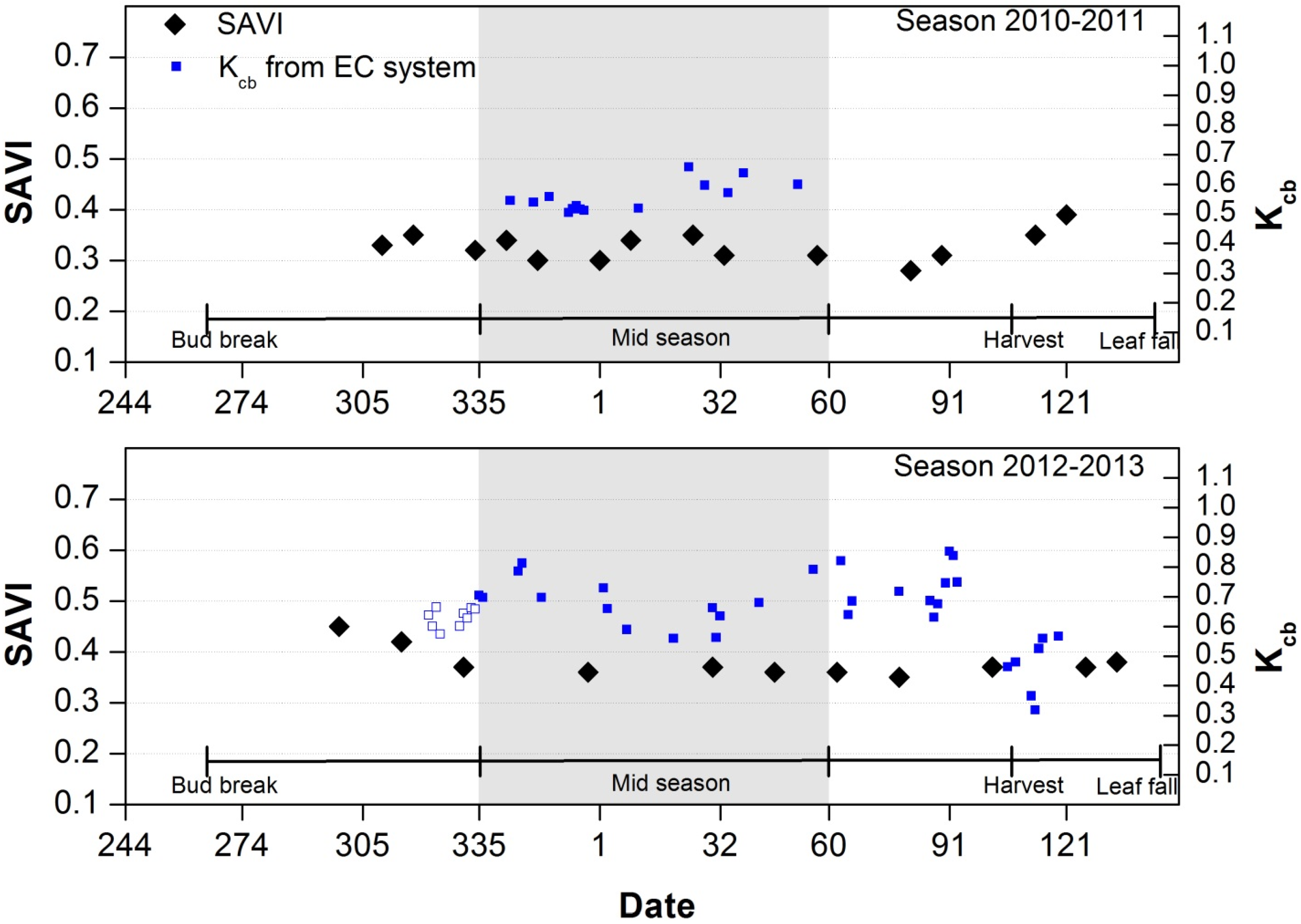
3.3. Seasonal Evolution of SAVI

The seasonal evolution of the SAVI of the drip-irrigated apple orchard is shown in Figure 5 along with the K_cb obtained from eddy covariance system. K_cb and SAVI time series showed to be in agreement. The shaded area represents the midseason, when the inter-row ground cover is dry, and the value of the SAVI were mainly attributable to the apple canopy. However, the SAVI values at the initial, crop development and late season growth stages exhibited the effect of weed cover growing in the inter-row area. It should be noted that the SAVI values at the initial and crop development growth stages represented the growth of the apple-weeds cover mixture. In this study site, the inter row weeds dried naturally in early December for both seasons. From this date until harvest, the SAVI values belonged to the apple canopy. The evolution of SAVI showed the differences of full canopy cover between both growing seasons due to the orchard age. Since the full cover was lower in 2010–2011 season and some precipitation events occurred in March and April, the SAVI values of post-harvest period showed a noted increase due to a greater growth of weeds in early April. The 2012–2013 season showed a constant value of SAVI in post-harvest period until the leaf drop which means a low weeds cover because the precipitation events started in May. However, K_cb values showed a reduction after harvest (Figure 5, 2012–2013 season). Fruit sink removal decreases the tree water use [65]. SAVI was selected to derive K_cb for the apple orchard because it was less sensitive to background effects while NDVI showed a higher variation during the analyzed campaigns that did not correspond with variations in the analyzed canopy [54].

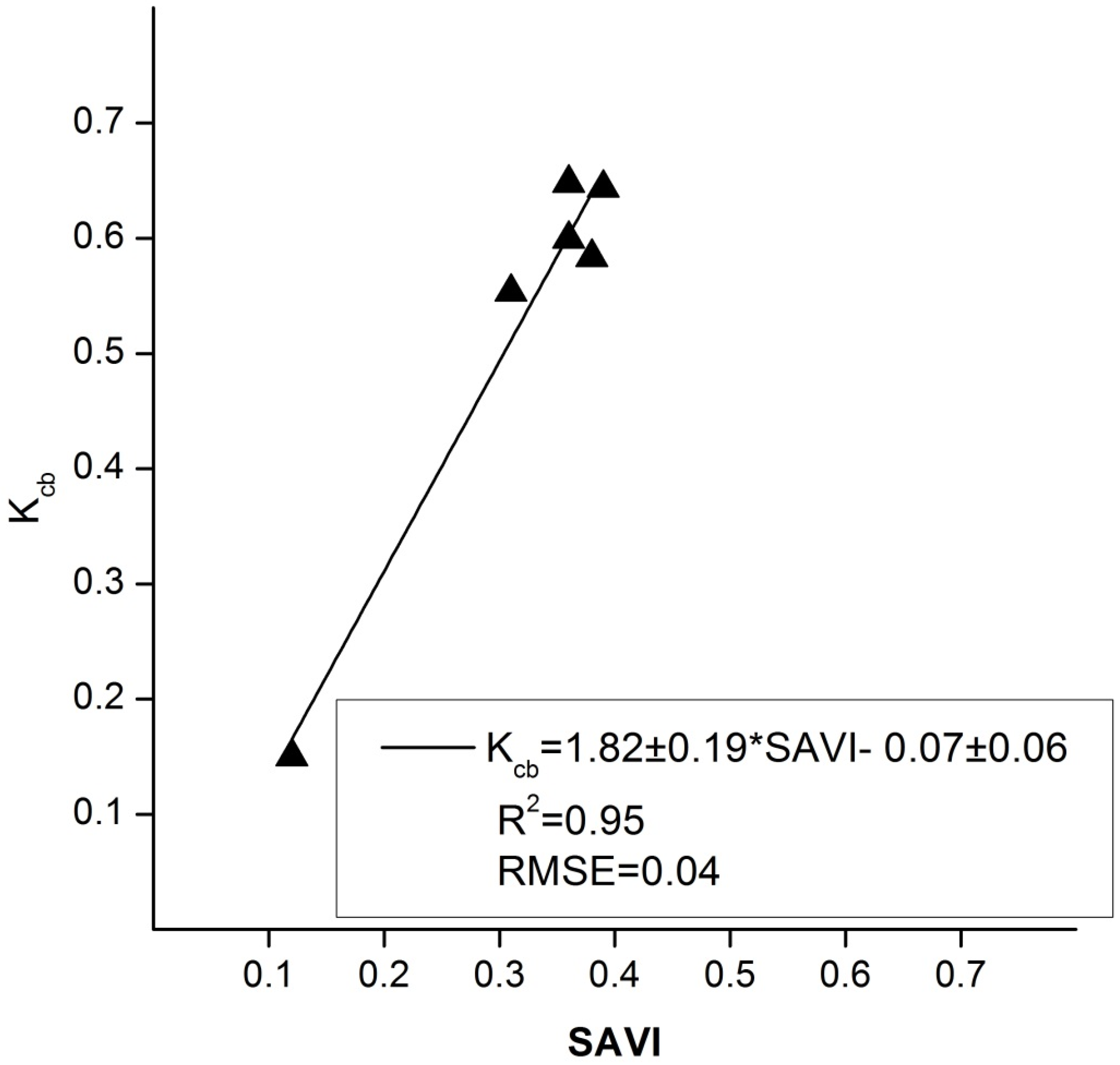
3.4. K_cb Modeled from SAVI

As mentioned previously, the K_cb values were obtained by the SAVI-K_cb linear relationship. This relationship was established between the observed maximum and minimum K_cb and their corresponding maximum and minimum values of SAVI as suggested by previous studies [8,19,26]. The average maximum SAVI was 0.37 at effective full cover when the inter-row weeds were dead, and its corresponding average maximum K_cb was 0.61. The dates that achieved these requirements were 1 January 2011, 27 November 2012, 30 January 2013, 15 February 2013 and 19 March 2013. On the other hand, the minimum SAVI value was 0.12 averaged from bare soil next to the study site, and its corresponding minimum K_cb was 0.15, which was taken from FAO-56 [3] for apple trees after leaf drop over dead ground cover or bare soil because the evaluated orchard presented active weeds after leaf drop until December. The resulting equation for the study apple orchard is shown in Figure 6. The SAVI-K_cb relationship resulted in a high coefficient of determination (R² = 0.95).

Previous efforts have reported VI-K_cb linear relationships for several herbaceous crops, such as corn, wheat, cotton, potato, sugar beet and garlic [6,15,19,24,25,26,27,66], however there are few studies for fruit trees. In that regard, the SAVI-K_cb and NDVI-K_cb linear relationships for vineyards have been reported by [8,20], whereas [27] recently applied linear relationships for mandarin, olive and peach and concluded that additional research with other crops would be desirable.

Since the relationship between VI and crop coefficient was based on the basal crop coefficient K_cb, that is defined as the ratio of the crop evapotranspiration over the reference evapotranspiration when the soil surface is dry but transpiration is occurring at potential rate [3], the value of K_cb is only affected by the canopy development. The effect of the soil moisture in the plant transpiration is provided by the water stress coefficient, while the effect of soil moisture in surface evaporation is provided by the soil evaporation coefficient. The relationship presented in Figure 6 was used during the whole growing season. Unfortunately, K_cb-SAVI pairs during the development and late-season growth stages were not available to discuss in depth the possible variations in this relationship due to the various crop growth stages and the understory vegetation effect. Nevertheless, previous works indicated a good correlation between K_cb or related parameters and VI during the entire growing season for vineyard [8] and wheat [67]. It should be noted the similarity between the apple relationship obtained in this work and the previous relationship reported by [8] for a row structured fruit orchard (vineyard). Although the development and analysis of specific relationships for new crops or canopies with different management are always recommended, the similarities founded in this study point to the evaluation of previous equations for the assessment of ET_c and irrigation requirements in several fruit trees.

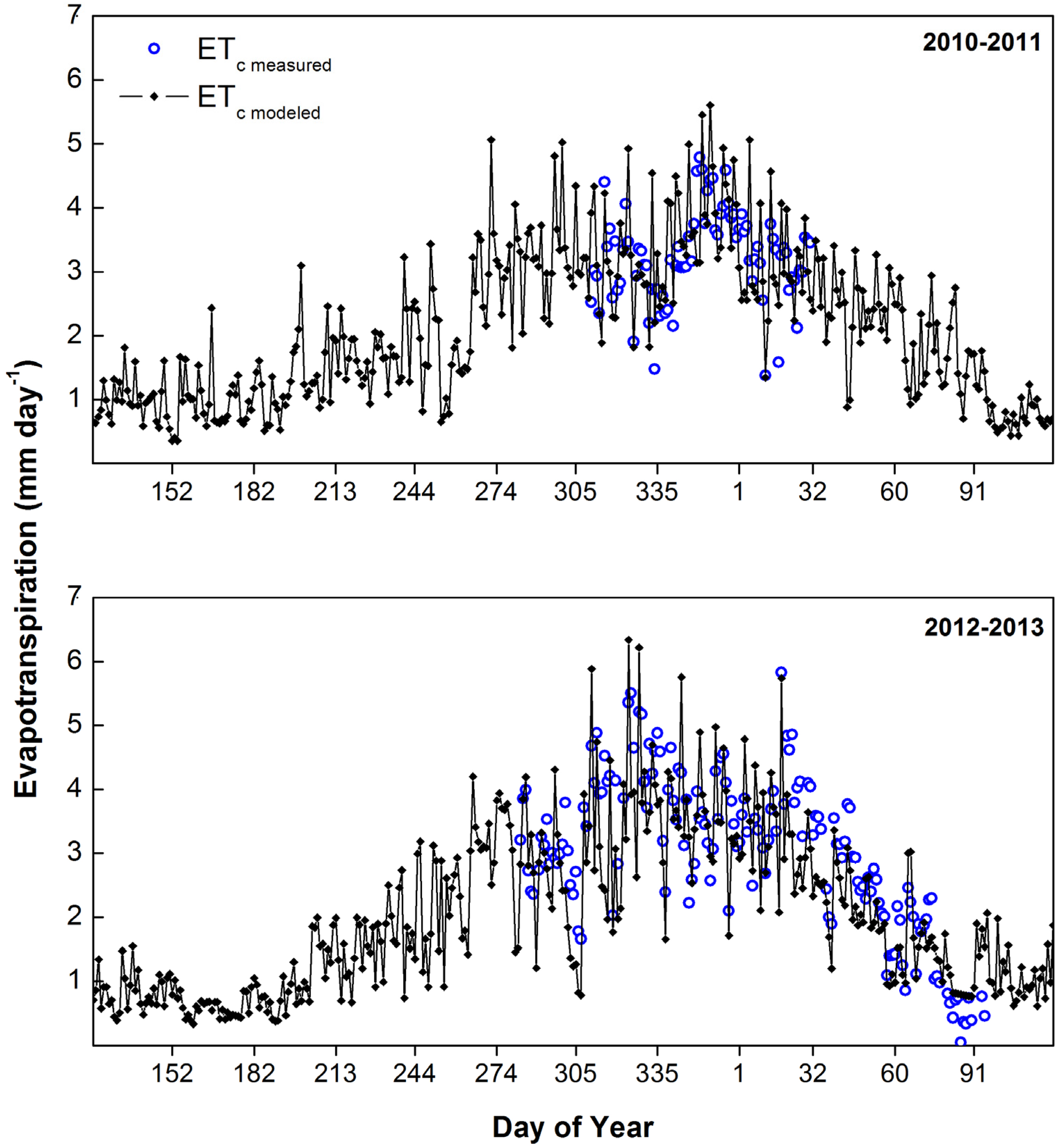
3.5. Evaluation of the One Layer Soil Water Balance Model for Estimating ET_c

The remote sensing-based water balance was applied, assimilating the reflectance based K_cb values, meteorological data and applied irrigation depths doses and dates at a daily scale. The modeled and measured ET_c values were compared during the midseason for both campaigns (Figure 7). The results at the daily scale indicate a reasonable agreement between the observed and modeled ET_c values, with an RMSE lower than 0.78 mm·day⁻¹ for both analyzed campaigns, which is equivalent to relative errors of 25%. Similar values of relative RMSE of daily ET_c (19%–27%) was also reported by [56] for a land cover of annual crops mainly. The general agreement was slightly better for the 2012–2013 campaign with an RMSE of 0.74 mm·day⁻¹ and an index of agreement (d) of 0.90 (

Table 3. Statistical measures for the comparison between the measured and modeled daily crop evapotranspiration using the remote sensing-based water balance model.

Growing Season	Daily Values
	RMSE (mm·day−1)	MBE (mm·day−1)	MAE (mm·day−1)	d	Observed Average (mm)	Relative RMSE	Relative MAE
2010–2011	0.78	0.13	0.62	0.73	3.24	0.24	0.19
2012–2013	0.74	−0.24	0.59	0.90	3.01	0.25	0.20

).

As described in previous applications of the remote sensing-based water balance model [8,59], the greater discrepancies between modeled and measured ET_c were found after precipitation and irrigation events. Wetting events produced an overestimation of daily ET_c due to bare soil evaporation that are not adequately simulated by the dual approach at a daily scale, but the total amount for longer periods seems to be properly modeled [36,37]. The comparison of ET_c for a weekly period indicated a considerably better agreement for both growing seasons, reducing the RMSE to values lower than 0.60 mm·day⁻¹ in both campaigns, which mean a relative error less than 20% (

Table 4. Statistical measures for the comparison between the measured and modeled weekly crop evapotranspiration using the remote sensing-based water balance model.

Growing Season	Weekly Values
	RMSE (mm·day−1)	MBE (mm·day−1)	MAE (mm·day−1)	d	Observed Average (mm)	Relative RMSE	Relative MAE
2010–2011	0.32	0.10	0.25	0.88	3.24	0.10	0.08
2012–2013	0.60	−0.26	0.47	0.92	3.01	0.20	0.16

). The improvement of the model performance on a weekly basis was due to several reasons as the reduction of the effect of meteorological conditions in the values of K_c [49] and the improvement of the precision of the top soil evaporation sub-model when the results are analyzed for weekly or greater time periods [37]. This improvement in the model performance was greater in the 2010–2011 campaign because the canopy development was lower during all the season resulting in a greater influence of the soil evaporation component. In addition, a weekly scheduling is a common practice and an adequate time lapse used in commercial orchards for the assessment and application of irrigation needs. Another factor that could explain the difference between the measured and modeled values of ET_c is the flux source area measured by eddy covariance system which depends of wind direction, also observed by [59] in olives. The different condition of the large area measured by eddy covariance system could include information from irrigation subunits with different irrigation timing (wet and dry) that could differ from the model inputs. The modeled area only included the subunit close to the eddy station (wet or dry).

Most of the works addressing the remote sensing-based water balance over row structured fruit trees have been done over vineyard, olives or other fruit than apple. Here, satellite-based crop coefficient and ET_c for apple orchard was reported and the model accuracy was compared with previous works that estimated ET_c for similar canopies using satellite data. The RMSEs obtained in this study for both growing seasons were lower than the range reported by [31] (0.9–1.0 mm·day⁻¹) for a land cover roughly classified as apple orchard (4.5 m height) with dispersed crops (wheat) using visible, near- and thermal-infrared data from MODIS products. Working in similar canopies like vineyards on a trellis system [30] obtained an RMSE equal to 0.45 and 0.76 mm·day⁻¹ during two consecutive growing seasons comparing EC measurements and ET_c derived from a remote sensing-based water balance, using the relationship between NDVI and the single crop coefficient K_c. For a variety of rainfed and irrigation vineyards, reference [68] obtained an RMSE lower than 0.65 mm·day⁻¹ for each analyzed campaign using a satellite-based crop coefficient and one layer soil water balance. In a row structured vineyard, reference [69] obtained an RMSE of 0.47 mm·day⁻¹ (17% of the measured values) using the single crop coefficient approach based on the FAO-56 tabulated coefficients. Additionally, the authors reported an RMSE of 0.37 mm·day⁻¹ (13% of the measured values) by dual crop coefficient approach combined with sap-flow techniques. A similar range of the RMSE for ET_c estimations using the crop coefficient vs. vegetation index relationship was also reported for peach (0.9 mm·day⁻¹) and olive (0.32–0.73 mm·day⁻¹) [27].

In addition, we want to highlight the possible limitation of the FAO-56 soil water balance model for the assessment of the root zone water depletion and stress coefficient in the present conditions, that is a drip irrigated apple orchard with active inter-row weeds during the initial and crop development growth stages. Firstly, the model considered the whole area as equally wetted and explored by the roots of the apple trees. However, for widely spaced crops as apple trees, drip-irrigation systems normally wet only a portion of the horizontal, cross-sectional area of soil [70]. Previous studies have demonstrated that some fruit trees, such as apple, kiwifruit and olive, can modify their pattern of water uptake in preference to roots placed in wet soil bulb [71,72,73]. Specifically, in mature apple trees, reference [71] observed that 70% of tree water uptake occurred in the top 0.4 m, because there were many fine roots near the soil surface. These studies indicate that apple trees are able to increase uptake from wet parts of the soil while reducing uptake from the dry parts of the root zone. In our study, the moisture sensors buried at the center of the inter-row showed that this area was not affected by irrigation events due to a combination of irrigation amounts, the location of the drip system and soil texture. This partial allocation of water amounts in the soil area could result in an overestimation of the water stress conditions simulated by the model, which distributed the irrigation water in the whole area. In other words, the simulation results in a misrepresentation of the water stress conditions that might not match the actual conditions. Secondly, the senescence of the weeds in the center of the alley during the midseason indicated that they did not use the irrigation water in this area. Nevertheless, during the initial and crop development growth stages, the soil water balance based on medium resolution satellite data will result in K_cb values which consider the transpiration of apple tree and weeds. Additional research would be desirable to achieve a separated water balances [59,74]—incorporating high resolutions satellite data—for the areas affected and non-affected by irrigation to obtain an accurate estimation of ET_c and optimize water management in orchards.

The remote sensing-based water balance model was inverted to estimate the optimum irrigation requirements according to the proposed formulation and constraints in reference to the maximum daily irrigation dose. The modeled irrigation water needs to avoid water stress were 457 in 2010–2011 and 412 mm in 2012–2013. These requirements resulted from the combination of ET_o, precipitation and K_c values for the each growing season (September to May). The accumulated ET_o during 2010–2011 growing season was higher than 2012–2013 growing season (975 and 875 mm, respectively), whereas rainfall was lower (255 and 373 mm, respectively).

On the other hand, the midseason K_c values were higher for the second growing season (0.63 and 0.73 for 2010–2011 and 2012–2013 growing seasons, respectively) due to a greater vegetation cover attributed to the orchard age. The modeled irrigation requirements are lower than the irrigation applied by the grower for both seasons (547 mm and 439 mm in 2010–2011 and 2012–2013 season, respectively). Even though the amount of irrigation applied by the grower was greater than the modeled one, a reduction of the stress coefficient, and, thus, K_c value in precise moments showed that irrigation timing was inadequate. In addition, the deep percolation observed with the grower irrigation was greater than the modeled one due to irrigation applied closer to precipitation events. Hence, the results indicate a potential improvement in the irrigation scheduling based on the model discussed here and the need to implement advisory services based on precise models, such as the methodology described in this paper.

4. Conclusions

The main results of this work have demonstrated that the satellite-based soil water balance was able to appropriately estimate crop evapotranspiration at field canopy scales and water depletion for an apple orchard during two growing seasons (2010–2011 and 2012–2013) in Maule Region, Chile. The RMSE between the measured and modeled daily ET_c was 0.78 and 0.74 mm·day⁻¹ for 2010–2011 and 2012–2013 seasons, respectively. However, weekly basis ET_c estimation improved the model performance avoiding the inaccurate simulation of peak values after wetting events (0.32 and 0.60 mm·day⁻¹ for the first and second seasons, respectively). The essential parameter to estimate ET_c was the reflectance-based crop coefficient obtained from satellite images, which responds to actual crop conditions in the field. This parameter was obtained using a linear relationship established between the basal crop coefficient and SAVI due to the similarity in the temporal pattern of both parameters. The linear relationship developed for the apple orchard resulted in a significant similarity with a previous relationship for row structured grapes. The results allow for the conclusion that the remote sensing-base water balance could be used as an operational tool to estimate ET_c and to plan the irrigation of apple orchards over large areas.

The continuous measurement of ET_c data during the entire growing season should be considered in future studies to evaluate the performance of the remote sensing-based water balance in all growth stages, as well as additional ground reflectance data at initial and crop development stages, which mostly occur during cloud cover intervals.

References

1. ODEPA-CIREN. Catastro Frutícola. Principales Resultados. Región del Maule; Ministerio de Agricultura: Santiago, Chile, 2013; p. 48.
2. Ministerio del Medio Ambiente. Segunda Comunicación Nacional de Chile ante la Convención Marco de las Naciones unidas sobre Cambio Climático; Ministerio del Medio Ambiente: Santiago, Chile, 2011; p. 289.
3. Allen, R.; Pereira, L.S.; Raes, D.; Smith, M. Crop Evapotranspiration: Guidelines for Computing Crop Requirements; Irrigation and Drainage Paper No. 56; FAO: Rome, Italy, 1998. [Google Scholar]
4. Doorenboos, J.; Pruitt, W.O. Guidelines for Predicting Crop Water Requirements, Irrigation and Drainage Paper 24; Land and Water Development Division, FAO: Rome, Italy, 1977; p. 144. [Google Scholar]
5. Wright, J.L. New evapotranspiration crop coefficients. J. Irrig. Drain. Div. 1982, 108, 57–74. [Google Scholar]
6. Bausch, W.C. Remote sensing of crop coefficients for improving the irrigation scheduling of corn. Agric. Water Manag. 1995, 27, 55–68. [Google Scholar] [CrossRef]
7. Allen, R.G.; Pereira, L.S. Estimating crop coefficients from fraction of ground cover and height. Irrig. Sci. 2009, 28, 17–34. [Google Scholar] [CrossRef]
8. Campos, I.; Neale, C.M.U.; Calera, A.; Balbontín, C.; González-Piqueras, J. Assessing satellite-based basal crop coefficients for irrigated grapes (Vitis vinifera L.). Agric. Water Manag. 2010, 98, 45–54. [Google Scholar] [CrossRef]
9. Fereres, E.; Goldhamer, D.A. Deciduous Fruit and Nut Trees. In Irrigation of Agricultural Crops—Monogr. 30; Stewart, B.A., Nielsen, D.R., Eds.; ASA: Madison, WI, USA, 1990; pp. 987–1017. [Google Scholar]
10. Bailey, R. Ecoclimatic zones of the earth. In Ecosystem Geography; Springer: New York, NY, USA, 2009; pp. 83–92. [Google Scholar]
11. Massman, W.J. Reply to comment by rannik on “a simple method for estimating frequency response corrections for eddy covariance systems”. Agric. For. Meteorol. 2001, 107, 247–251. [Google Scholar] [CrossRef]
12. Auzmendi, I.; Mata, M.; Lopez, G.; Girona, J.; Marsal, J. Intercepted radiation by apple canopy can be used as a basis for irrigation scheduling. Agric. Water Manag. 2011, 98, 886–892. [Google Scholar] [CrossRef]
13. Steduto, P.; Hsiao, T.C.; Fereres, E.; Raes, D. Crop yield response to water. In FAO Irrigation and Drainage Paper No. 66; FAO: Rome, Italy, 2012; p. 505. [Google Scholar]
14. Glenn, E.P.; Neale, C.M.U.; Hunsaker, D.J.; Nagler, P.L. Vegetation index-based crop coefficients to estimate evapotranspiration by remote sensing in agricultural and natural ecosystems. Hydrol. Processes 2011, 25, 4050–4062. [Google Scholar] [CrossRef]
15. Bausch, W.C.; Neale, C.M.U. Crop coefficients derived from reflected canopy radiation: A concept. Trans. ASAE 1987, 30, 703–709. [Google Scholar] [CrossRef]
16. Choudhury, B.; Ahmed, N.; Idso, S.; Reginato, R.; Daughtry, C. Relations between evaporation coefficients and vegetation indices studied by model simulations. Remote Sens. Environ. 1994, 50, 1–17. [Google Scholar] [CrossRef]
17. Heilman, J.L.; Heilman, W.E.; Moore, D.G. Evaluating the crop coefficient using spectral reflectance. Agron. J. 1982, 74, 967–971. [Google Scholar] [CrossRef]
18. Jackson, R.D.; Idso, S.B.; Reginato, R.J.; Pinter, P.J., Jr. Remotely sensed crop temperatures and reflectances as inputs to irrigation scheduling. In Irrigation and Drainage: Today’s Challenges; ASCE: New York, NY, USA, 1980; pp. 390–397. [Google Scholar]
19. Neale, C.M.U.; Bausch, W.C.; Heerman, D.F. Development of reflectance-based crop coefficients for corn. Trans. ASAE 1989, 32, 1891–1899. [Google Scholar] [CrossRef]
20. Consoli, S.; Barbagallo, S. Estimating water requirements of an irrigated mediterranean vineyard using a satellite-based approach. J. Irrig. Drain. Eng. 2012, 138, 896–904. [Google Scholar] [CrossRef]
21. Duchemin, B.; Hadria, R.; Erraki, S.; Boulet, G.; Maisongrande, P.; Chehbouni, a.; Escadafal, R.; Ezzahar, J.; Hoedjes, J.C.B.; Kharrou, M.H.; et al. Monitoring wheat phenology and irrigation in central morocco: On the use of relationships between evapotranspiration, crops coefficients, leaf area index and remotely-sensed vegetation indices. Agric. Water Manag. 2006, 79, 1–27. [Google Scholar] [CrossRef]
22. Er-Raki, S.; Chehbouni, A.; Guemouria, N.; Duchemin, B.; Ezzahar, J.; Hadria, R. Combining fao-56 model and ground-based remote sensing to estimate water consumptions of wheat crops in a semi-arid region. Agric. Water Manag. 2007, 87, 41–54. [Google Scholar] [CrossRef]
23. González-Dugo, M.P.; Escuin, S.; Cano, F.; Cifuentes, V.; Padilla, F.L.M.; Tirado, J.L.; Oyonarte, N.; Fernández, P.; Mateos, L. Monitoring evapotranspiration of irrigated crops using crop coefficients derived from time series of satellite images. II. Application on basin scale. Agric. Water Manag. 2013, 125, 92–104. [Google Scholar] [CrossRef]
24. González-Dugo, M.P.; Mateos, L. Spectral vegetation indices for benchmarking water productivity of irrigated cotton and sugarbeet crops. Agric. Water Manag. 2008, 95, 48–58. [Google Scholar] [CrossRef]
25. Hunsaker, D.J.; Pinter, P.J.; Barnes, E.M.; Kimball, B.A. Estimating cotton evapotranspiration crop coefficients with a multispectral vegetation index. Irrig. Sci. 2003, 22, 95–104. [Google Scholar] [CrossRef]
26. Jayanthi, H.; Neale, C.M.U.; Wright, J.L. Development and validation of canopy reflectance-based crop coefficient for potato. Agric. Water Manag. 2007, 88, 235–246. [Google Scholar] [CrossRef]
27. Mateos, L.; González-Dugo, M.P.; Testi, L.; Villalobos, F.J. Monitoring evapotranspiration of irrigated crops using crop coefficients derived from time series of satellite images. I. Method validation. Agric. Water Manag. 2013, 125, 81–91. [Google Scholar] [CrossRef]
28. Chen, J.M.; Chen, X.; Ju, W.; Geng, X. Distributed hydrological model for mapping evapotranspiration using remote sensing inputs. J. Hydrol. 2005, 305, 15–39. [Google Scholar] [CrossRef]
29. Cammalleri, C.; Ciraolo, G.; Minacapilli, M.; Rallo, G. Evapotranspiration from an olive orchard using remote sensing-based dual crop coefficient approach. Water Resour. Manag. 2013, 27, 4877–4895. [Google Scholar] [CrossRef]
30. Er-Raki, S.; Rodriguez, J.C.; Garatuza-Payan, J.; Watts, C.J.; Chehbouni, A. Determination of crop evapotranspiration of table grapes in a semi-arid region of northwest Mexico using multi-spectral vegetation index. Agric. Water Manag. 2013, 122, 12–19. [Google Scholar] [CrossRef]
31. Tang, R.; Li, Z.L.; Chen, K.S.; Zhu, Y.; Liu, W. Verification of land surface evapotranspiration estimation from remote sensing spatial contextual information. Hydrol. Processes 2012, 26, 2283–2293. [Google Scholar] [CrossRef]
32. CIREN. Descripciones de Suelos, Materiales y Simbolos. Estudio agrológico vii Region; Ministerio de Agricultura: Santiago, Chile, 1997; p. 659.
33. United States Soil Survey Staff. Soil Taxonomy. A basic System of Soil Classification for Making and Interpreting Soil Surveys; U.S. Department of Agriculture: Washington, DC, USA, 1999; p. 886.
34. Lauri, P.E.; Lespinasse, J.M. The Vertical Axis and Solaxe Systems in France; International Society for Horticultural Science (ISHS): Leuven, Belgium, 1998; pp. 287–296. [Google Scholar]
35. Campos, I.; Neale, C.M.U.; López, M.-L.; Balbontín, C.; Calera, A. Analyzing the effect of shadow on the relationship between ground cover and vegetation indices by using spectral mixture and radiative transfer models. J. Appl. Remote Sens. 2014, 8, 1–21. [Google Scholar] [CrossRef]
36. Muztiger, A.J.; Burt, C.M.; Howes, D.J.; Allen, R.G. Comparison of measured and fao 56 modeled evaporation from bare soil. J. Irrig. Drain.Eng. 2005, 131, 59–72. [Google Scholar]
37. Torres, E.A.; Calera, A. Bare soil evaporation under high evaporation demand: A proposed modification to the fao-56 model. Hydrol. Sci. J. 2010, 55, 303–315. [Google Scholar] [CrossRef]
38. Saxton, K.E.; Rawls, W.J.; Romberger, J.S.; Papendick, R.I. Estimating generalized soil-water characteristics from texture. Soil Sci. Soc. Am. J. 1986, 50, 1031–1036. [Google Scholar] [CrossRef]
39. Laubach, J.; Raschendorfer, M.; Kreilein, H.; Gravenhorst, G. Determination of heat and water vapour fluxes above a spruce forest by eddy correlation. Agric. For. Meteorol. 1994, 71, 373–401. [Google Scholar] [CrossRef]
40. Gash, J.H.C. Observations of turbulence downwind of a forest-heath interface. Bound.-Layer Meteorol. 1986, 36, 227–237. [Google Scholar] [CrossRef]
41. Li, S.; Kang, S.; Li, F.; Zhang, L.; Zhang, B. Vineyard evaporative fraction based on eddy covariance in an arid desert region of northwest China. Agric. Water Manag. 2008, 95, 937–948. [Google Scholar] [CrossRef]
42. Poblete-Echeverría, C.; Ortega-Farias, S. Estimation of actual evapotranspiration for a drip-irrigated merlot vineyard using a three-source model. Irrig. Sci. 2009, 28, 65–78. [Google Scholar] [CrossRef]
43. Baldocchi, D.; Rao, K.S. Intra-field variability of scalar flux densities across a transition between a desert and an irrigated potato field. Bound.-Layer Meteorol. 1995, 76, 109–136. [Google Scholar] [CrossRef]
44. Webb, E.K.; Pearman, G.I.; Leuning, R. Correction of flux measurements for density effects due to heat and water-vapor transfer. Q. J. R. Meteorol. Soc. 1980, 106, 85–100. [Google Scholar] [CrossRef]
45. Hui, D.; Wan, S.; Su, B.; Katul, G.; Monson, R.; Luo, Y. Gap-filling missing data in eddy covariance measurements using multiple imputation (MI) for annual estimations. Agric. For. Meteorol. 2004, 121, 93–111. [Google Scholar] [CrossRef]
46. Falge, E.; Baldocchi, D.; Olson, R.; Anthoni, P.; Aubinet, M.; Bernhofer, C.; Burba, G.; Ceulemans, R.; Clement, R.; Dolman, H.; et al. Gap filling strategies for long term energy flux data sets. Agric. For. Meteorol. 2001, 107, 71–77. [Google Scholar] [CrossRef]
47. Payero, J.O.; Neale, C.M.U.; Wright, J.L. Estimating soil heat flux for alfalfa and clipped tall fescue grass. Appl. Eng. Agric. 2005, 21, 401–409. [Google Scholar] [CrossRef]
48. Twine, T.E.; Kustas, W.P.; Norman, J.M.; Cook, D.R.; Houser, P.R.; Meyers, T.P.; Prueger, J.H.; Starks, P.J.; Wesely, M.L. Correcting eddy covariance flux underestimates over a grassland. Agric. For. Meteorol. 2000, 103, 279–300. [Google Scholar] [CrossRef]
49. Martínez-Cob, A.; Faci, J.M. Evapotranspiration of an hedge-pruned olive orchard in a semiarid area of ne Spain. Agric. Water Manag. 2010, 97, 410–418. [Google Scholar] [CrossRef] [Green Version]
50. Adler-Golden, S.M.; Matthew, M.W.; Bernstein, L.S.; Levine, R.Y.; Berk, A.; Richtsmeier, S.C.; Acharya, P.K.; Anderson, G.P.; Felde, G.; Gardner, J.; et al. Atmospheric correction for short-wave spectral imagery based on MODTRAN4. SPIE Proc. Imaging Spectrom. 1999, 3753, 61–69. [Google Scholar]
51. Berk, A.; Bernstein, L.S.; Robertson, D.C. Modtran: A Moderate Resolution Model for Lowtran 7; GL-TR-89-0122; Air Force Geophysics Laboratory: Bedford, MA, USA, 1989. [Google Scholar]
52. Vermote, E.F.; Tanré, D.; Deuzé, J.L.; Herman, M.; Morcrette, J.J. Second simulation of the satellite signal in the solar spectrum, 6s: An overview. IEEE Trans. Geosci. Remote Sens. 1997, 35, 675–686. [Google Scholar] [CrossRef]
53. Chander, G.; Markham, B.L.; Helder, D.L. Summary of current radiometric calibration coefficients for Landsat mss, TM, ETM+, and EO-1 ALI sensors. Remote Sens. Environ. 2009, 113, 893–903. [Google Scholar] [CrossRef]
54. Huete, A.R. A soil-adjusted vegetation index (SAVI). Remote Sens. Environ. 1988, 25, 295–309. [Google Scholar] [CrossRef]
55. Willmott, C. Some comments on the evaluation of model performance. Bull. Am. Meteorol. Soc. 1982, 63, 1309–1313. [Google Scholar] [CrossRef]
56. Tang, R.; Li, Z.-L.; Sun, X. Temporal upscaling of instantaneous evapotranspiration: An intercomparison of four methods using eddy covariance measurements and MODIS data. Remote Sens. Environ. 2013, 138, 102–118. [Google Scholar] [CrossRef]
57. Marsal, J.; Lopez, G.; Mata, M.; Arbones, A.; Girona, J. Recommendations for water conservation in peach orchards in mediterranean climate zones using combined regulated deficit irrigation. Acta Hortic. 2004, 664, 391–397. [Google Scholar] [CrossRef]
58. O'Connell, M.G.; Goodwin, I. Responses of “pink lady” apple to deficit irrigation and partial rootzone drying: Physiology, growth, yield, and fruit quality. Aust. J. Agric. Res. 2007, 58, 1068–1076. [Google Scholar] [CrossRef]
59. Er-Raki, S.; Chehbouni, A.; Boulet, G.; Williams, D.G. Using the dual approach of FAO-56 for partitioning et into soil and plant components for olive orchards in a semi-arid region. Agric. Water Manag. 2010, 97, 1769–1778. [Google Scholar] [CrossRef] [Green Version]
60. Ortega-Farias, S.; Carrasco, M.; Olioso, A.; Acevedo, C.; Poblete, C. Latent heat flux over cabernet sauvignon vineyard using the shuttleworth and wallace model. Irrig. Sci. 2007, 25, 161–170. [Google Scholar] [CrossRef]
61. Stoy, P.C.; Mauder, M.; Foken, T.; Marcolla, B.; Boegh, E.; Ibrom, A.; Arain, M.A.; Arneth, A.; Aurela, M.; Bernhofer, C.; et al. A data-driven analysis of energy balance closure across fluxnet research sites: The role of landscape scale heterogeneity. Agric. For. Meteorol. 2013, 171–172, 137–152. [Google Scholar] [CrossRef]
62. Tang, R.; Li, Z.-L.; Jia, Y.; Li, C.; Chen, K.-S.; Sun, X.; Lou, J. Evaluating one- and two-source energy balance models in estimating surface evapotranspiration from landsat-derived surface temperature and field measurements. Int. J. Remote Sens. 2013, 34, 3299–3313. [Google Scholar] [CrossRef]
63. Katul, G.; Hsieh, C.-I.; Bowling, D.; Clark, K.; Shurpali, N.; Turnipseed, A.; Albertson, J.; Tu, K.; Hollinger, D.; Evans, B. Spatial variability of turbulent fluxes in the roughness sublayer of an even-aged pine forest. Bound.-Layer Meteorol. 1999, 93, 1–28. [Google Scholar] [CrossRef]
64. Consoli, S.; Vanella, D. Comparisons of satellite-based models for estimating evapotranspiration fluxes. J. Hydrol. 2014, 513, 475–489. [Google Scholar] [CrossRef]
65. Girona, J.; Campo, J.; Mata, M.; Lopez, G.; Marsal, J. A comparative study of apple and pear tree water consumption measured with two weighing lysimeters. Irrig. Sci. 2011, 29, 55–63. [Google Scholar] [CrossRef]
66. Hunsaker, D.J.; Pinter, P.J.; Kimball, B.A. Wheat basal crop coefficients determined by normalized difference vegetation index. Irrig. Sci. 2005, 24, 1–14. [Google Scholar] [CrossRef]
67. López-Urrea, R.; Montoro, A.; González-Piqueras, J.; López-Fuster, P.; Fereres, E. Water use of spring wheat to raise water productivity. Agric. Water Manag. 2009, 96, 1305–1310. [Google Scholar] [CrossRef]
68. Campos, I.; Balbontín, C.; González-Piqueras, J.; González-Dugo, M.P.; Neale, C.M.; Calera, A. Combining a water balance model with evapotranspiration measurements to estimate total available soil water in irrigated and rainfed vineyards. Agric. Water Manag. 2016, 165, 141–152. [Google Scholar] [CrossRef]
69. Poblete-Echeverría, C.; Ortega-Farias, S. Evaluation of single and dual crop coefficients over a drip-rrigated merlot vineyard (Vitis vinifera L.) using combined measurements of sap flow sensors and an eddy covariance system. Aust. J. Grape Wine Res. 2013, 19, 249–260. [Google Scholar] [CrossRef]
70. Keller, J.; Bliesner, R.D. Sprinkle and Trickle Irrigation; Van Nostrand Reinhold: Princeton, NJ, USA, 1990. [Google Scholar]
71. Green, S.; Clothier, B. The root zone dynamics of water uptake by a mature apple tree. Plant Soil 1999, 206, 61–77. [Google Scholar] [CrossRef]
72. Green, S.R.; Clothier, B.E. Root water uptake by kiwifruit vines following partial wetting of the root zone. Plant Soil 1995, 173, 317–328. [Google Scholar] [CrossRef]
73. Moreno, F.; Fernandez, J.E.; Clothier, B.E.; Green, S.R. Transpiration and root water uptake by olive trees. Plant Soil 1996, 184, 85–96. [Google Scholar] [CrossRef]
74. Palomo, M.J.; Moreno, F.; Fernández, J.E.; Díaz-Espejo, A.; Girón, I.F. Determining water consumption in olive orchards using the water balance approach. Agric. Water Manag. 2002, 55, 15–35. [Google Scholar] [CrossRef]
Figure 1. Location of the experimental apple orchard, the eddy covariance flux station and the surrounding fields.
Remotesensing 08 00253 g001
Figure 2. Daily reference evapotranspiration (FAO-56 Penman–Monteith ETo), rainfall and irrigation during the 2010–2011 and 2012–2013 growing seasons.
Remotesensing 08 00253 g002
Figure 3. Overall comparison between sensible heat flux plus latent heat flux (LE + H) versus net radiation minus soil heat flux (Rn − G) in a drip-irrigated apple orchard during the 2010–11 and 2012–13 growing seasons.
Remotesensing 08 00253 g003
Figure 4. Temporal evolution of measured and modeled evapotranspiration for the drip-irrigated apple orchard (ETc) during the 2010–11 and 2012–13 seasons.
Remotesensing 08 00253 g004
Figure 5. Evolution of the soil adjusted vegetation index (SAVI) and the basal crop coefficient from the eddy covariance system (EC) for the drip‑irrigated apple orchard during the 2010–11 and 2012–13 growing seasons. Shaded areas represent the midseason growth stages. Unfilled squares represent the period with apple-weeds cover mixture.
Remotesensing 08 00253 g005
Figure 6. Kcb-SAVI linear relationship for the studied apple orchard. Kcb values at effective full cover correspond to the apple canopy without weeds.
Remotesensing 08 00253 g006
Figure 7. Daily and weekly values of measured and modeled actual evapotranspiration (ETc) for both seasons. Modeled ETc values were simulated using the remote sensing-based water balance models.
Remotesensing 08 00253 g007