
Evaluation of an Airborne Remote Sensing Platform Consisting of Two Consumer-Grade Cameras for Crop Identification

 ,
,
Abstract
:
1. Introduction
2. Materials and Methods
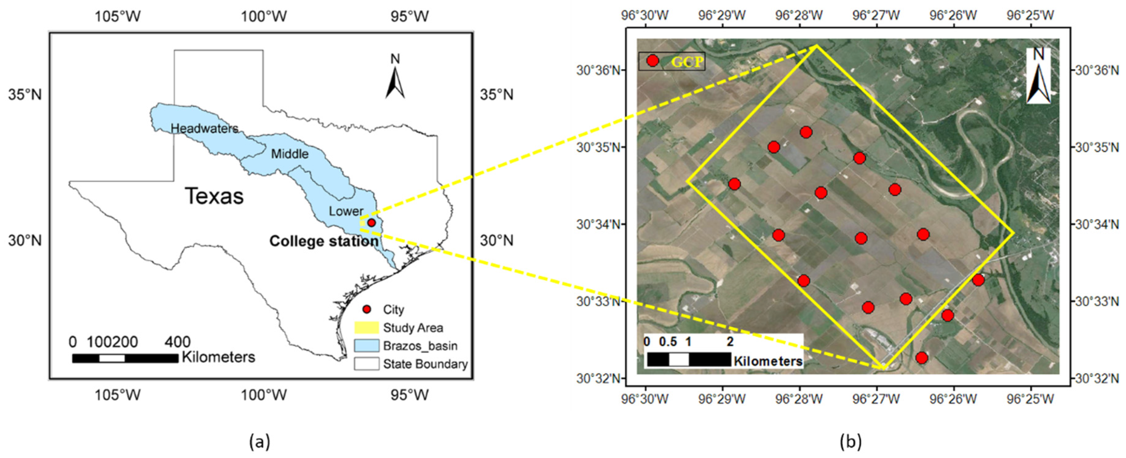
2.1. Study Area
2.2. Imaging System and Airborne Image Acquisition
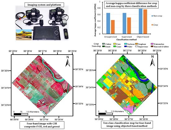
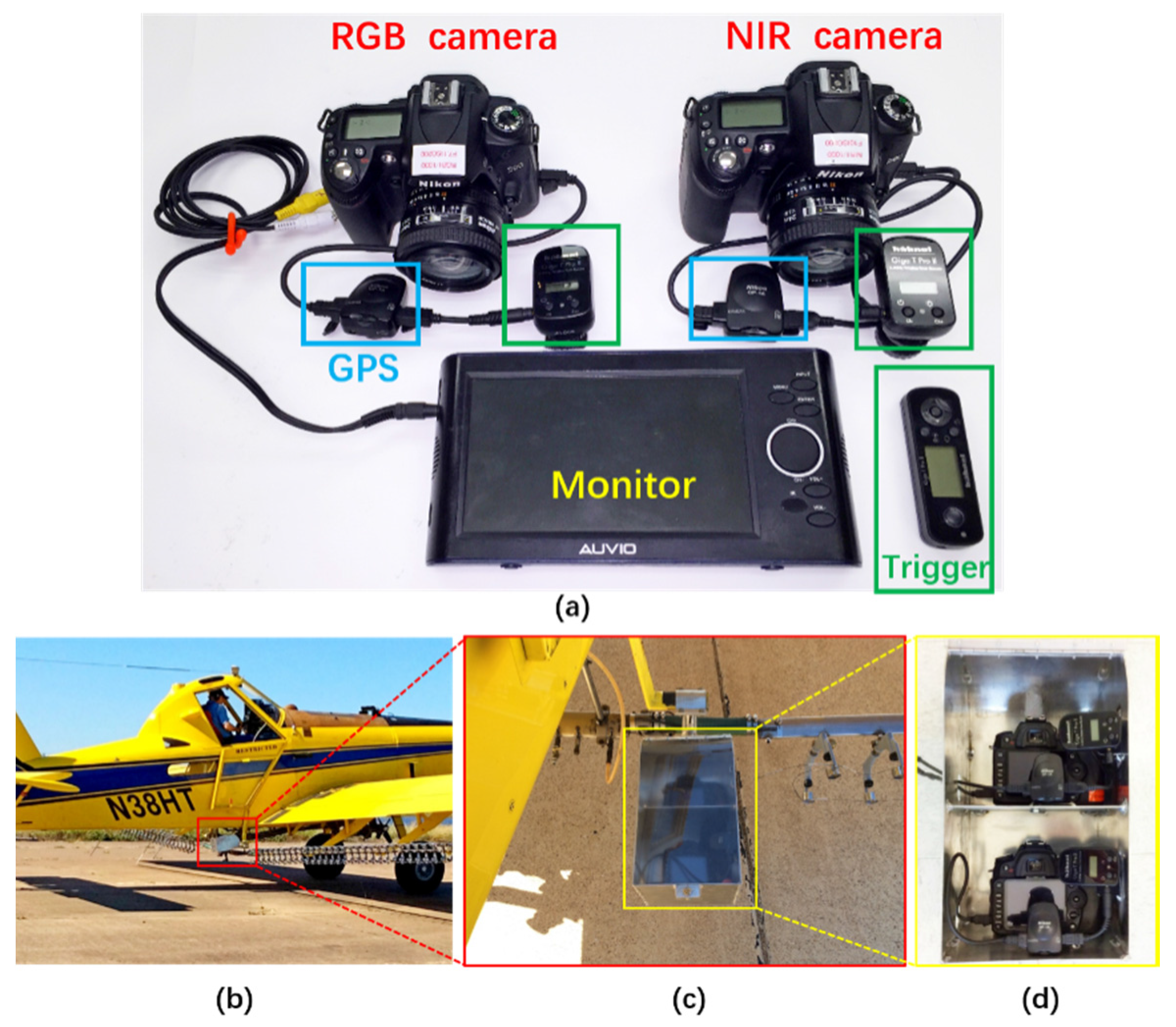
2.2.1. Imaging System and Platform
2.2.2. Spectral Characteristics of the Cameras
2.3. Image Acquisition and Pre-Processing
2.3.1. Airborne Image Acquisition
2.3.2. Image Pre-Processing
2.4. Crop Identification
2.4.1. Pixel-Based Classification
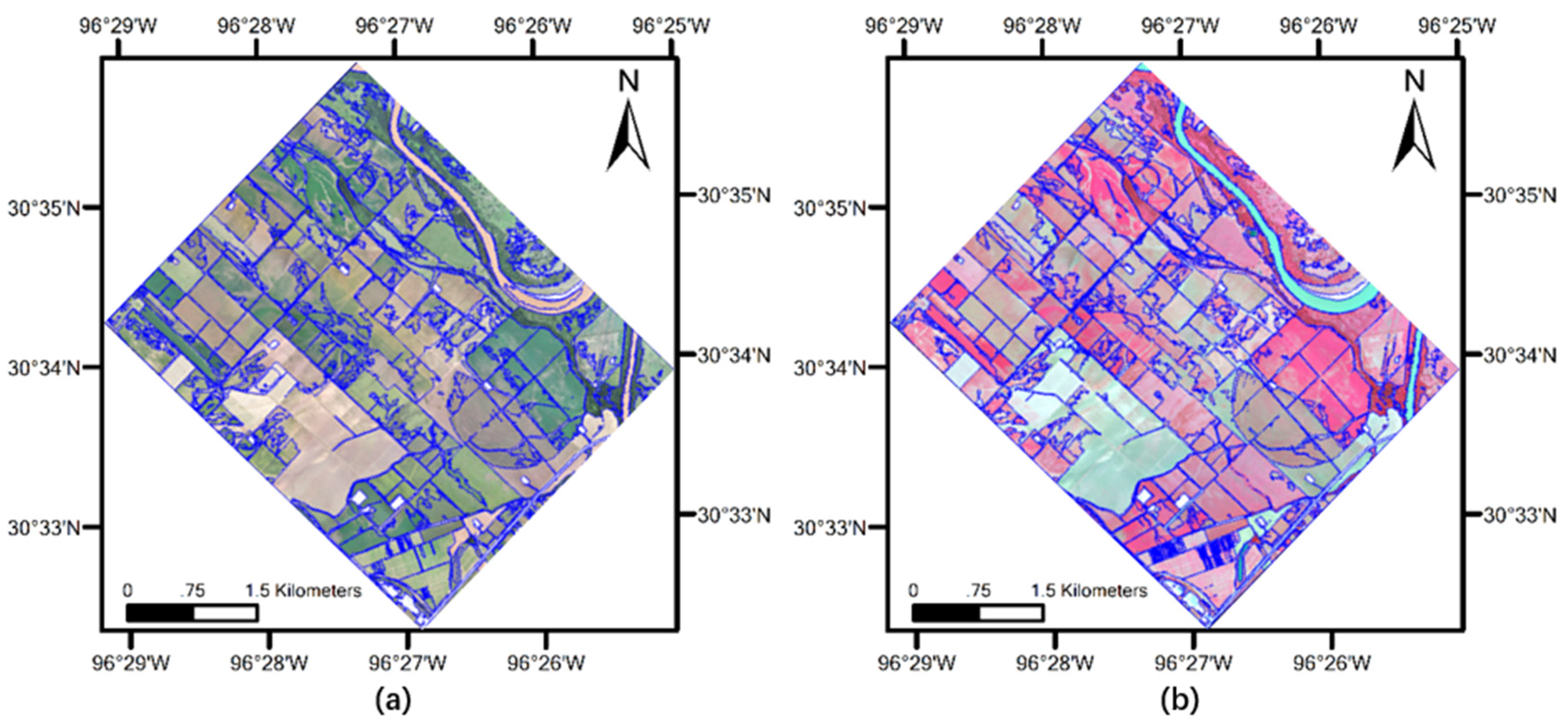
2.4.2. Object-Based Classification
2.5. Accuracy Assessment
3. Results
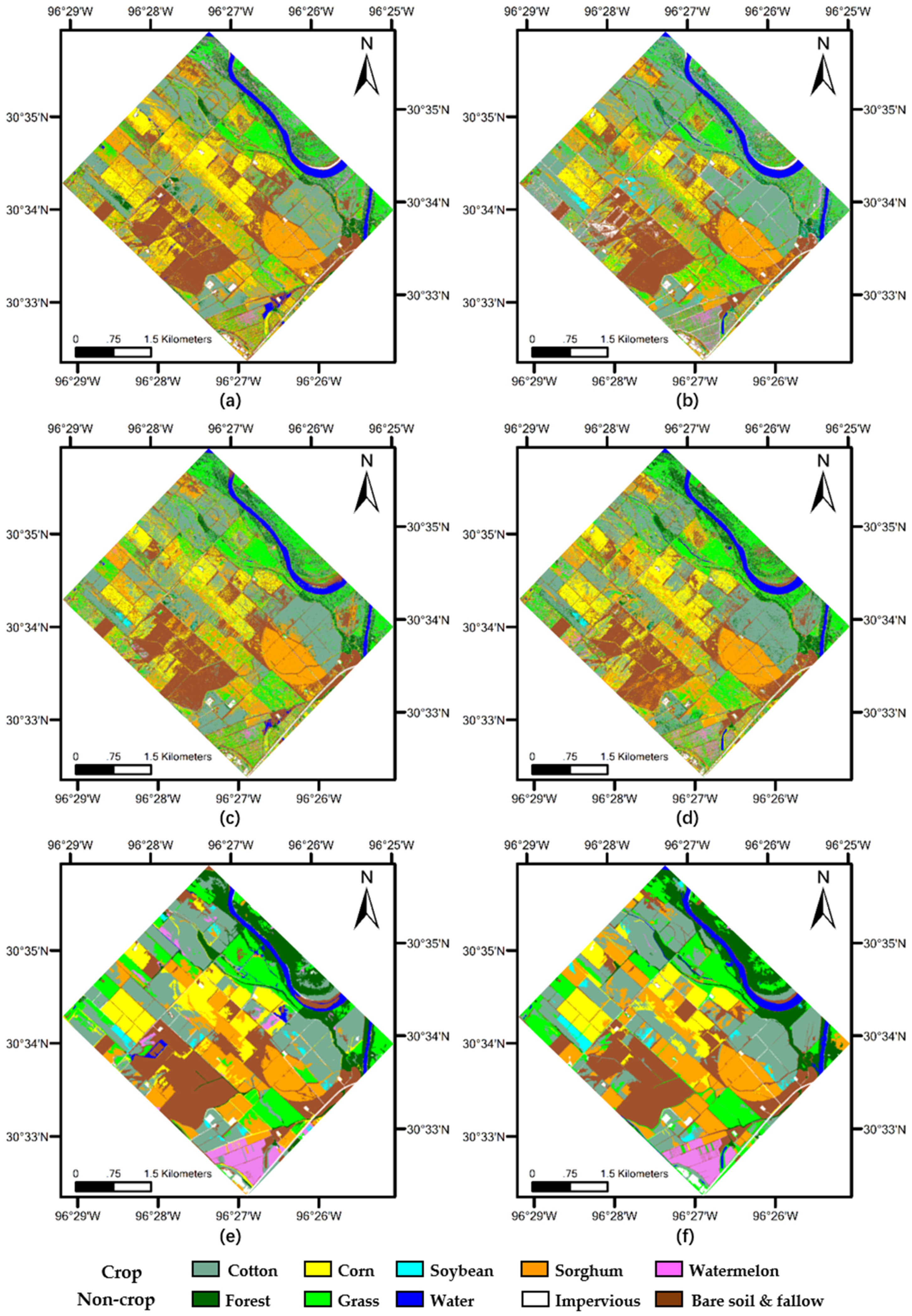
3.1. Classification Results
3.2. Accuracy Assessment
4. Discussion
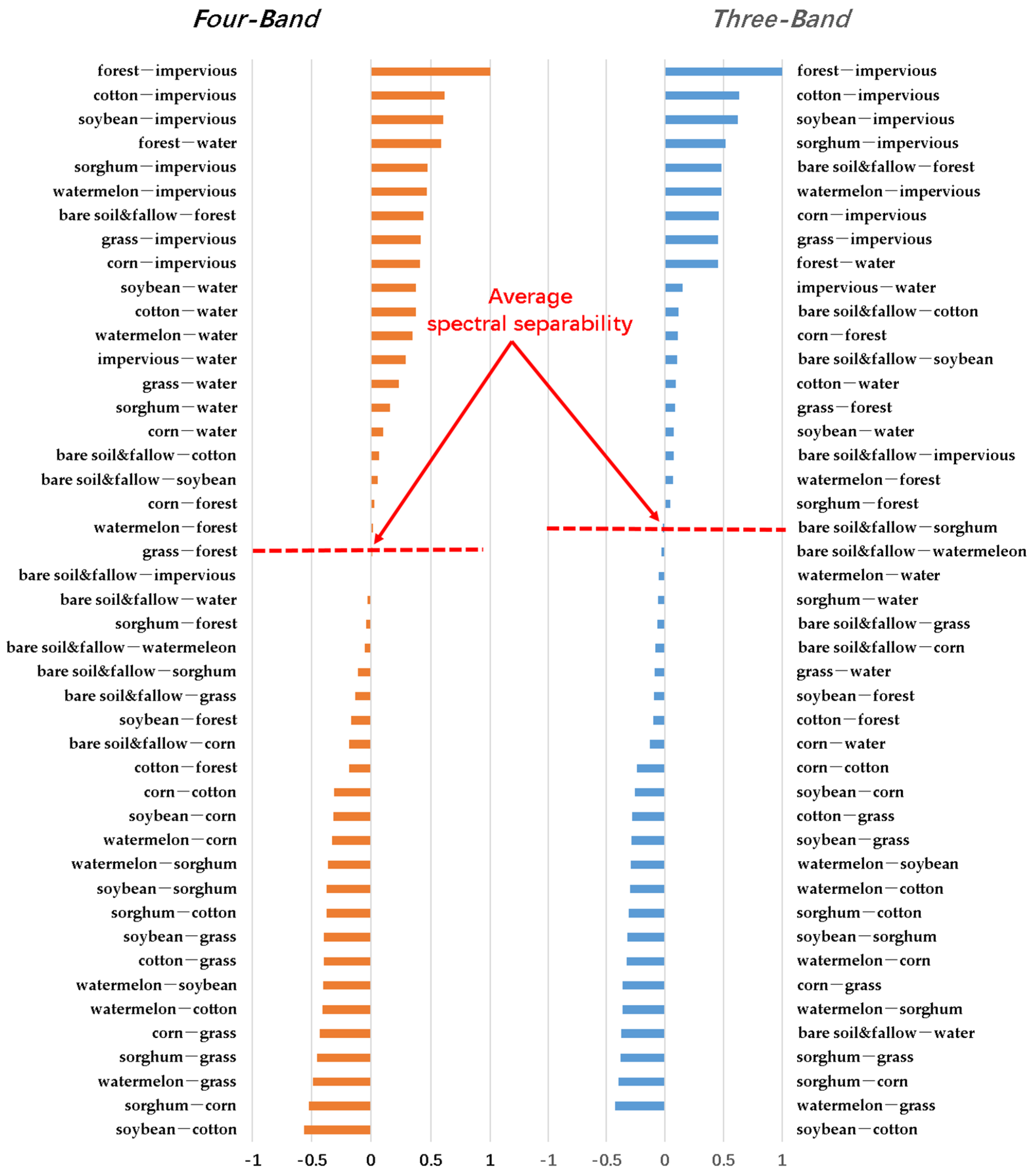
4.1. Importance of NIR Band
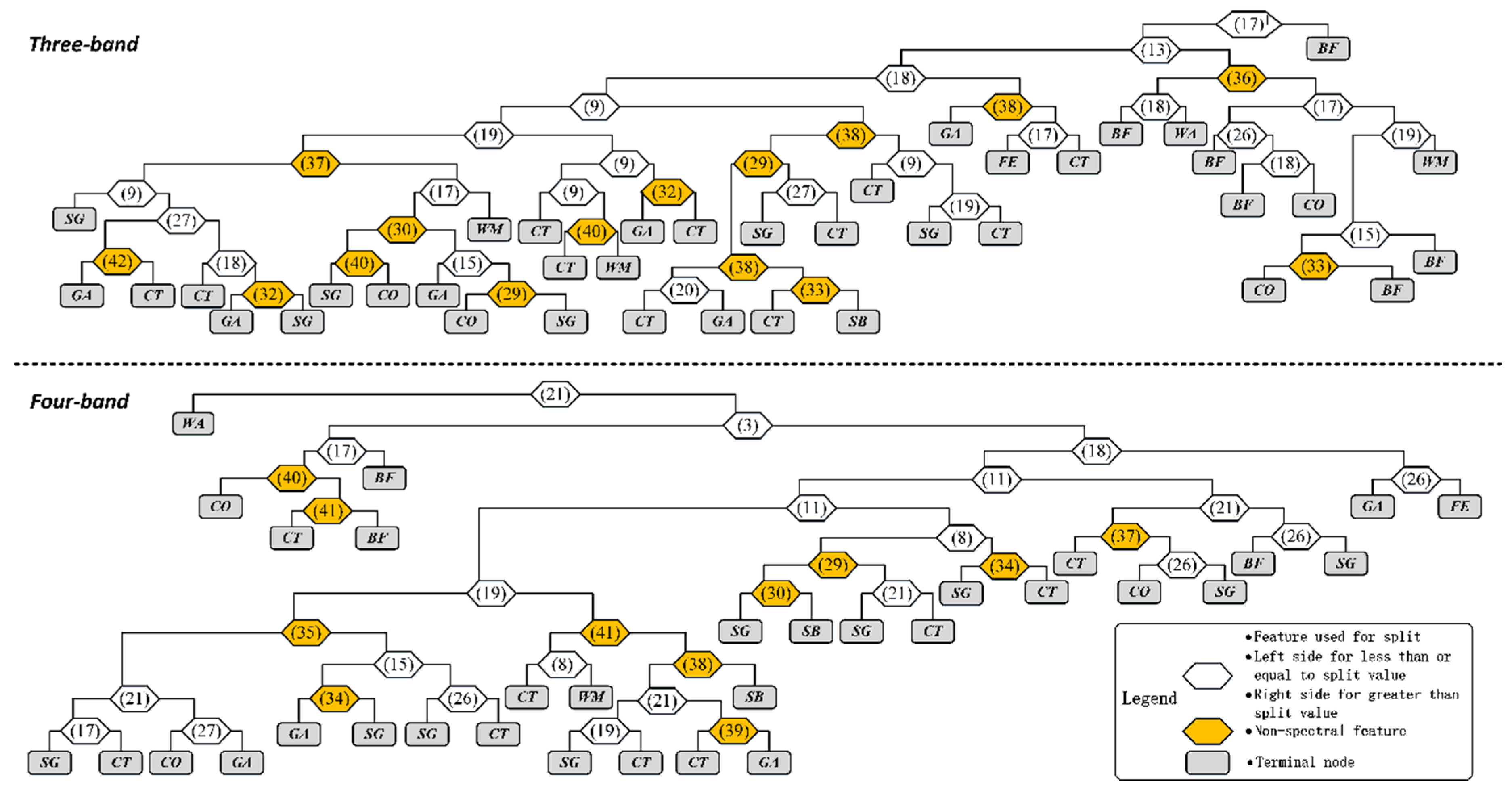
4.2. Importance of Object-Based Method
4.3. Importance of Classification Groupings
4.4. Implications for Selection of Imaging Platform and Classification Method
5. Conclusions
Acknowledgments
Author Contributions
Conflicts of Interest
Disclaimer
References
- Mulla, D.J. Twenty five years of remote sensing in precision agriculture: Key advances and remaining knowledge gaps. Biosyst. Eng. 2013, 114, 358–371. [Google Scholar] [CrossRef]
- Bauer, M.E.; Cipra, J.E. Identification of agricultural crops by computer processing of ERTS MSS data. In Proceedings of the Symposium on Significant Results Obtained from the Earth Resources Technology Satellite-1, New Carollton, IN, USA, 5–9 March 1973; pp. 205–212.
- Colomina, I.; Molina, P. Unmanned aerial systems for photogrammetry and remote sensing: A review. ISPRS J. Photogramm. Remote Sens. 2014, 92, 79–97. [Google Scholar] [CrossRef]
- Zhang, C.; Kovacs, J.M. The application of small unmanned aerial systems for precision agriculture: A review. Precis. Agric. 2012, 13, 693–712. [Google Scholar] [CrossRef]
- Watts, A.C.; Ambrosia, V.G.; Hinkley, E.A. Unmanned aircraft systems in remote sensing and scientific research: Classification and considerations of use. Remote Sens. 2012, 4, 1671–1692. [Google Scholar] [CrossRef]
- Araus, J.L.; Cairns, J.E. Field high-throughput phenotyping: The new crop breeding frontier. Trends Plant Sci. 2014, 19, 52–61. [Google Scholar] [CrossRef] [PubMed]
- Quilter, M.C.; Anderson, V.J. Low altitude/large scale aerial photographs: A tool for range and resource managers. Rangel. Arch. 2000, 22, 13–17. [Google Scholar]
- Hunt, E., Jr.; Daughtry, C.; McMurtrey, J.; Walthall, C.; Baker, J.; Schroeder, J.; Liang, S. Comparison of remote sensing imagery for nitrogen management. In Proceedings of the Sixth International Conference on Precision Agriculture and Other Precision Resources Management, Minneapolis, MN, USA, 14–17 July 2002; pp. 1480–1485.
- Wellens, J.; Midekor, A.; Traore, F.; Tychon, B. An easy and low-cost method for preprocessing and matching small-scale amateur aerial photography for assessing agricultural land use in burkina faso. Int. J. Appl. Earth Obs. Geoinf. 2013, 23, 273–278. [Google Scholar] [CrossRef]
- Oberthür, T.; Cock, J.; Andersson, M.S.; Naranjo, R.N.; Castañeda, D.; Blair, M. Acquisition of low altitude digital imagery for local monitoring and management of genetic resources. Comput. Electron. Agric. 2007, 58, 60–77. [Google Scholar] [CrossRef]
- Hunt, E.R., Jr.; Cavigelli, M.; Daughtry, C.S.; Mcmurtrey, J.E., III; Walthall, C.L. Evaluation of digital photography from model aircraft for remote sensing of crop biomass and nitrogen status. Precis. Agric. 2005, 6, 359–378. [Google Scholar] [CrossRef]
- Chiabrando, F.; Nex, F.; Piatti, D.; Rinaudo, F. UAV and RPV systems for photogrammetric surveys in archaelogical areas: Two tests in the piedmont region (Italy). J. Archaeol. Sci. 2011, 38, 697–710. [Google Scholar] [CrossRef]
- Nijland, W.; de Jong, R.; de Jong, S.M.; Wulder, M.A.; Bater, C.W.; Coops, N.C. Monitoring plant condition and phenology using infrared sensitive consumer grade digital cameras. Agric. For. Meteorol. 2014, 184, 98–106. [Google Scholar] [CrossRef]
- Murakami, T.; Idezawa, F. Growth survey of crisphead lettuce (Lactuca sativa L.) in fertilizer trial by low-altitude small-balloon sensing. Soil Sci. Plant Nutr. 2013, 59, 410–418. [Google Scholar] [CrossRef]
- Yang, C.; Westbrook, J.K.; Suh, C.P.C.; Martin, D.E.; Hoffmann, W.C.; Lan, Y.; Fritz, B.K.; Goolsby, J.A. An airborne multispectral imaging system based on two consumer-grade cameras for agricultural remote sensing. Remote Sens. 2014, 6, 5257–5278. [Google Scholar] [CrossRef]
- Miller, C.D.; Fox-Rabinovitz, J.R.; Allen, N.F.; Carr, J.L.; Kratochvil, R.J.; Forrestal, P.J.; Daughtry, C.S.T.; McCarty, G.W.; Hively, W.D.; Hunt, E.R. Nir-green-blue high-resolution digital images for assessment of winter cover crop biomass. GISci. Remote Sens. 2011, 48, 86–98. [Google Scholar]
- Artigas, F.; Pechmann, I.C. Balloon imagery verification of remotely sensed phragmites australis expansion in an urban estuary of New Jersey, USA. Landsc. Urban Plan. 2010, 95, 105–112. [Google Scholar] [CrossRef]
- Yang, C.; Hoffmann, W.C. Low-cost single-camera imaging system for aerial applicators. J. Appl. Remote Sens. 2015, 9, 096064. [Google Scholar] [CrossRef]
- Wang, Q.; Zhang, X.; Wang, Y.; Chen, G.; Dan, F. The design and development of object-oriented uav image change detection system. In Geo-Informatics in Resource Management and Sustainable Ecosystem; Springer-Verlag: Berlin/Heidelberg, Germany, 2013; pp. 33–42. [Google Scholar]
- Diaz-Varela, R.; Zarco-Tejada, P.J.; Angileri, V.; Loudjani, P. Automatic identification of agricultural terraces through object-oriented analysis of very high resolution dsms and multispectral imagery obtained from an unmanned aerial vehicle. J. Environ. Manag. 2014, 134, 117–126. [Google Scholar] [CrossRef] [PubMed]
- Lelong, C.C.D. Assessment of unmanned aerial vehicles imagery for quantitative monitoring of wheat crop in small plots. Sensors 2008, 8, 3557–3585. [Google Scholar] [CrossRef]
- Liebisch, F.; Kirchgessner, N.; Schneider, D.; Walter, A.; Hund, A. Remote, aerial phenotyping of maize traits with a mobile multi-sensor approach. Plant Methods 2015, 11. [Google Scholar] [CrossRef] [PubMed]
- Labbé, S.; Roux, B.; Bégué, A.; Lebourgeois, V.; Mallavan, B. An operational solution to acquire multispectral images with standard light cameras: Characterization and acquisition guidelines. In Proceedings of the International Society of Photogrammetry and Remote Sensing Workshop, Newcastle, UK, 11–14 September 2007; pp. TS10:1–TS10:6.
- Lebourgeois, V.; Bégué, A.; Labbé, S.; Mallavan, B.; Prévot, L.; Roux, B. Can commercial digital cameras be used as multispectral sensors? A crop monitoring test. Sensors 2008, 8, 7300–7322. [Google Scholar] [CrossRef] [Green Version]
- Visockiene, J.S.; Brucas, D.; Ragauskas, U. Comparison of UAV images processing softwares. J. Meas. Eng. 2014, 2, 111–121. [Google Scholar]
- Pix4D. Getting GCPs in the Field or through Other Sources. Available online: https://support.pix4d.com/hc/en-us/articles/202557489-Step-1-Before-Starting-a-Project-4-Getting-GCPs-in-the-Field-or-Through-Other-Sources-optional-but-recommended- (accessed on 26 December 2015).
- Hexagon Geospatial. ERDAS IMAGINE Help. Automatic Tie Point Generation Properties. Available online: https://hexagongeospatial.fluidtopics.net/book#!book;uri=fb4350968f8f8b57984ae66bba04c48d;breadcrumb=23b983d2543add5a03fc94e16648eae7-b70c75349e3a9ef9f26c972ab994b6b6-0041500e600a77ca32299b66f1a5dc2d-e31c18c1c9d04a194fdbf4253e73afaa-19c6de565456ea493203fd34d5239705 (accessed on 26 December 2015).
- Drǎguţ, L.; Tiede, D.; Levick, S.R. Esp: A tool to estimate scale parameter for multiresolution image segmentation of remotely sensed data. Int. J. Geogr. Inf. Sci. 2010, 24, 859–871. [Google Scholar] [CrossRef]
- Duro, D.C.; Franklin, S.E.; Dubé, M.G. A comparison of pixel-based and object-based image analysis with selected machine learning algorithms for the classification of agricultural landscapes using Spot-5 HRG imagery. Remote Sens. Environ. 2012, 118, 259–272. [Google Scholar] [CrossRef]
- Myint, S.W.; Gober, P.; Brazel, A.; Grossman-Clarke, S.; Weng, Q. Per-pixel vs. Object-based classification of urban land cover extraction using high spatial resolution imagery. Remote Sens. Environ. 2011, 115, 1145–1161. [Google Scholar] [CrossRef]
- Laliberte, A.S.; Fredrickson, E.L.; Rango, A. Combining decision trees with hierarchical object-oriented image analysis for mapping arid rangelands. Photogramm. Eng. Remote Sens. 2007, 73, 197–207. [Google Scholar] [CrossRef]
- Breiman, L.; Friedman, J.; Stone, C.J.; Olshen, R.A. Classification and Regression Trees; Wadsworth, Inc.: Monterey, CA, USA, 1984. [Google Scholar]
- Rouse, J.W., Jr.; Haas, R.; Schell, J.; Deering, D. Monitoring vegetation systems in the great plains with ERTS. In Proceedings of the Third ERTS-1 Symposium NASA, NASA SP-351, Washington, DC, USA, 10–14 December 1973; pp. 309–317.
- Jordan, C.F. Derivation of leaf-area index from quality of light on the forest floor. Ecology 1969, 50, 663–666. [Google Scholar] [CrossRef]
- Richardson, A.J.; Everitt, J.H. Using spectral vegetation indices to estimate rangeland productivity. Geocarto Int. 1992, 7, 63–69. [Google Scholar] [CrossRef]
- Roujean, J.L.; Breon, F.M. Estimating par absorbed by vegetation from bidirectional reflectance measurements. Remote Sens. Environ. 1995, 51, 375–384. [Google Scholar] [CrossRef]
- McFeeters, S. The use of the normalized difference water index (NDWI) in the delineation of open water features. Int. J. Remote Sens. 1996, 17, 1425–1432. [Google Scholar] [CrossRef]
- Rondeaux, G.; Steven, M.; Baret, F. Optimization of soil-adjusted vegetation indices. Remote Sens. Environ. 1996, 55, 95–107. [Google Scholar] [CrossRef]
- Huete, A.R. A soil-adjusted vegetation index (SAVI). Remote Sens. Environ. 1988, 25, 295–309. [Google Scholar] [CrossRef]
- Kauth, R.J.; Thomas, G. The tasselled cap—A graphic description of the spectral-temporal development of agricultural crops as seen by landsat. In Proceedings of the Symposia on Machine Processing of Remotely Sensed Data, West Lafayette, IN, USA, 29 June–1 July 1976; pp. 41–51.
- Woebbecke, D.; Meyer, G.; Von Bargen, K.; Mortensen, D. Color indices for weed identification under various soil, residue, and lighting conditions. Trans. ASAE 1995, 38, 259–269. [Google Scholar] [CrossRef]
- Meyer, G.E.; Hindman, T.W.; Laksmi, K. Machine vision detection parameters for plant species identification. Proc. SPIE 1999, 3543. [Google Scholar] [CrossRef]
- Camargo Neto, J. A Combined Statistical-Soft Computing Approach for Classification and Mapping Weed Species in Minimum-Tillage Systems. Ph.D. Thesis, University of Nebraska, Lincoln, NE, USA, 2004. [Google Scholar]
- Kataoka, T.; Kaneko, T.; Okamoto, H. Crop growth estimation system using machine vision. In Proceedings of the 2003 IEEE/ASME International Conference on Advanced Intelligent Mechatronics, Kobe, Japan, 20–24 July 2003; pp. 1079–1083.
- Woebbecke, D.M.; Meyer, G.E.; Von Bargen, K.; Mortensen, D.A. Plant species identification, size, and enumeration using machine vision techniques on near-binary images. Proc. SPIE 1993, 1836, 208–219. [Google Scholar]
- Story, M.; Congalton, R.G. Accuracy assessment-a user’s perspective. Photogramm. Eng. Remote Sens. 1986, 52, 397–399. [Google Scholar]
- Stehman, S.V.; Czaplewski, R.L. Design and analysis for thematic map accuracy assessment: Fundamental principles. Remote Sens. Environ. 1998, 64, 331–344. [Google Scholar] [CrossRef]
- Rosenfield, G.H.; Fitzpatrick-Lins, K. A coefficient of agreement as a measure of thematic classification accuracy. Photogramm. Eng. Remote Sens. 1986, 52, 223–227. [Google Scholar]
- Hunt, E.R.; Hively, W.D.; Fujikawa, S.J.; Linden, D.S.; Daughtry, C.S.; McCarty, G.W. Acquisition of NIR-green-blue digital photographs from unmanned aircraft for crop monitoring. Remote Sens. 2010, 2, 290–305. [Google Scholar] [CrossRef]


| Ten-Class | Six-Class | Five-Class | Four-Class | Three-Class | Two-Class |
|---|---|---|---|---|---|
| impervious | non-crop | non-crop (non-vegetation) | non-crop (with soybean and watermelon) | non-crop (with soybean and watermelon) | non-crop |
| bare soil and fallow | |||||
| water | |||||
| grass | non-crop (vegetation) | ||||
| forest | |||||
| soybean | soybean | crop | |||
| watermelon | watermelon | ||||
| corn | corn | corn | corn | grain | |
| sorghum | sorghum | sorghum | sorghum | ||
| cotton | cotton | cotton | cotton | cotton |
| Source | Feature Types | Feature Name | For Three-Band | For Four-Band |
|---|---|---|---|---|
| References | VI | (1) 1 Normalized Difference Vegetation index (NDVI) = (NIR − R)/(NIR + R) [33] | × | √ |
| (2) Ratio Vegetation index (RVI) = NIR/R [34] | × | √ | ||
| (3) Difference Vegetation index (DVI) = NIR − R [35] | × | √ | ||
| (4) Renormalized Difference Vegetation Index(RDVI) = [36] | × | √ | ||
| (5) NDWI = (G − NIR)/(G + NIR) [37] | × | √ | ||
| (6) Optimization of Soil-adjusted Vegetation Index (OSAVI) = [38] | × | √ | ||
| (7) Soil Adjusted Vegetation Index (SAVI) = [39] | × | √ | ||
| (8) Soil Brightness Index (SBI) = [40] | × | √ | ||
| (9) B* = B/(B + G + R), (10) G* = G/(B + G + R), (11) R* = R/(B + G + R) (12) Excess Green (ExG) = 2G* − R* − B* [41], (13) Excess Red (ExR) = 1.4R* − G* [42], (14) ExG − ExR [43] | √ | √ | ||
| (15) CIVE = 0.441R − 0.811G + 0.385B + 18.78745 [44] | √ | √ | ||
| (16) Normalized Difference index (NDI) = (G − R)/(G + R) [45] | √ | √ | ||
| eCognition | Layer | Mean of (17) B,(18) G,(19) R and (20) Brightness | √ | √ |
| Mean of (21) NIR | √ | √ | ||
| Standard deviation of (22) B,(23) G,(24) R | √ | √ | ||
| (25) Standard deviation of NIR | √ | √ | ||
| HIS((26) Hue, (27) Saturation, (28) Intensity) | √ | √ | ||
| Geometry | (29) Area, (30) Border length | √ | √ | |
| (31) Asymmetry, (32) Compactness, (33) Density, (34) Shape index | √ | √ | ||
| Texture | GLMC ((35) Homogeneity, (36) Contract, (37) Dissimilarity, (38) Entropy, (39) Ang.2nd moment, (40) Mean, (41) StdDev, (42) Correlation) | √ | √ | |
| Total Number of Features | 32 | 42 | ||
| Class Type | Count | Percentage | Class Type | Count | Percentage |
|---|---|---|---|---|---|
| Impervious | 55 | 4.6% | Soybean | 29 | 2.4% |
| Bare Soil and Fallow | 186 | 15.6% | Watermelon | 49 | 4.1% |
| Grass | 162 | 13.5% | Corn | 100 | 8.3% |
| Forest | 106 | 8.8% | Sorghum | 115 | 9.6% |
| Water | 69 | 5.8% | Cotton | 329 | 27.3% |
| |||||||||||||||||
| Ten-class 2 | Two-class | ||||||||||||||||
| CD 4 | RD 3 | Pa 5 | Ua 6 | Kp 7 | Pa | Ua | Kp | ||||||||||
| IM | BF | GA | FE | WA | SB | WM | CO | SG | CT | % | % | % | % | ||||
| Non-crop | IM | 44 1 | 11 | 0 | 0 | 0 | 0 | 0 | 0 | 0 | 0 | 80 | 80 | 0.79 | |||
| BF | 9 | 143 | 12 | 1 | 3 | 0 | 5 | 13 | 7 | 49 | 77 | 59 | 0.71 | ||||
| GA | 0 | 2 | 71 | 7 | 1 | 0 | 9 | 0 | 9 | 17 | 44 | 61 | 0.38 | 75 | 75 | 0.51 | |
| FE | 0 | 0 | 1 | 57 | 1 | 24 | 0 | 0 | 0 | 13 | 54 | 59 | 0.50 | ||||
| WA | 0 | 9 | 0 | 0 | 61 | 0 | 1 | 0 | 0 | 1 | 88 | 85 | 0.88 | ||||
| crop | SB | 0 | 0 | 0 | 0 | 0 | 0 | 0 | 0 | 0 | 0 | 0 | NaN | 0.0 | |||
| WM | 0 | 0 | 14 | 9 | 0 | 0 | 9 | 0 | 0 | 0 | 18 | 28 | 0.16 | ||||
| CO | 0 | 16 | 7 | 0 | 2 | 1 | 6 | 72 | 15 | 29 | 72 | 49 | 0.68 | 76 | 77 | 0.51 | |
| SG | 0 | 2 | 35 | 4 | 0 | 2 | 17 | 13 | 79 | 62 | 69 | 37 | 0.62 | ||||
| CT | 2 | 3 | 22 | 28 | 1 | 2 | 2 | 2 | 5 | 158 | 48 | 70 | 0.36 | ||||
| Overall kappa=0.51 | Overall kappa=0.51 | ||||||||||||||||
| Overall accuracy=58% | Overall accuracy=76% | ||||||||||||||||
| |||||||||||||||||
| Ten-class | Two-class | ||||||||||||||||
| CD | RD | Pa | Ua | Kp | Pa | Ua | Kp | ||||||||||
| IM | BF | GA | FE | WA | SB | WM | CO | SG | CT | % | % | % | % | ||||
| Non-crop | IM | 37 | 3 | 0 | 0 | 0 | 0 | 0 | 0 | 0 | 0 | 67 | 93 | 0.66 | |||
| BF | 12 | 152 | 7 | 1 | 6 | 1 | 2 | 8 | 5 | 32 | 82 | 67 | 0.77 | ||||
| GA | 4 | 4 | 83 | 20 | 0 | 0 | 19 | 4 | 12 | 14 | 51 | 52 | 0.44 | 77 | 80 | 0.58 | |
| FE | 1 | 0 | 5 | 51 | 1 | 0 | 0 | 0 | 0 | 11 | 48 | 74 | 0.45 | ||||
| WA | 0 | 4 | 0 | 0 | 56 | 0 | 1 | 0 | 1 | 0 | 81 | 90 | 0.80 | ||||
| SB | 0 | 0 | 0 | 1 | 0 | 19 | 0 | 0 | 0 | 3 | 66 | 83 | 0.65 | ||||
| WM | 0 | 3 | 10 | 3 | 0 | 0 | 9 | 1 | 2 | 2 | 18 | 30 | 0.16 | ||||
| crop | CO | 0 | 9 | 10 | 0 | 4 | 0 | 6 | 63 | 13 | 35 | 63 | 45 | 0.58 | 82 | 80 | 0.62 |
| SG | 1 | 8 | 19 | 0 | 0 | 1 | 9 | 12 | 69 | 48 | 60 | 41 | 0.54 | ||||
| CT | 0 | 3 | 28 | 30 | 2 | 8 | 3 | 12 | 13 | 184 | 56 | 65 | 0.42 | ||||
| Overall kappa=0.53 | Overall kappa=0.60 | ||||||||||||||||
| Overall accuracy=60% | Overall accuracy=80% | ||||||||||||||||
| |||||||||||||||||
| Ten-class | Two-class | ||||||||||||||||
| CD | RD | Pa | Ua | Kp | Pa | Ua | Kp | ||||||||||
| IM | BF | GA | FE | WA | SB | WM | CO | SG | CT | % | % | % | % | ||||
| Non-crop | IM | 51 | 7 | 0 | 0 | 1 | 0 | 0 | 0 | 1 | 0 | 93 | 85 | 0.92 | |||
| BF | 2 | 142 | 2 | 1 | 10 | 1 | 0 | 3 | 7 | 28 | 76 | 72 | 0.72 | ||||
| GA | 1 | 3 | 91 | 5 | 2 | 2 | 0 | 0 | 13 | 15 | 56 | 69 | 0.51 | 87 | 87 | 0.75 | |
| FE | 0 | 2 | 25 | 96 | 3 | 1 | 0 | 0 | 1 | 1 | 91 | 74 | 0.89 | ||||
| WA | 0 | 7 | 1 | 0 | 50 | 0 | 0 | 0 | 0 | 1 | 72 | 85 | 0.71 | ||||
| crop | SB | 0 | 0 | 0 | 0 | 0 | 21 | 0 | 0 | 0 | 21 | 72 | 50 | 0.71 | |||
| WM | 0 | 7 | 5 | 0 | 0 | 0 | 46 | 0 | 0 | 9 | 94 | 69 | 0.94 | ||||
| CO | 1 | 14 | 3 | 1 | 3 | 0 | 0 | 84 | 9 | 17 | 84 | 64 | 0.82 | 88 | 88 | 0.75 | |
| SG | 0 | 1 | 5 | 0 | 0 | 0 | 0 | 13 | 80 | 29 | 70 | 63 | 0.66 | ||||
| CT | 0 | 3 | 30 | 3 | 0 | 4 | 3 | 0 | 4 | 208 | 63 | 82 | 0.53 | ||||
| Overall kappa=0.68 | Overall kappa=0.75 | ||||||||||||||||
| Overall accuracy=72% | Overall accuracy=88% | ||||||||||||||||
| |||||||||||||||||
| Ten-class | Two-class | ||||||||||||||||
| CD | RD | Pa | Ua | Kp | Pa | Ua | Kp | ||||||||||
| IM | BF | GA | FE | WA | SB | WM | CO | SG | CT | % | % | % | % | ||||
| Non-crop | IM | 50 | 28 | 0 | 0 | 1 | 0 | 0 | 0 | 0 | 0 | 91 | 63 | 0.90 | |||
| BF | 4 | 141 | 11 | 1 | 1 | 0 | 6 | 12 | 6 | 34 | 76 | 65 | 0.71 | ||||
| GA | 0 | 1 | 56 | 2 | 0 | 1 | 7 | 5 | 17 | 17 | 35 | 53 | 0.28 | 70 | 79 | 0.48 | |
| FE | 0 | 0 | 1 | 44 | 1 | 0 | 0 | 0 | 0 | 0 | 42 | 96 | 0.39 | ||||
| WA | 0 | 0 | 0 | 0 | 64 | 0 | 0 | 0 | 0 | 0 | 93 | 100 | 0.92 | ||||
| crop | SB | 0 | 0 | 0 | 11 | 0 | 22 | 0 | 0 | 0 | 11 | 76 | 50 | 0.75 | |||
| WM | 0 | 0 | 6 | 13 | 1 | 0 | 15 | 0 | 0 | 12 | 31 | 32 | 0.28 | ||||
| CO | 0 | 4 | 6 | 0 | 0 | 0 | 3 | 58 | 9 | 17 | 58 | 60 | 0.54 | 83 | 75 | 0.60 | |
| SG | 1 | 4 | 22 | 2 | 1 | 2 | 1 | 15 | 62 | 38 | 54 | 42 | 0.47 | ||||
| CT | 0 | 8 | 60 | 33 | 0 | 4 | 17 | 10 | 21 | 200 | 61 | 57 | 0.44 | ||||
| Overall kappa=0.52 | Overall kappa=0.54 | ||||||||||||||||
| Overall accuracy=59% | Overall accuracy= 77% | ||||||||||||||||
| |||||||||||||||||
| Ten-class | Two-class | ||||||||||||||||
| CD | RD | Pa | Ua | Kp | Pa | Ua | Kp | ||||||||||
| IM | BF | GA | FE | WA | SB | WM | CO | SG | CT | % | % | % | % | ||||
| Non-crop | IM | 38 | 2 | 0 | 0 | 0 | 0 | 0 | 0 | 0 | 0 | 69 | 95 | 0.68 | |||
| BF | 10 | 141 | 10 | 2 | 1 | 0 | 3 | 7 | 5 | 36 | 76 | 66 | 0.71 | ||||
| GA | 2 | 8 | 86 | 18 | 3 | 0 | 6 | 1 | 4 | 20 | 53 | 58 | 0.46 | 79 | 82 | 0.61 | |
| FE | 1 | 0 | 3 | 67 | 1 | 1 | 0 | 0 | 0 | 18 | 63 | 74 | 0.60 | ||||
| WA | 0 | 0 | 0 | 0 | 64 | 0 | 0 | 0 | 0 | 0 | 93 | 100 | 0.92 | ||||
| crop | SB | 0 | 0 | 0 | 0 | 0 | 19 | 0 | 0 | 0 | 2 | 66 | 90 | 0.65 | |||
| WM | 0 | 5 | 15 | 4 | 0 | 0 | 23 | 0 | 4 | 1 | 47 | 44 | 0.45 | ||||
| CO | 0 | 14 | 15 | 0 | 0 | 1 | 4 | 69 | 16 | 27 | 69 | 47 | 0.65 | 84 | 81 | 0.65 | |
| SG | 0 | 10 | 13 | 1 | 0 | 1 | 2 | 12 | 71 | 29 | 62 | 51 | 0.57 | ||||
| CT | 4 | 6 | 20 | 14 | 0 | 7 | 11 | 11 | 15 | 196 | 60 | 69 | 0.47 | ||||
| Overall kappa =0.59 | Overall kappa=0.63 | ||||||||||||||||
| Overall accuracy=65% | Overall accuracy=82% | ||||||||||||||||
| |||||||||||||||||
| Ten-class | Two-class | ||||||||||||||||
| CD | RD | Pa | Ua | Kp | Pa | Ua | Kp | ||||||||||
| IM | BF | GA | FE | WA | SB | WM | CO | SG | CT | % | % | % | % | ||||
| Non-crop | IM | 51 | 4 | 0 | 0 | 0 | 0 | 0 | 0 | 0 | 0 | 93 | 93 | 0.92 | |||
| BF | 1 | 153 | 2 | 0 | 4 | 1 | 2 | 3 | 3 | 21 | 82 | 81 | 0.79 | ||||
| GA | 1 | 8 | 103 | 7 | 0 | 1 | 1 | 2 | 2 | 13 | 64 | 75 | 0.59 | 90 | 91 | 0.80 | |
| FE | 1 | 0 | 23 | 92 | 3 | 0 | 0 | 0 | 0 | 1 | 87 | 77 | 0.85 | ||||
| WA | 1 | 0 | 0 | 3 | 61 | 0 | 0 | 0 | 0 | 0 | 88 | 94 | 0.88 | ||||
| crop | SB | 0 | 0 | 0 | 0 | 0 | 23 | 0 | 0 | 0 | 17 | 79 | 58 | 0.79 | |||
| WM | 0 | 6 | 0 | 0 | 0 | 0 | 44 | 0 | 0 | 0 | 90 | 88 | 0.89 | ||||
| CO | 0 | 7 | 3 | 1 | 0 | 0 | 1 | 74 | 7 | 11 | 74 | 71 | 0.72 | 92 | 91 | 0.83 | |
| SG | 0 | 0 | 9 | 0 | 0 | 1 | 0 | 20 | 103 | 38 | 90 | 60 | 0.88 | ||||
| CT | 0 | 8 | 22 | 3 | 1 | 3 | 1 | 1 | 0 | 228 | 69 | 85 | 0.61 | ||||
| Overall kappa=0.74 | Overall kappa=0.82 | ||||||||||||||||
| Overall accuracy=78% | Overall accuracy=91% | ||||||||||||||||
| (a) | Crop | Three-Band (Kappa) | Four-Band (Kappa) | ||||||
| 3US | 3S | 3OB | AKp1 | 4US | 4S | 4OB | AKp1 | ||
| SB 1 | 0.00 | 0.65 | 0.71 | 0.45 | 0.75 | 0.65 | 0.79 | 0.73 | |
| WM | 0.16 | 0.16 | 0.94 | 0.42 | 0.28 | 0.45 | 0.89 | 0.54 | |
| CO | 0.68 | 0.58 | 0.82 | 0.69 | 0.54 | 0.65 | 0.72 | 0.64 | |
| SG | 0.62 | 0.54 | 0.66 | 0.61 | 0.47 | 0.57 | 0.88 | 0.64 | |
| CT | 0.36 | 0.42 | 0.53 | 0.44 | 0.44 | 0.47 | 0.61 | 0.51 | |
| AKp2 | 0.36 | 0.47 | 0.73 | 0.50 | 0.56 | 0.78 | |||
| (b) | Non-crop | Three-band (Kappa) | Four-band (Kappa) | ||||||
| 3US | 3S | 3OB | AKp1 | 4US | 4S | 4OB | AKp1 | ||
| IM | 0.79 | 0.66 | 0.92 | 0.79 | 0.90 | 0.68 | 0.92 | 0.83 | |
| BF | 0.71 | 0.77 | 0.72 | 0.73 | 0.71 | 0.71 | 0.79 | 0.74 | |
| GA | 0.38 | 0.44 | 0.51 | 0.44 | 0.28 | 0.46 | 0.59 | 0.44 | |
| FE | 0.50 | 0.45 | 0.89 | 0.61 | 0.39 | 0.60 | 0.85 | 0.61 | |
| WA | 0.88 | 0.80 | 0.71 | 0.80 | 0.92 | 0.92 | 0.88 | 0.91 | |
| AKp2 | 0.65 | 0.62 | 0.75 | 0.64 | 0.68 | 0.81 | |||
| (a) | Crop | Unsupervised | Supervised | Object-Orient | ||||||
| 3US | 4US | AKp5 | 3S | 4S | AKp5 | 3OB | 4OB | AKp5 | ||
| SB 1 | 0.00 | 0.75 | 0.38 | 0.65 | 0.65 | 0.65 | 0.71 | 0.79 | 0.75 | |
| WM | 0.16 | 0.28 | 0.22 | 0.16 | 0.45 | 0.31 | 0.94 | 0.89 | 0.92 | |
| CO | 0.68 | 0.54 | 0.61 | 0.58 | 0.65 | 0.62 | 0.82 | 0.72 | 0.77 | |
| SG | 0.62 | 0.47 | 0.55 | 0.54 | 0.57 | 0.56 | 0.66 | 0.88 | 0.77 | |
| CT | 0.36 | 0.44 | 0.40 | 0.42 | 0.47 | 0.45 | 0.53 | 0.61 | 0.57 | |
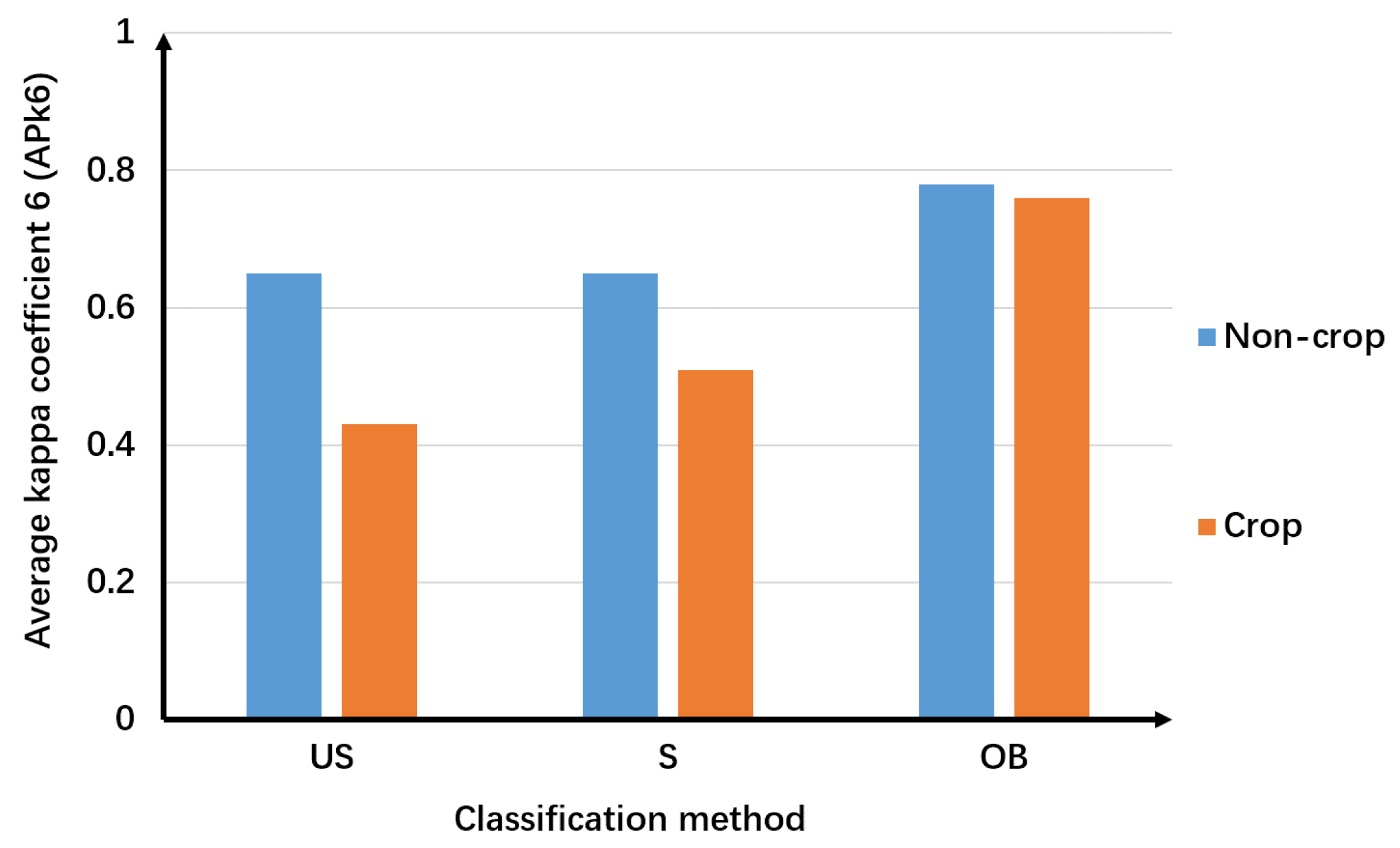
| AKp6 | 0.43 | 0.51 | 0.76 | |||||||
| (b) | Non-crop | Unsupervised | Supervised | Object-orient | ||||||
| 3US | 4US | AKp5 | 3S | 4S | AKp5 | 3OB | 4OB | AKp5 | ||
| IM | 0.79 | 0.90 | 0.85 | 0.66 | 0.68 | 0.67 | 0.92 | 0.92 | 0.92 | |
| BF | 0.71 | 0.71 | 0.71 | 0.77 | 0.71 | 0.74 | 0.72 | 0.79 | 0.76 | |
| GA | 0.38 | 0.28 | 0.33 | 0.44 | 0.46 | 0.45 | 0.51 | 0.59 | 0.55 | |
| FE | 0.50 | 0.39 | 0.45 | 0.45 | 0.60 | 0.53 | 0.89 | 0.85 | 0.87 | |
| WA | 0.88 | 0.92 | 0.90 | 0.80 | 0.92 | 0.86 | 0.71 | 0.88 | 0.80 | |
| AKp6 | 0.65 | 0.65 | 0.78 | |||||||
| Properties | Three-Band | Four-Band |
|---|---|---|
| Number of end nodes (number of branches) | 39 | 33 |
| Maximum number of tree levels | 10 | 10 |
| First level to use non-spectral features | 3 | 4 |
| Number of branches that used non-spectral features | 63 | 38 |
| Average times non-spectral features were used for each branch | 1.62 | 1.15 |
| Ratio of branches that used non-spectral features (%) | 95 | 82 |
© 2016 by the authors; licensee MDPI, Basel, Switzerland. This article is an open access article distributed under the terms and conditions of the Creative Commons by Attribution (CC-BY) license (http://creativecommons.org/licenses/by/4.0/).
Share and Cite
Zhang, J.; Yang, C.; Song, H.; Hoffmann, W.C.; Zhang, D.; Zhang, G. Evaluation of an Airborne Remote Sensing Platform Consisting of Two Consumer-Grade Cameras for Crop Identification. Remote Sens. 2016, 8, 257. https://0-doi-org.brum.beds.ac.uk/10.3390/rs8030257
Zhang J, Yang C, Song H, Hoffmann WC, Zhang D, Zhang G. Evaluation of an Airborne Remote Sensing Platform Consisting of Two Consumer-Grade Cameras for Crop Identification. Remote Sensing. 2016; 8(3):257. https://0-doi-org.brum.beds.ac.uk/10.3390/rs8030257
Chicago/Turabian StyleZhang, Jian, Chenghai Yang, Huaibo Song, Wesley Clint Hoffmann, Dongyan Zhang, and Guozhong Zhang. 2016. "Evaluation of an Airborne Remote Sensing Platform Consisting of Two Consumer-Grade Cameras for Crop Identification" Remote Sensing 8, no. 3: 257. https://0-doi-org.brum.beds.ac.uk/10.3390/rs8030257