
A 30+ Year AVHRR LAI and FAPAR Climate Data Record: Algorithm Description and Validation

Abstract
:
1. Introduction
2. Input Data
2.1. AVH09 Surface Reflectance
2.2. Reference LAI/FAPAR
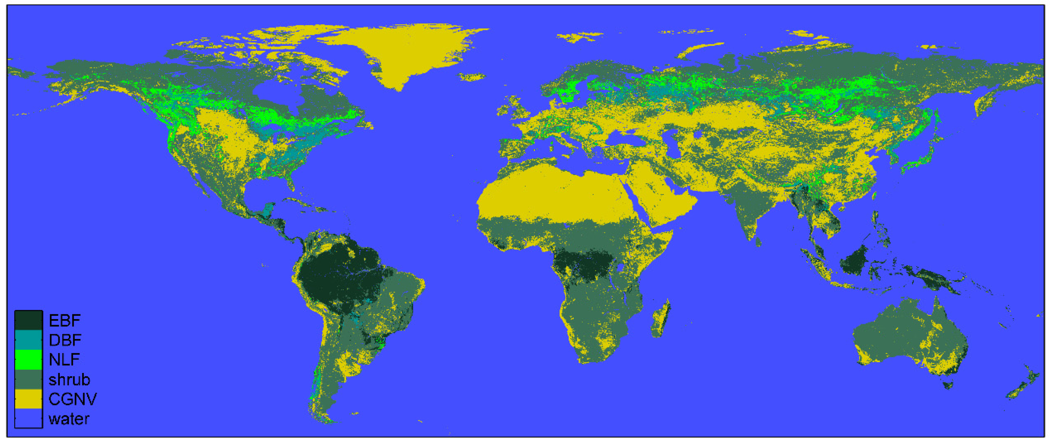
2.3. Land Cover Map
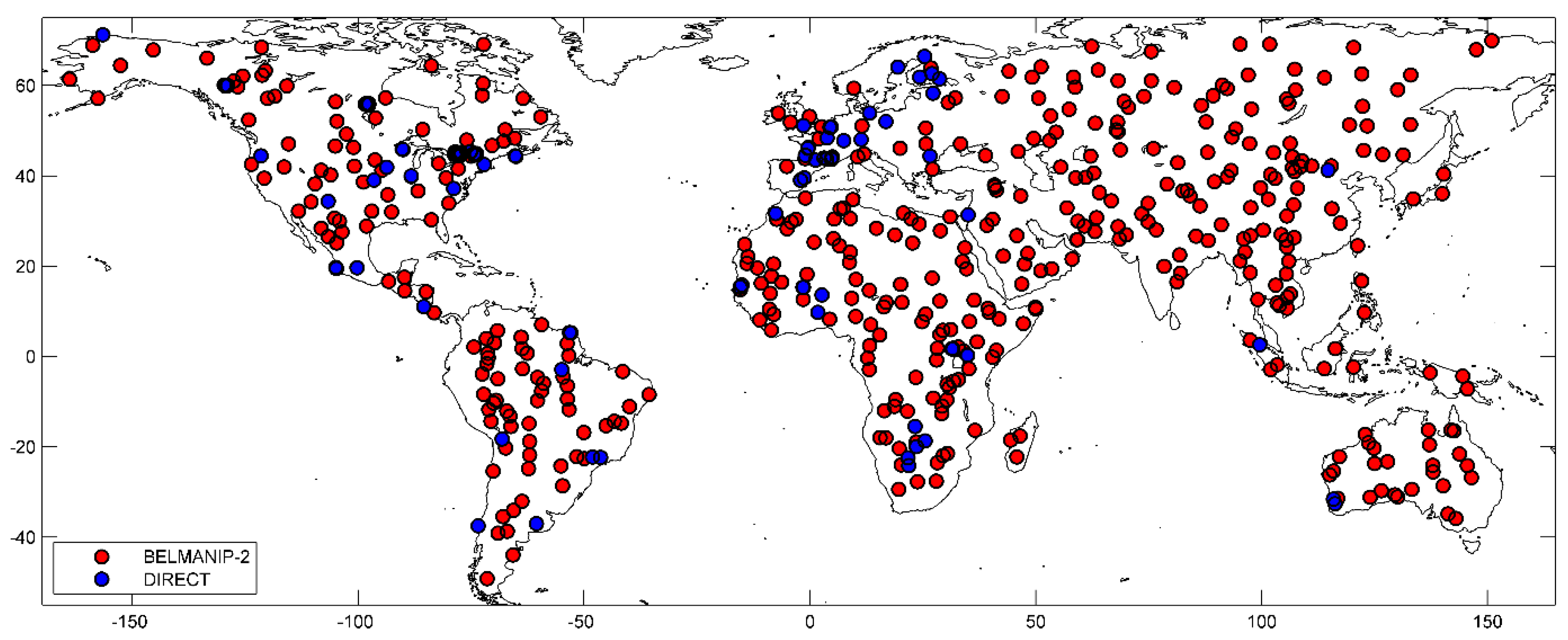
2.4. Calibration and Validation Sites
3. Algorithm Definition and Calibration
- -
- Input normalization,
- -
- ANN execution (per class and variable),
- -
- Output normalization,
- -
- Classes fusion according to the IGBP land cover as defined in Section 2.3, and
- -
- Flagging pixels outside of the defined domain.
3.1. Input and Output Normalization
3.2. ANN Definition and Learning
- -
- One input layer made of the four normalized inputs: AVH09 Red SR, AVH09 NIR SR, AVH13 NDVI and the cosine of the solar zenith angle,
- -
- One hidden layer with five neurons having hyperbolic tangent sigmoid transfer functions (Equation (3), where x is the neuron input and y the output),
- -
- One output layer via a linear transfer function, and
- -
- Normalized output.
3.3. Domain Definition
4. CDR Performance and Validation
5. Conclusions
Acknowledgments
Author Contributions
Conflicts of Interest
References
- Gobron, N.; Verstraete, M. Ecv t10 Fapar; GTOS: Rome, Italy, 2009. [Google Scholar]
- Gobron, N.; Verstraete, M. Ecv t11 Leaf Area Index (LAI); GTOS: Rome, Italy, 2009. [Google Scholar]
- GCOS. Systematic Observation Requirements for Satellite-Based Products for Climate (2011 Update); GCOS-154; GCOS: Geneva, Switzerland, 2011. [Google Scholar]
- Running, S.W.; Baldocchi, D.D.; Turner, D.P.; Gower, S.T.; Bakwin, P.S.; Hibbard, K.A. A global terrestrial monitoring network integrating tower fluxes, flask sampling, ecosystem modeling and EOS satellite data. Remote Sens. Environ. 1999, 70, 108–127. [Google Scholar] [CrossRef]
- Baret, F.; Hagolle, O.; Geiger, B.; Bicheron, P.; Miras, B.; Huc, M.; Berthelot, B.; Nino, F.; Weiss, M.; Samain, O.; et al. LAI, FAPAR and Fcover cyclopes global products derived from vegetation—Part 1: Principles of the algorithm. Remote Sens. Environ. 2007, 110, 275–286. [Google Scholar] [CrossRef] [Green Version]
- Claverie, M.; Vermote, E.F.; Weiss, M.; Baret, F.; Hagolle, O.; Demarez, V. Validation of coarse spatial resolution LAI and FAPAR time series over cropland in southwest france. Remote Sens. Environ. 2013, 139, 216–230. [Google Scholar] [CrossRef]
- Myneni, R.B.; Hoffman, S.; Knyazikhin, Y.; Privette, J.L.; Glassy, J.; Tian, Y.; Wang, Y.; Song, X.; Zhang, Y.; Smith, G.R.; et al. Global products of vegetation leaf area and fraction absorbed par from year one of MODIS data. Remote Sens. Environ. 2002, 83, 214–231. [Google Scholar] [CrossRef]
- Weiss, M.; Baret, F.; Garrigues, S.; Lacaze, R. Lai and fapar cyclopes global products derived from vegetation. Part 2: Validation and comparison with MODIS collection 4 products. Remote Sens. Environ. 2007, 110, 317–331. [Google Scholar]
- National Research Council. Climate Data Records from Environmental Satellites: Interim Report; The National Academies Press: Washington, DC, USA, 2004; p. 150. [Google Scholar]
- Vermote, E.; Justice, C.; Csiszar, I.; Eidenshink, J.; Myneni, R.; Baret, F.; Masuoka, E.; Wolfe, R.; Claverie, M.; Program, N.C. Noaa Climate Data Record (CDR) of Avhrr Surface Reflectance, version 4; NOAA National Climatic Data Center, Ed.; NOAA National Climatic Data Center: Asheville, NC, USA, 2014. [Google Scholar]
- Xiao, Z.; Liang, S.; Wang, J.; Chen, P.; Yin, X.; Zhang, L.; Song, J. Use of general regression neural networks for generating the glass leaf area index product from time-series MODIS surface reflectance. IEEE Trans. Geosci. Remote Sens. 2014, 52, 209–223. [Google Scholar] [CrossRef]
- Zhu, Z.; Bi, J.; Pan, Y.; Ganguly, S.; Anav, A.; Xu, L.; Samanta, A.; Piao, S.; Nemani, R.; Myneni, R. Global data sets of vegetation leaf area index (LAI)3g and fraction of photosynthetically active radiation (FPAR)3g derived from global inventory modeling and mapping studies (GIMMS) normalized difference vegetation index (ndvi3g) for the period 1981 to 2011. Remote Sens. 2013, 5, 927–948. [Google Scholar]
- Claverie, M.; Vermote, E.; Program, N.C. Noaa Climate Data Record (CDR) of Leaf Area Index (LAI) and Fraction of Absorbed Photosynthetically Active Radiation (FAPAR), version 4; NOAA National Climatic Data Center, Ed.; NOAA National Climatic Data Center: Asheville, NC, USA, 2014. [Google Scholar]
- Vermote, E.; Justice, C.O.; Breon, F.-M. Towards a generalized approach for correction of the BRDF effect in MODIS directional reflectances. IEEE Trans. Geosci. Remote Sens. 2009, 47. [Google Scholar] [CrossRef]
- Vermote, E.; Claverie, M. Avhrr Land Bundle - Surface Reflectance and Normalized Difference Vegetation Index: Climate Algorithm Theoretical Basis Document; NOAA National Climatic Data Center: Asheville, NC, USA, 2013. [Google Scholar]
- Roujean, J.-L.; Leroy, M.; Deschamps, P.Y. A bidirectional reflectance model of the earth's surface for the correction of remote sensig data. J. Geophys. Res. 1992, 97, 20455–20468. [Google Scholar] [CrossRef]
- Li, X.W.; Strahler, A.H. Geometric-optical bidirectional reflectance modeling of the discrete crown vegetation canopy: Effect of crown shape and mutual shadowing. IEEE Trans. Geosci. Remote Sens. 1992, 30, 276–292. [Google Scholar] [CrossRef]
- Knyazikhin, Y.; Martonchik, J.V.; Myneni, R.B.; Diner, D.J.; Running, S.W. Synergistic algoritm for estimating vegetation canopy leaf area index and fraction of absorbed photosynthetically active radiation from MODIS and MISR data. Geophys. Res. 1998, 103, 32257–32276. [Google Scholar] [CrossRef]
- Vermote, E.F.; Tanre, D.; Deuze, J.L.; Herman, M.; Morcrette, J.J. Second simulation of the satellite signal in the solar spectrum, 6S: An overview. IEEE Trans. Geosci. Remote Sens. 1997, 35, 675–686. [Google Scholar] [CrossRef]
- Yang, W.; Tan, B.; Huang, D.; Rautiainen, M.; Shabanov, N.; Wang, Y.; Privette, J.; Huemmrich, K.; Fensholt, R.; Sandholt, I.; et al. MODIS leaf area index products: From validation to algorithm improvement. IEEE Trans. Geosci. Remote Sens. 2006, 44, 1885–1898. [Google Scholar] [CrossRef]
- Hansen, M.; DeFries, R.; Townshend, J.R.G.; Sohlberg, R. Umd Global Land Cover Classification, 1 Kilometer, 1981–1994, 1.0; Department of Geography, University of Maryland: College Park, MD, USA, 1998. [Google Scholar]
- Baret, F.; Morissette, J.; Fernandes, R.; Champeaux, J.; Myneni, R.; Chen, J.; Plummer, S.; Weiss, M.; Bacour, C.; Garrigues, S.; et al. Evaluation of the representativeness of networks of sites for the global validation and intercomparison of land biophysical products: Proposition of the CEOS-BELMANIP. IEEE Trans. Geosci. Remote Sens. 2006, 44, 1794–1803. [Google Scholar] [CrossRef]
- Garrigues, S.; Lacaze, R.; Baret, F.; Morisette, J.T.; Weiss, M.; Nickeson, J.E.; Fernandes, R.; Plummer, S.; Shabanov, N.V.; Myneni, R.B.; et al. Validation and intercomparison of global leaf area index products derived from remote sensing data. J. Geophys. Res.-Biogeosci. 2008, 113, G2. [Google Scholar] [CrossRef]
- Weiss, M.; Baret, F.; Block, T.; Koetz, B.; Burini, A.; Scholze, B.; Lecharpentier, P.; Brockmann, C.; Fernandes, R.; Plummer, S.; et al. On line validation exercise (olive): A web based service for the validation of medium resolution land products. Application to fapar products. Remote Sens. 2014, 6, 4190–4216. [Google Scholar] [CrossRef]
- Demuth, H.; Beale, M. Neural Network Toolbox for Use with Matlab; The MathWorks Inc.: Natick, MA, USA, 1998. [Google Scholar]
- Moré, J. The levenberg-marquardt algorithm: Implementation and theory. In Numerical Analysis; Watson, G.A., Ed.; Springer: Berlin, Germany; Heidelberg, Germany, 1978; Volume 630, pp. 105–116. [Google Scholar]
- Douglas, D.H.; Peucker, T.K. Algorithms for the reduction of the number of points required to represent a digitized line or its caricature. In Classics in Cartography; John Wiley & Sons, Ltd.: Hoboken, NJ, USA, 2011; pp. 15–28. [Google Scholar]
- Vermote, E.F.; Kotchenova, S. Atmospheric correction for the monitoring of land surfaces. J. Geophys. Res.-Atmos. 2008, 113, D23. [Google Scholar] [CrossRef]
- Weiss, M.; Baret, F.; Smith, G.J.; Jonckheere, I.; Coppin, P. Review of methods for in situ leaf area index (LAI) determination. Part II. Estimation of LAI, errors and sampling. Agric. For. Meteorol. 2004, 121, 37–53. [Google Scholar] [CrossRef]
- Roman, M.O.; Gatebe, C.K.; Shuai, Y.; Wang, Z.; Gao, F.; Masek, J.G.; He, T.; Liang, S.; Schaaf, C.B. Use of in situ and airborne multiangle data to assess MODIS-and Landsat-based estimates of directional reflectance and albedo. IEEE Trans. Geosci. Remote Sens. 2013, 51, 1393–1404. [Google Scholar] [CrossRef]
- Claverie, M. Estimation spatialisée de la biomasse et des besoins en eau des cultures à l’aide de données satellitales à hautes résolutions spatiale et temporelle: Application aux agrosystèmes du sud-ouest de la france. Toulouse 3, 2012. [Google Scholar]
- Camacho, F.; Cemicharo, J.; Lacaze, R.; Baret, F.; Weiss, M. Geov1: LAI, FAPAR essential climate variables and FCOVER global time series capitalizing over existing products. Part 2: Validation and intercomparison with reference products. Remote Sens. Environ. 2013, 137, 310–329. [Google Scholar] [CrossRef]


| Short Name | New Class Name | Original IGBP Class Name |
|---|---|---|
| NLF | Needle leaf forest | Needle leaf forest |
| DBF | Deciduous broadleaf forest | Deciduous broadleaf forest, mixed forests |
| Shrub | Shrubland | Closed/open/woody shrubland, savannas |
| CGNV | Croplands & grasslands & non-vegetated | Grasslands, permanent wetlands, croplands, urban and built-up, cropland/natural vegetation mosaic, snow and ice, barren or sparsely vegetated |
| EBF | Evergreen broadleaf forest | Evergreen broadleaf forest |
| water | Water | Water |
| Class | EBF | DBF | NLF | Shrub | CGNV | |||||
|---|---|---|---|---|---|---|---|---|---|---|
| Min | Max | Min | Max | Min | Max | Min | Max | Min | Max | |
| Red | 0.01 | 0.31 | 0.01 | 0.12 | 0.01 | 0.11 | 0.01 | 0.29 | 0.02 | 0.42 |
| NIR | 0.01 | 0.37 | 0.04 | 0.39 | 0.02 | 0.24 | 0.01 | 0.39 | 0.02 | 0.48 |
| cos(ϴs) | 0.46 | 0.88 | 0.14 | 0.88 | 0.05 | 0.85 | 0.06 | 0.88 | 0.01 | 0.88 |
| NDVI | −0.41 | 0.91 | −0.01 | 0.87 | 0.01 | 0.86 | −0.22 | 0.92 | −0.22 | 0.80 |
| LAI | 0.69 | 6.72 | 0.01 | 5.94 | 0.00 | 5.24 | 0.00 | 5.95 | 0.00 | 5.27 |
| FAPAR | 0.23 | 0.91 | 0.02 | 0.92 | 0.01 | 0.93 | 0.00 | 0.89 | 0.00 | 0.89 |
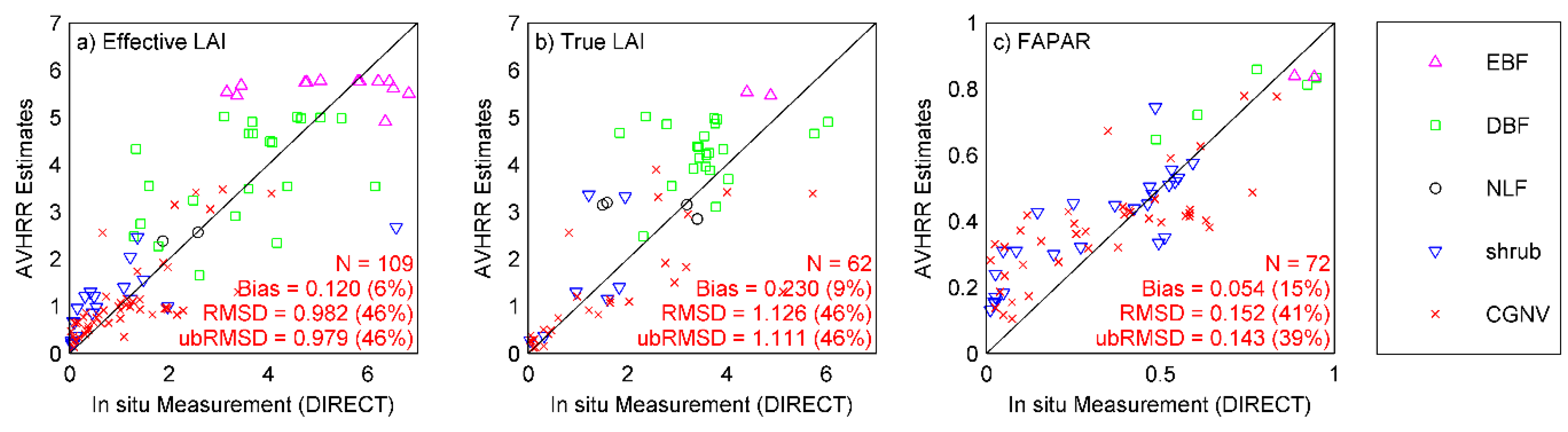
| Class | Effective LAI | True LAI | FAPAR | |||||||||
|---|---|---|---|---|---|---|---|---|---|---|---|---|
| Bias | ubRMSD | RMSD | N | Bias | ubRMSD | RMSD | N | Bias | ubRMSD | RMSD | N | |
| EBF | 0.24 | 1.33 | 1.31 | 14 | 0.85 | 0.39 | 0.90 | 2 | −0.08 | 0.04 | 0.08 | 2 |
| DBF | 0.36 | 1.27 | 1.29 | 22 | 0.68 | 1.01 | 1.20 | 22 | 0.03 | 0.13 | 0.12 | 5 |
| NLF | 0.25 | 0.37 | 0.36 | 2 | 0.66 | 1.13 | 1.18 | 4 | N/A | N/A | N/A | 0 |
| Shrub | 0.18 | 1.06 | 1.05 | 20 | 0.46 | 0.96 | 1.00 | 7 | 0.08 | 0.12 | 0.14 | 25 |
| CGNV | −0.04 | 0.67 | 0.66 | 51 | −0.31 | 1.08 | 1.10 | 27 | 0.05 | 0.16 | 0.16 | 40 |
| All | 0.12 | 0.98 | 0.98 | 109 | 0.23 | 1.11 | 1.13 | 62 | 0.05 | 0.14 | 0.15 | 72 |
© 2016 by the authors; licensee MDPI, Basel, Switzerland. This article is an open access article distributed under the terms and conditions of the Creative Commons by Attribution (CC-BY) license (http://creativecommons.org/licenses/by/4.0/).
Share and Cite
Claverie, M.; Matthews, J.L.; Vermote, E.F.; Justice, C.O. A 30+ Year AVHRR LAI and FAPAR Climate Data Record: Algorithm Description and Validation. Remote Sens. 2016, 8, 263. https://0-doi-org.brum.beds.ac.uk/10.3390/rs8030263
Claverie M, Matthews JL, Vermote EF, Justice CO. A 30+ Year AVHRR LAI and FAPAR Climate Data Record: Algorithm Description and Validation. Remote Sensing. 2016; 8(3):263. https://0-doi-org.brum.beds.ac.uk/10.3390/rs8030263
Chicago/Turabian StyleClaverie, Martin, Jessica L. Matthews, Eric F. Vermote, and Christopher O. Justice. 2016. "A 30+ Year AVHRR LAI and FAPAR Climate Data Record: Algorithm Description and Validation" Remote Sensing 8, no. 3: 263. https://0-doi-org.brum.beds.ac.uk/10.3390/rs8030263