Article

Pi-SAR-L2 Observation of the Landslide Caused by Typhoon Wipha on Izu Oshima Island

by
Manabu Watanabe
1,*,
Rajesh Bahadur Thapa
1 and
Masanobu Shimada
1,2
1
Earth Observation Research Center, Japan Aerospace Exploration Agency, 2-1-1 Sengen, Tsukuba, Ibaraki 305-8505, Japan
2
Tokyo Denki University, Ishizaka, Hatoyama-machi, Hiki-gun, Saitama 350-0394, Japan
*
Author to whom correspondence should be addressed.
Submission received: 24 December 2015 / Revised: 16 March 2016 / Accepted: 22 March 2016 / Published: 29 March 2016
(This article belongs to the Special Issue Earth Observations for Geohazards)

Abstract

:
Pi-SAR-L2 full polarimetic data observed in four different observational directions over a landslide area on Izu Oshima Island, induced by Typhoon Wipha on 16 October 2013, were analyzed to clarify the most appropriate L-band full polarimetric parameters and observational direction to detect a landslide area. Japanese airborne Pi-SAR-L2 and PiSAR-L data were used in this analysis. Several L-band full polarimetric parameters, including backscattering coefficient (σ°), coherence between two polarimetric states, four-component decomposition parameters (double-bounce/volume/surface/helix scattering), and eigenvalue decomposition parameters (entropy/α/anisotropy), were calculated to determine the most appropriate parameters for detecting landslide areas. The change in land cover from forest before the disaster to bare soil after the disaster was detected well by α, and coherence between HH and VV. Observational data from the bottom to the top of the landslide detected the landslide well, whereas observations from the opposite sides were not as useful, indicating that a smaller local incident angle is better to distinguish landslide and forested areas. Soil from the landslide intruded into the urban areas; however, none of the full polarimetric parameters showed any significant differences between the landslide-affected urban areas after the disaster and unaffected areas before the disaster.

Graphical Abstract

1. Introduction

Full polarimetric SAR data are capable of identifying radar scattering mechanisms on the ground, and they have been used to estimate land cover class by connecting the radar backscattering mechanism to the land cover condition both by day and by night in all weather conditions. Such characteristics make these data applicable to the detection of a disaster area, especially for emergency observations made soon after a disaster happens. Watanabe et al. [1] used Japanese L-band satellite SAR (PALSAR; Phased Array type L-band Synthetic Aperture Radar) full polarimetric data to detect landslide areas induced by the Iwate-Miyagi Nairuku earthquake of 2008, using the surface scattering component of a three-component decomposition model. Furthermore, σ°HV has also been used to distinguish landslide areas with rough surfaces from other surface scattering areas, such as pastures and vacant pieces of land with smooth surfaces.
Polarimetric decomposition analysis was conducted on the data before and after a landslide event with ALOS PALSAR data [2]. For the detection of landslides areas, 30-m resolution full polarimetric data using unsupervised classification based on the Entropy plane are more useful than 10-m resolution single-polarization data. Czuchlewski et al. [3] use L-band airborne SAR polarimetry data, and identify the extent of the landslide, using scattering entropy, anisotropy, and pedestal height. They also pointed out that one post-event single polarized SAR image is insufficient for distinguishing and mapping landslides. Rodriguez et al. [4] use L-band airborne SAR polarimetry data, and show the landslide scar areas are dominated by single-bounce scattering and the surrounding forested regions are dominated by volume scattering. Radar vegetation index, pedestal height, and entropy are used to identify forest, to separate the landslide area. Shimada et al. [5] used Japanese L-band airborne SAR (Pi-SAR-L2; Polarimetric and Interferometric Airborne Synthetic Aperture Radar L2) data to show that the change of land cover from forest before a disaster to bare soil after a disaster was detected well by the polarimetric coherence between HH and VV (γ(HH)-(VV)). Shibayama et al. [6] confirm the usefulness of γ(HH)-(VV) for detecting a landslide. They also pointed out that in landslide areas, the polarimetric indices of normalized surface scattering power (ps), normalized volume scattering power (pv), and γ(HH)-(VV) change drastically with the local incidence angle, whereas in forested areas, these indices are stable, regardless of the change in the local incidence angle. Several full polarimetric parameters have been suggested to detect a landslide area since now. In this study, airborne full polarimetric L-band SAR data, obtained both before and after a landslide event, were used to determine the most appropriate full polarimetric parameters and observation direction for identifying an area affected by a landslide induced by heavy rain. The data used in our analysis are unique for two reasons:
(1)
hey comprise full polarimetric data observed just after the disaster (landslide).
(2)
They were observed from four different observational directions at the same time after the disaster. One of the directions was also observed before the disaster.
To generalize our method, simple radar scattering models from rough surface were applied, as discussed in Section 4. The models were evaluated for two sites using three different local incident angles with two polarizations, simultaneously, which has rarely been undertaken for a landslide area.

2. Pi-SAR-L2 Data and Field Experiment

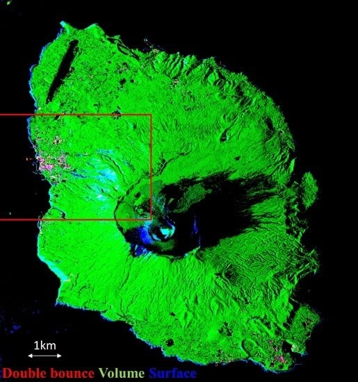
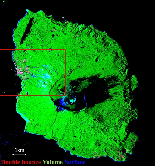
On 16 October 2013, Typhoon Wipha struck Izu Oshima Island, which is located 100 km south of Tokyo (Figure 1), generating a rainfall rate that was recorded at 122.5 mm/h. This heavy rain induced a large-scale landslide that affected an area of 1.14 million m2 and led to 39 people being killed or missing. The Geospatial Information Authority of Japan (GSI) used aerial photographs taken after the disaster to produce a landslide map [7], and the main landslide areas are identified in Figure 2. The locations of many landslides can be observed in the mountain area, and some material displaced by the landslides intruded into residential areas. These data were used as the validation data.
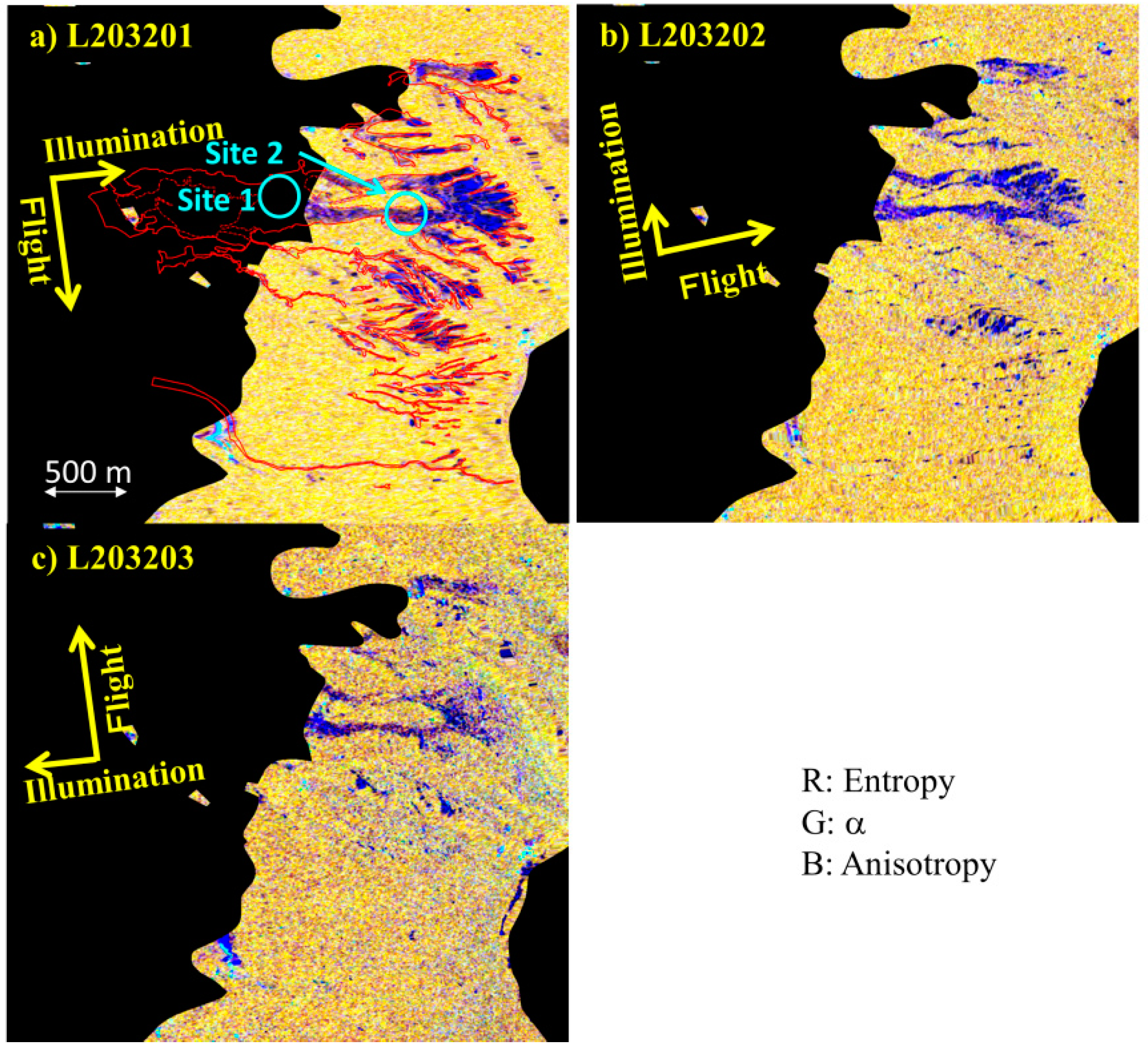
The study area was observed before and after the disaster using Japanese airborne SAR (Pi-SAR-L and Pi-SAR-L2) (Table 1). The Pi-SAR-L2 observations were acquired in four different observational directions (L203201–L203204, Figure 1) six days after the disaster. The time required for the four flights was about one hour. Before the disaster, one Pi-SAR-L observation (L03801) had been made on 30 August 2000, in the same observational direction as L203201. Three of the four data (L203201, L203202, and L203203) were used to determine the parameters and directions most appropriate for detecting landslide areas. L203204 was not used, because its configuration (incident and azimuth angles to the landslide area) is almost same as L203202 data. These parameters for detecting landslide areas included backscattering coefficient (σ°), polarimetric coherence (γ), eigenvalue decomposition [8], and four-component decomposition parameters [9]. The γ is calculated from the correlation between two polarimetric states (HH-HV-VV base, (HH+VV)-(HH-VV)-(HV) base). The eigenvalue decomposition parameters consist of entropy/α/anisotropy, and they were obtained using PolSARPro [
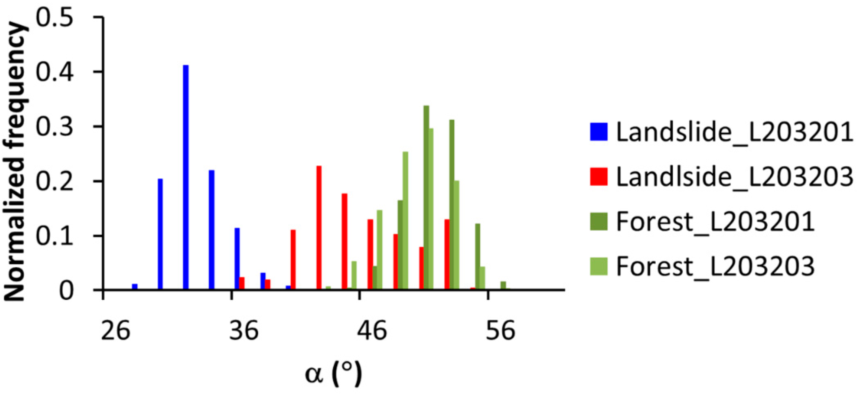
10]. Entropy represents the randomness of a scatterer, α represents the scattering mechanism (0° for surface scattering, 45° for dipole scattering or single scattering by a cloud of anisotropic particles, and 90° for double-bounce scattering), and anisotropy represents the relative importance of the second and the third eigenvalues. The four-component decomposition parameters (double-bounce/volume/surface/helix scattering) are related to surface, volume, double-bounce, and helix scattering components on the earth’s surface, and they were obtained using a program of our own making. The processing window size for calculating the parameters was 7 × 7 pixels.
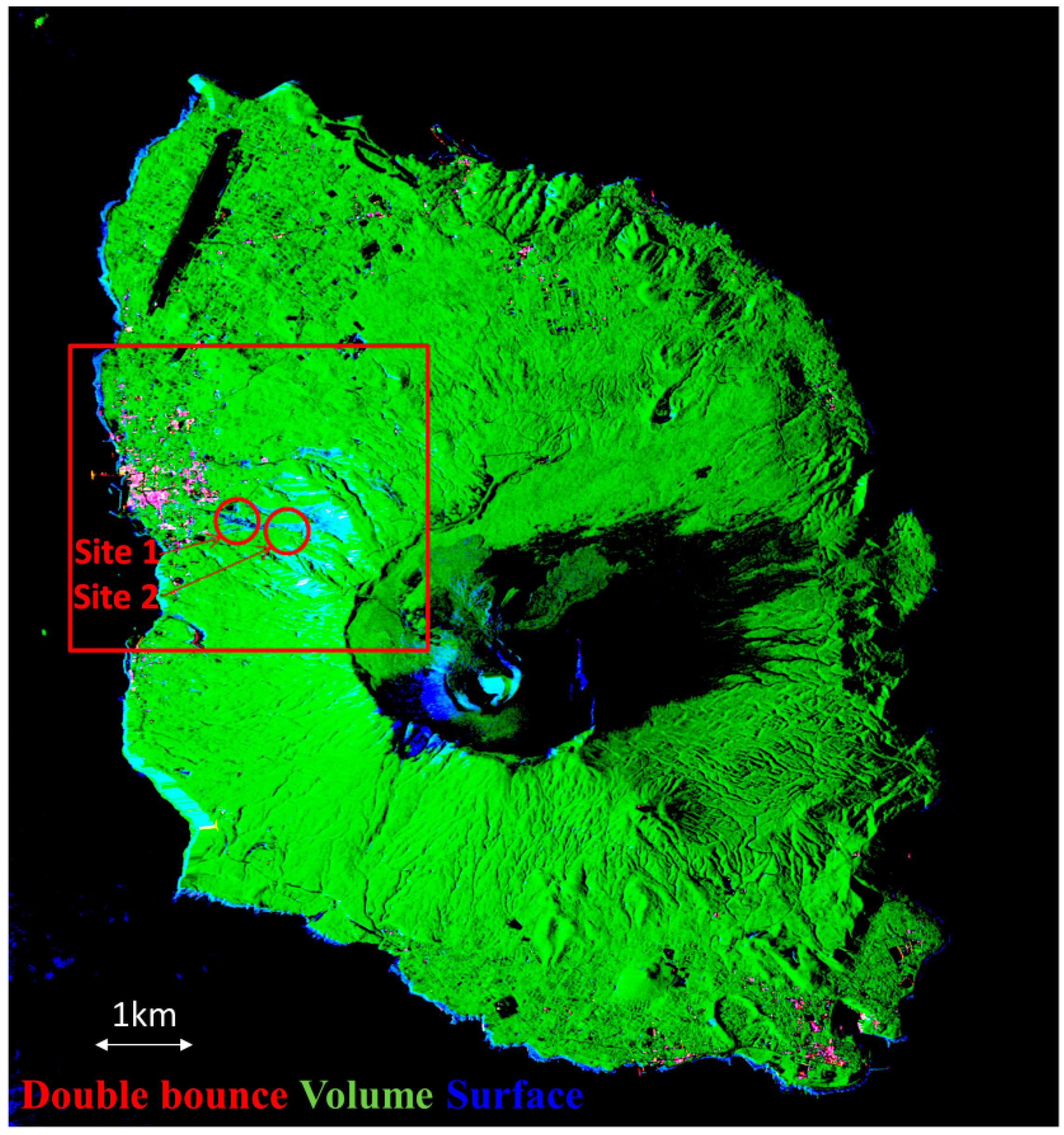
A forest area map, obtained from the national land numerical information download service managed by GSI (Figure 2), was used to identify the forest area before the disaster [11]. Field experiments were performed on 23 and 24 March 2015. The value of σ° obtained from bare soil is determined from the surface roughness, dielectric constant of the soil (equivalent to the volumetric soil moisture, Mv), and local incident angle. The parameter Mv was not measured in the field experiments because its value was different from that when the Pi-SAR-L2 observation was performed. However, surface roughness does not change much, if there is no disturbance. It was measured using a needle profiler at two sites (Sites 1 and 2, Figure 2) within the landslide area to evaluate the radar backscattering from bare soil (Figure 3). The red points shown in the photos were used to evaluate the surface roughness (s) and correlation length (l) normalized by wave number k (e.g., ks and kl). Site 1 was a slightly rough surface covered by soil with a slope of 5°, for which ks and kl were evaluated as 0.38 and 6.17, respectively. Site 2 was a rough surface covered by soil and volcanic rocks with a slope of 20°, for which the values of ks and kl were determined as 1.85 and 5.03, respectively.
There are three well known and simple surface scattering models. The first of these is the small perturbation model (SPM) [12], which is valid for smooth surfaces (ks < 0.3). The second, the physical optics model (POM) [13], is valid for slightly rough surfaces within the parameter ranges Mv < 0.25, l2 > 2.76·sλ, and kl > 6. The third, the geometric optics model (GOM) [13], is valid for rough surfaces and predicts that σ°HH = σ°VV at all incidence angles; this model is valid within the parameter ranges kl > 6, l2 > 2.76·sλ, and ks·cosθ > 1.5. The POM [13] is valid for Site 1, and is described by:
σ 0 p p ( θ ) = k 2 cos 2 θ Γ p ( θ ) exp [ ( 2 ks cos θ ) 2 ] n = 1 ( 2 ks cos θ ) 2 n n ! I
I exponential = nl 2 [ n 2 + 2 ( kl sin θ ) 2 ] 3 / 2
In these equations, Γ(θ,ε) represents the Fresnel reflection coefficient, p represents the polarization (h or v), pp represents any combination of h and v, such as hh, hv, vh, vv, l is the correlation length, θ is the local incident angle, and ε is the relative dielectric constant, which is related to the soil moisture. The GOM [13] is almost valid for Site 2, and described by:
σ 0 p p ( θ ) = Γ ( 0 ) exp 2 ( tan 2 θ / 2 m 2 ) 2 m 2 cos 4 θ
Γ ( 0 ) = 1 ε 1 + ε
where m is the surface slope and represented by 2 s / l .
These models and parameters obtained in the field experiment were used to evaluate the observed σ° in Section 4.

3. Results

3.1. Landslide Area Detection with Full Polarimetric Parameters

The four-component decomposition image obtained by Pi-SAR-L2 (ID: L203201) is presented in Figure 4. Maximum and minimum digital number values for each four-component decomposition parameter were assigned to values of 0 and 255 in the RGB scale. The actual landslide is represented by the blue color, indicating that surface scattering is dominant. However, similar surface scattering can also be observed near the top of Mt. Mihara, the volcanic mountain located in the center of the island. The same situation was also observed for the other parameters (entropy, α, polarimetric coherence between (HH+VV) and (HH−VV) (γ(HH+VV)-(HH−VV)), γHH-VV), and two of the representative parameters, γ(HH+VV)-(HH−VV), and α are shown in Figure 5a,c.
The differences in these parameters before and after the disaster (Δγ(HH+VV)-(HH−VV), Δα) can be established by visual inspection (Figure 5b,d). It can be seen that the Δγ(HH+VV)-(HH−VV) shows differences for both the landslide area and the top of the mountain, where no landslide occurred, whereas Δα shows differences in the landslide area only. This indicates that α is better than γ(HH+VV)-(HH−VV) for detecting landslide areas in large scale images. Two other parameters (Δγ(HH)-(VV) and Δentropy) also showed the same characteristics as Δα; however, four-component decomposition parameters (Δσ°Double, Δσ°Volume, Δσ°Surface, Δσ°Helix in digital numbers), Δσ° (in digital number, and Δanisotropy, showed differences not only for the landslide area, but also the bare soil area, where no landslide occurred. The visual interpretation revealed that entropy, α, and γHH-VV were the prospective parameters for the detection of landslide areas from large scale images.
The user’s and producer’s accuracies (Story and Congalton, [14]) for entropy, α, and γHH-VV were evaluated from the error matrices to estimate the classification accuracy for detecting the landslide areas shown in the red rectangle in Figure 5. Threshold levels were estimated from a cross-over point obtained from the histogram of the landslide and non-landslide areas for each parameter. The classification was conducted based on the threshold level. Two classes (landslide and no landslide) have been set, and classification accuracy for the case using parameters obtained after the disaster, and the case using the difference in the parameter values before and after the disaster are evaluated. The results are summarized in Table 2. User accuracy is a measure indicating the probability that a pixel is grouped into Class A, given that the classifier has labeled the pixel as belonging to Class A. The producer accuracy is a measure indicating the probability that the classifier has labeled an image pixel as belonging to Class A, given that the ground truth is Class A. The accuracies for γ(HH+VV)-(HH−VV) are also shown in the same table for reference. When the data before and after the disaster were used, the values of Δα and ΔγHH-VV show user’s accuracies of about 58.7%–60.9% and producer’s accuracies of about 33.8%–35.8%. The producer’s accuracies are better than those of 25.9%–26.8% for Δentropy and Δγ(HH+VV)-(HH−VV). The accuracies are almost the same as those achieved when using parameters obtained after the disaster, i.e., the values of α and γHH-VV show user’s accuracies of about 59.5%–61.8% and producer’s accuracies of about 34.0%–38.4%. The producer’s accuracies of about 11.7%–11.8% for entropy and γ(HH+VV)-(HH−VV) obtained after the disaster are 14.2%–15% lower than Δentropy and Δγ(HH+VV)-(HH−VV). This may be due to the poor classification accuracy between a forest and landslide areas in these parameters.
The landslide area detection was performed for the forest area before the landslide using the forest map and the results are also presented in Table 2. Producer’s accuracies are especially improved, and the accuracy changes from 35.8% to 52.2% for the α parameter (improved by 16.4%), and from 33.8% to 49.5% for the γ(HH)-(VV) parameters (improved by 15.7%).

3.2. Landslide Area Detection in Three Different Observational Directions

The entropy, α, and anisotropy obtained from the three different observational directions (L203201, L203202, and L203203) with the forest mask, where only the forest area is picked up, are presented in Figure 6. The main landslide area is delineated by the red rectangle. The forest area is indicated as the yellow area and the blue area represents the bare soil area, which also indicates the landslide area. A visual inspection reveals that the landslide area is detected well in L203201, wherein observations are made from the bottom to the top of the landslide, whereas the clarity is lower in L203203, with observations made from the top to the bottom of the landslide.
The α and γ(HH)-(VV) values derived from L203201 and L203203 are presented in Table 3 for Site 1, Site 2, and a forest near Site 2. The values obtained from L203202 lie between those for L203201 and L203203 and have been omitted from the table. Small directional dependency can be observed for Site 1, because the slope is 5°. Small directional dependency is also observed for the forest area near Site 2, because random scattering in the forest canopy induces less directional dependency. However, relatively larger directional dependency can be observed for Site 2, because the slope is 20°.
Histograms of α for Site 2 and the forest near Site 2 are compared to examine the detectability of the landslide area in a forested region; the results are presented in Figure 7. The histograms for the forested area shows same for L203201 and L203203, indicating there is no local incident angle dependency. On the other hand, the histograms for the landslide area shows difference, indicating the local incident angle dependency. The results are consistent with the one obtained by Shibayama et al. [6]. The α value from landslide area in L203201 is clearly different from the value obtained from the forest, whereas the α value from landslide area in L203203 overlaps that from the forest. Some of the landslide area is misclassified as forest, which reduces the classification accuracy in L203203. The same pattern is observed for the γ(HH)-(VV) case. This indicates that a smaller local incident angle is better to distinguish landslide and forested areas.
The user’s and producer’s accuracies for detecting the landslide areas based on the different observational directions by α are summarized in Table 4. L203201 shows good accuracy with user’s and producer’s accuracies of 66.7% and 52.1%, respectively. L203203 shows the worst accuracy with user’s and producer’s accuracies of 59.1% and 16.4%, respectively, as was expected from the visual inspection in Figure 6.

4. Discussion

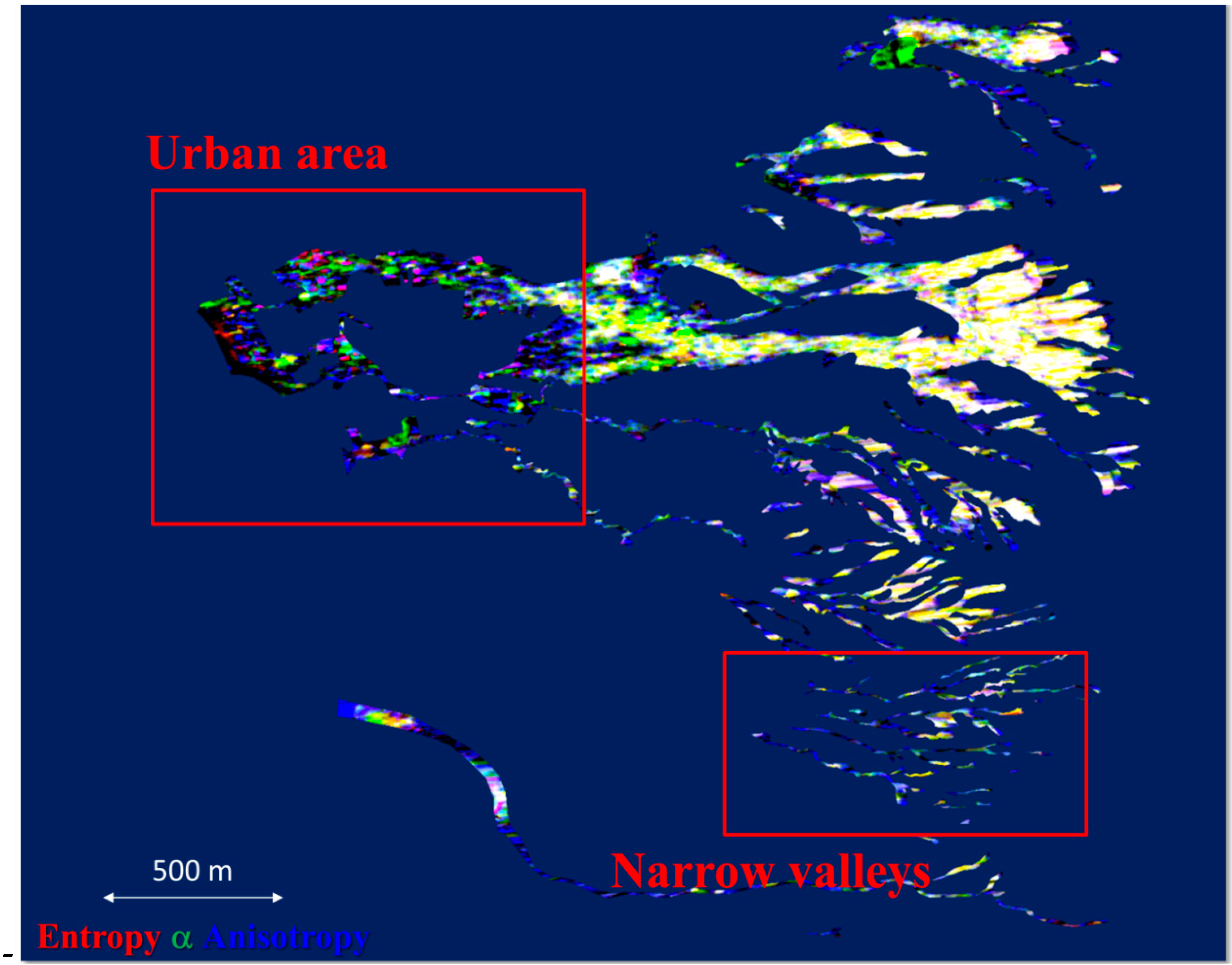
The accuracy of detection of the landslide area was improved when the forest area was picked up. The landslide area is picked up and shows the difference of entropy/α/anisotropy only before and after the disaster in Figure 8. Maximum and minimum values for each parameter are assigned to values of 0 and 255 in the RGB scale. Yellow areas seen in the upper right of Figure 8 indicate the significant change in entropy and α before and after the disaster. To a large extent, this area changed from forest to bare soil after the landslide. However, significant parameter change is not observed in the upper-left area of Figure 8. This is the residential area, which changed from a normal residential area before the disaster to a residential area with mud induced by the landslide after the disaster. No significant change could be detected by the full polarimetric parameters in this area. There are other areas without significant parameter change, such as in the lower right of Figure 8. Here, there are many narrow valleys and layover/shadowing might prevent any significant change in the full polarimetric parameters in this region. An outline of the detection accuracy by using ΔγHH-VV and Δα is presented in Figure 9. The misidentification of the residential area and the narrow valleys result in a low producer’s accuracy of 33.8%–35.8%. On the other hand, the higher user’s accuracy of 58.7%–60.9% is due to the detection of the change from forested area to landslide area.
γ(HH+VV)-(HH−VV) for the landslide area is lower than γ(HH)-(VV) (Table 3). Very little double-bounce scattering, indicated by HH−VV component, is expected from the landslide area, and this led to the smaller γ(HH+VV)-(HH−VV). Since a smaller γ(HH+VV)-(HH−VV) indicates a smaller Δγ(HH+VV)-(HH−VV) between the landslide and forested area, detection accuracy for the γ(HH+VV)-(HH−VV) parameter is lower than that for the γ(HH)-(VV) parameter. The γ(HH+VV)-(HH−VV) parameter highlights changes at the top of Mt. Mihara (Figure 5b). Small changes in vegetation and soil moisture are expected between the August and October observations; γ(HH+VV)-(HH−VV) may be sensitive to such changes, unlike γ(HH)-(VV) and α.
The accuracy is almost the same when using α and γ(HH)-(VV) after the disaster, and using the difference between α and γ(HH)-(VV) before and after the disaster. This indicates that α and γ(HH)-(VV) are good parameters to distinguish forest and bare soil areas. This is also supported by the accuracy improvement after the forest area is identified. The α and γ(HH)-(VV) obtained before the disaster are essential for distinguishing between areas of bare soil before the disaster and landslides induced by the disaster, and between bare soil and forest.
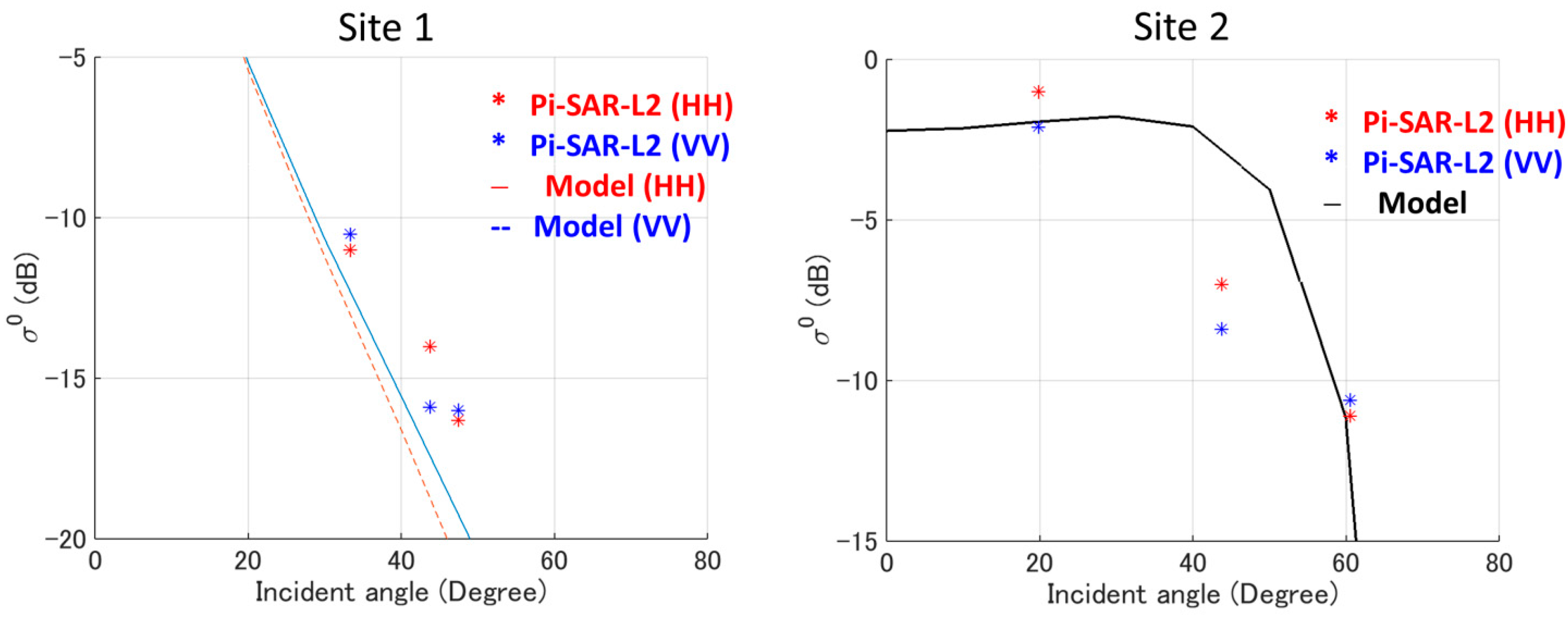
The values of σ° obtained from Pi-SAR-L2 and estimated from theoretical models are plotted against the local incident angle in Figure 10. The L203201, L203202, and L203203 observations correspond to the minimum, median, and maximum local incident angle plots in the figure. Pi-SAR-L2 observations were performed six days after the disaster, and the value of Mv is assumed as 100% for Site 1. The values of σ° obtained from Pi-SAR-L2 show the same pattern against the local incident angle, but with an offset of a few dB from the POM. If the value of ks was not 0.38 (measured on site), it was assumed as 0.5, and the model describes the data obtained from the three different local incident angles well. There was a 1.5-year interval between the Pi-SAR-L2 observations and surface roughness measurements and, thus, changes of 30% in the smoothness of the surface during that period could account for the difference of a few dB in the σ° values. The GOM works well for Site 2 if Mv = 25% is assumed, except for the L203202 data. The dielectric constant of volcanic rock, which partly covers the surface of Site 2, is generally 5–10, and this corresponds to an Mv of 8%–18.8%. The assumption of Mv = 25% could be explained by the mixture of the rock and soil. At Site 2, a few larger rocks could not be characterized by the surface roughness measurements and the shadowing of these rocks might unexpectedly have affected the values of σ° for the L203202 observations. However, the values of σ° observed for the landslide areas are represented moderately by the simple surface scattering models.

5. Conclusions

Pi-SAR-L2 full polarimetric data observed in four different observational directions over a landslide area were analyzed to clarify the most appropriate L-band full polarimetric parameters and observational direction to detect a landslide area. Data from one Pi-SAR-L observation performed before the disaster occurred were also used in this analysis. A summary of the preferable parameters to detect the landslide area was added in Table 5.
When the data before and after the disaster were used, the Δα and ΔγHH-VV showed user’s accuracies of about 58.7%–60.9% and producer’s accuracies of 33.8%–35.8%, indicating better performance than the other parameters, such as the four-component decomposition parameters (Δσ°Double, Δσ°Volume, Δσ°Surface, and Δσ°Helix), Δσ°, Δγ(HH+VV)-(HH−VV), Δentropy, and Δanisotropy.
Other two knowledge obtained from our analysis are:
The detection accuracy is almost the same when using the parameters after the disaster, and using the difference between the parameters before and after the disaster.
Producer’s accuracies are improved, and the accuracy changes from 35.8% to 52.2% for the α parameter (improved by 16.4%), and from 33.8% to 49.5% for the γ(HH)-(VV) parameters (improved by 15.7%), when evaluated by the α and γ(HH)-(VV) parameters, if the forested area before the disaster is identified.
However, the land cover change from the residential area before the disaster to the residential area with mud induced by the landslide after the disaster could not be detected by the full polarimetric parameters.
The landslide area was clearly identifiable using data observed from the bottom of the landslide to the top. The clarity was degraded when using data observed from the top of the landslide to the bottom, indicating that smaller local incident angle is better to distinguish landslide and forested area. The observed σ° for the landslide areas was moderately represented using two simple models: the POM for slightly rough surfaces, and the GOM for rough surfaces.
The α and γHH-VV obtained from full polarimetric L-band SAR data are capable of identifying landslides, which is especially useful for emergency observations taken just after a disaster occurs; however, the parameters only detect the change from forest cover to bare soil. None of the representative full polarimetric parameters showed any significant differences between the landslide-affected urban areas after the disaster and unaffected areas before the disaster. The α and γ(HH)-(VV) obtained before the disaster are essential for distinguishing between areas of bare soil before the disaster and landslides induced by the disaster.

Acknowledgments

Pi-SAR-L2 and Pi-SAR data are copyrighted by the Japan Aerospace Exploration Agency (JAXA).

Author Contributions

M. Watanabe conceived, designed, and performed the experiments, analyzed the data, wrote the paper. R. B. Thapa performed the experiments, and R. B. Thapa and M. Shimada contributed to discussion andinterpretation of the results.

Conflicts of Interest

The authors declare no conflict of interest.

References

  1. Watanabe, M.; Yonezawa, C.; Iisaka, J.; Sato, M. ALOS/PALSAR full polarimetric observations of the Iwate-Miyagi Nairiku earthquake of 2008. Int. J. Remote Sens. 2012, 33, 1234–1245. [Google Scholar] [CrossRef]
  2. Yonezawa, C.; Watanabe, M.; Saito, G. Polarimetric decomposition analysis of ALOS-PALSAR observation data before and after a landslide event. Remote Sens. 2012, 4, 2314–2328. [Google Scholar] [CrossRef]
  3. Czuchlewski, K.R.; Weissel, J.K.; Kim, Y. Polarimetric synthetic aperture radar study of the Tsaoling landslide generated by the 1999 Chi-Chi earthquake, Taiwan. J. Geophys. Res. 2003, 108, 1–10. [Google Scholar] [CrossRef]
  4. Rodriguez, K.M.; Weissel, J.K.; Kim, Y. Classification of landslide surfaces using fully polarimetric SAR: Examples from Taiwan. IEEE Proc. Int. Geosci. Remote Sens. Symp. 2002, 2002, 2918–2920. [Google Scholar]
  5. Shimada, M.; Watanabe, M.; Kawano, N.; Ohki, M.; Motooka, T.; Wada, W. Detecting mountainous landslides by SAR polarimetry: A comparative study using Pi-SAR-L2 and X band SARs. Trans. Jpn. Soc. Aeronaut. Space Sci., Aerosp. Technol. Jpn. 2014, 12, 9–15. [Google Scholar] [CrossRef]
  6. Shibayama, T.; Yamaguchi, Y.; Yamada, H. Polarimetric scattering properties of landslides in forested areas and the dependence on the local incidence Angle. Remote Sens. 2015, 7, 15424–15442. [Google Scholar] [CrossRef]
  7. Geospatial Information Authority of Japan. Available online: http://www.gsi.go.jp/BOUSAI/h25-taihu26-index.html (accessed on 18 March 2015).
  8. Cloude, S.R.; Pottier, E. A review of target decomposition theorems in radar polarimetry. IEEE Trans. Geoscie. Remote Sens. 1996, 34, 498–518. [Google Scholar] [CrossRef]
  9. Yamaguchi, Y.; Yajima, Y.; Yamada, H. Four-component scattering model for polarimetric SAR image decomposition. IEEE Trans. Geosci. Remote Sens. 2005, 43, 1699–1706. [Google Scholar] [CrossRef]
  10. Pottier, E.; Ferro-Famil, L.; Allain, S.; Cloude, S.; Hajnsek, I.; Papathanassiou, K.; Moreira, A.; Williams, M.; Minchella, A.; Lavalle, M.; et al. Overview of the PolSARpro V4.0 software. The open-source toolbox for polarimetric and interferometric polarimetric SAR data processing. IEEE Proc. Int. Geosci. Remote Sens. Symp. 2009, 2009, 936–939. [Google Scholar]
  11. Geospatial Information Authority of Japan. Available online: http://nlftp.mlit.go.jp/ksj-e/index.html (accessed on 18 March 2015).
  12. Chen, M.F.; Fung, A.K. A numerical study of the regions of validity of the Kirchhoff and small-perturbation rough surface scattering model. Radio Sci. 1988, 23, 163–170. [Google Scholar] [CrossRef]
  13. Ulaby, F.T.; Kouyate, F.; Fung, A.K.; Sieber, A.J. A backscatter model for a randomly perturbed periodic surface. IEEE Trans. Geosci. Remote Sens. 1982, GRS-20, 518–528. [Google Scholar] [CrossRef]
  14. Story, M.; Congalton, R.G. Accuracy assessment: A user's perspective. Photogramm. Eng. Remote Sens. 1986, 52, 397–399. [Google Scholar]
Figure 1. After the landslide: configuration of Pi-SAR-L2 observations performed using four different observational directions (L203201–L203204) on 22 October 2013. Before the landslide: Pi-SAR-L observation (L03801) performed using same flight course as L203201 on 30 August 2000.
Remotesensing 08 00282 g001
Figure 2. Optical image of the disaster area. Red polygon represents the landslide map, produced by GSI [8]. (a) Before the disaster (1 June 2010); (b) after the disaster (17 October 2013). The green line indicates the border between forest and other areas obtained from GSI, and the light blue polygon represents the field experiment sites.
Remotesensing 08 00282 g002
Figure 3. Site photos with a needle profiler. (a) Site 1; (b) Site 2.
Remotesensing 08 00282 g003
Figure 4. Four-component decomposition image obtained by Pi-SAR-L2 (ID: L203201, R: Double-bounce scattering G: Volume scattering B: Surface scattering). The main landslide area is surrounded by the red rectangle. The field experiment sites are represented by red circles.
Remotesensing 08 00282 g004
Figure 5. Full polarimetric parameters after the disaster and the difference between before and after the disaster. (a) γ(HH+VV)-(HH−VV); (b) Δγ(HH+VV)-(HH−VV); (c) α; and (d) Δα.
Remotesensing 08 00282 g005
Figure 6. (ac) entropy, α, and anisotropy obtained from three different observational directions. The landslide area used for validation [7] is shown by red lines in (a). The field experiment sites are represented by light blue circles.
Remotesensing 08 00282 g006
Figure 7. Histogram of α for Site 2 and a forest near Site 2.
Remotesensing 08 00282 g007
Figure 8. The difference in entropy/α/anisotropy before and after the disaster for the landslide area. Red: Δentropy Green: Δα Blue: Δanisotropy.
Remotesensing 08 00282 g008
Figure 9. An outline of the detection accuracy using ΔγHH-VV and Δα.
Remotesensing 08 00282 g009
Figure 10. σ° obtained from Pi-SAR-L2 and estimated from theoretical models.
Remotesensing 08 00282 g010
Table 1. Specification of Pi-SAR and Pi-SAR-L2.
ItemsPi-SARPi-SAR-L2
Band width50 MHz85 MHz
Sampling frequency61.275 MHz100 MHz
Operation height6–12 km6–12 km
Spatial resolution (slant)2.5 m1.76 m
Spatial resolution (azimuth, 4look *)3.2 m3.2 m
Noise equivalent sigma zero−30 dB−35 dB
Incidence angle10~60 deg.10–62 deg.
Polarimetryfullfull
Power3.5 KW3.5 KW
* Number of multi-look.
Table 2. User’s and producer’s accuracies for detecting landslide areas using full polarimetric parameters.
AreaFull Polarimetric ParametersUsing Parameters Obtained after the DisasterUsing the Difference in the Parameter Values before and after the Disaster
User’s Accuracy (%)Producer’s Accuracy (%)User’s Accuracy (%)Producer’s Accuracy (%)
All areas near the landslideα61.838.460.935.8
γ(HH)-(VV)59.534.058.733.8
Entropy47.711.858.026.8
γ(HH+VV)-(HH−VV)50.511.757.325.9
Forest areas before the landslide identified.α66.752.164.852.2
γHH-VV65.054.664.349.5
Table 3. α and γ(HH)-(VV) values derived from L203201 and 203203 after the disaster.
αγ(HH)-(VV)γ(HH+VV)-(HH−VV)
MeanSt. dev.Diff.MeanSt. dev.Diff.MeanSt. dev.Diff.
Site 1L20320133.1 2.6 −0.1 0.70 0.05 0.06 0.500.090.11
L20320333.2 5.4 0.64 0.11 0.390.10
Site 2L20320131.7 2.2 −12.3 0.77 0.05 0.32 0.610.070.27
L20320344.0 4.1 0.45 0.14 0.330.13
Forest near Site 2L20320149.7 2.1 1.6 0.34 0.08 −0.01 0.260.080.03
L20320348.1 2.5 0.35 0.08 0.230.08
Table 4. User’s and producer’s accuracies for detecting landslide areas based on different observational directions.
L203201L203202L203203
Accuracy (%)User’s66.760.359.1
Producer’s52.127.316.4
Table 5. Summary for the preferable parameters to detect landslide area.
ParametersLocal Incident AngleLand Cover Change
Forest→LandslideResidential area→Residential Area with Mud Induced by the Landslide
α, γHH-VVLowGoodNot good.
HighModerate
Entropy, σ°Surface, γ(HH+VV)-(HH−VV)AllModerate
σ°Double, σ°Volume, σ°Helix, σ°, AnisotropyAllNot good

