A Framework for Large-Area Mapping of Past and Present Cropping Activity Using Seasonal Landsat Images and Time Series Metrics

Abstract

Crop extent and frequency maps are an important input to inform the debate around land value and competitive land uses, in particular between cropping and mining in the case of Queensland, Australia. Such spatial datasets are useful for supporting decisions on natural resource management, planning and policy. For the major broadacre cropping regions of Queensland, Australia, the complete Landsat Time Series (LTS) archive from 1987 to 2015 was used in a multi-temporal mapping approach, where spatial, spectral and temporal information were combined in multiple crop-modelling steps, supported by training data sampled across space and time for the classes Crop and No-Crop. Temporal information within summer and winter growing seasons were summarised for each year, and combined with various vegetation indices and band ratios computed from a pixel-based mid-season spectral synthetic image. All available temporal information was spatially aggregated to the scale of image segments in the mid-season synthetic image for each growing season and used to train a number of different predictive models for a Crop and No-Crop classification. Validation revealed that the predictive accuracy varied by growing season and region and a random forest classifier performed best, with κ = 0.88 to 0.91 for the summer growing season and κ = 0.91 to 0.97 for the winter growing season, and are thus suitable for mapping current and historic cropping activity.

1. Introduction

Agricultural production and productivity have important economic and environmental implications, most notably for present and future food security. These implications are magnified by a steadily increasing global population, a changing climate and, with that, a greater frequency of extreme weather events. Spatially detailed census data on cropping activities could provide essential information for managing and predicting crop production [1]. These data may form the spatially explicit basis upon which yields [2] and yield potentials can be estimated with additional sources of Earth-observation data [3,4]. Worldwide, the food supply to local and regional markets can be a driving factor for agricultural land use. However, cropping activities may compete with other economic interests and land uses [5]. Urban expansion and mining interests, along with grazing and forestry, are the most common types of land uses that compete with cropping [6]. This competition may in the future be aggravated by an increasing demand for biofuel production [7]. Managing land resources to support the needs of the population is a mandate common to all levels of government. Finding a balance between different interest groups is a complex task that cannot always be left to market forces alone. It is imperative that governments are provided with reliable and spatially and temporally explicit land use and land cover data to provide the foundation for defensible policy development and ongoing monitoring and reporting requirements.

A range of land use classification systems exist on a global or continental scale that are generally designed to classify broad land use types [8,9]. High temporal resolution satellite imagery with coarse spatial resolution is commonly used at this scale [8]. The Advanced Very High Resolution Radiometer (AVHRR), which started operating in 1982 and has a spatial resolution of 1.1 km to 8 km depending on the mode of operation [10,11], was one of the first and most widely used sensors for land cover and land use classifications [8,12]. A linear spectral unmixing (LSU) approach was used to estimate crop area by the authors of [13], in attempting to overcome mixed-pixel problems inherent with the coarse spatial resolution. A similar approach was followed by the authors of [14] who created membership grades for several land cover classes based on an artificial neuronal network (ANN), LSU and a fuzzy c-means classification. These membership grades are subsequently used for area estimates by applying thresholds or other rulesets [13,14,15]. In following a similar approach, the authors of [16] applied ANNs to a time series of AVHRR imagery (1988–2001) for a subpixel winter crop estimation in Tuscany, Italy. In the late 1990s, new instruments became available with a higher spatial and spectral resolution, which also offered Earth-surface data at about 0.25 km to 1 km spatial resolution. These include satellite missions, such as Sea-Viewing Wide Field-of-View Sensor (SeaWifs), Moderate Resolution Imaging Spectroradiometer (MODIS), Medium Resolution Imaging Spectrometer (MERIS) and SPOT-Vegetation. The authors of [17] outline a global MODIS land cover product. The authors of [18], for example, developed an Australia-wide dynamic land cover product based on time series of MODIS EVI (Enhanced Vegetation Index) to derive land cover information for each year between 2001 and 2010. A probabilistic LSU approach with MODIS imagery for sub-pixel estimation of crop area was applied by the authors of [19], using a temporal unmixing approach throughout a growing season. Their endmember spectra of “pure pixels” were constructed with Landsat imagery. A limitation of these schemes and products, particularly for regional policy and monitoring applications, is that the spatial resolution is still too coarse, despite some of the benefits from the temporal coverage [20].

Imagery from the Landsat missions, with a spatial resolution of about 30 m, provides this level of detail. Traditionally, Landsat-based mapping approaches had an underlying image-selection process, where cloud-free image coverages are chosen and classified according to a certain rule-set. Several classification initiatives have been operating successfully at a this spatial resolution, such as the National Land Cover Database in the United States (US) [21], the European CORINE land cover [22] and the Australian Collaborative Land Use and Management Program (ACLUMP) [23], all originally operating with Landsat imagery. ACLUMP is a national land use mapping program into which state and federal mapping activities are provided and compiled under a consistent land use classification. One of these state-based activities is the Queensland Land Use Mapping Program (QLUMP) [24]. Accurate land use classification often involves interpretation and digitisation processes and therefore can have a considerable cost associated, as in the case of CORINE, ACLUMP and QLUMP. Land use mapping is mostly a point-in-time representation and in the case of cropping, a map of the maximum extent of cropping activity. These maps are therefore limited in their representation of cropping activity and actual food production, which is more related to land management. The intention here is therefore to provide spatial information which identifies those areas which have a history of being agronomically productive, to help inform policy which aims to protect these lands from other development which could impact or diminish their food-producing value into the future.

The availability of the full Landsat archive [25] allows for time series approaches to derive land use information at 30 m spatial resolution. The available time series information can be used to reduce the effect of missing data (e.g., cloud cover, sensor defects) and atmospheric contamination [26]. Image composites have long been used in high-temporal-resolution imaging, such as MODIS or AVHRR [27] and are increasingly used in medium resolution imaging.

The authors of [28] use the Web-Enabled Landsat Data (WELD) in the US for “best pixel” image compositing with additional maximum Normalised Differenced Vegetation Index (NDVI; [29]) and maximum brightness temperature compositing criteria. These “cloud free” composites have been the basis for subsequent analysis (e.g., [30] have applied a tree-based vegetation classification on these composites). The authors of [31] have used Landsat data to generate three spectral image composites from different years and phenological stages for land use mapping in Eastern Europe. The authors of [32] created five years of weekly Landsat composites in the US from the WELD dataset and developed a crop probability map based on a time series of maximum NDVI composites, followed by a Geographic Object-Based Image Analysis (GEOBIA) to map cropped fields during that period. A refinement of this approach using the same dataset demonstrates the feasibility of automated field delineation from Landsat time series data with GEOBIA [33]. Temporal gap-filling [34] or the prediction of surface reflectance data at a given time to generate synthetic images [35] are other ways to produce composite-like imagery with no data gaps, that have been successfully applied more recently.

Composites or synthetic imagery are one way of analysing data, while other approaches use time series data (e.g., for a within-season analysis). Including the temporal domain in addition to the multispectral component can help to analyse surface features that were previously inseparable by single-date land use classifications, (e.g., for within-season cropping or surface water dynamics). The authors of [36] extracted temporal metrics for three years of Landsat data to generate a pixel-based land use map that differentiated croplands and pastures in a Brazilian savannah environment. The authors of [20] used Landsat-based time series to differentiate areas that were “never” or “ever-cropped” based on annual metrics of maximum NDVI composites and a long-term maximum for a Landsat footprint in the US. The authors of [37] investigated the potential for seasonal, Landsat-based crop mapping for two years in Australia (2010 and 2011). The authors of [38] have used the SPOT 4-Take 5 data in combination with Landsat-8 imagery to investigate the annual crop-mapping potential at 8 sites across four continents based on generic spectral and temporal features of crop growth. The accuracy of the crop maps was greater than 85% for the year investigated (February 2013 to January 2014).

In this paper, we demonstrate the use of the full Landsat archive to dynamically create maps that describe cropping activity for each growing season and year in the archive (starting in 1987), with the objective of being able to provide the information in an ongoing operational program, rather than as one-off static maps. The outputs from this automated approach can be used to derive or update land use information and other related attributes such as land use intensity and the spatial and temporal distribution of land use patterns. The method presented involves several processing steps: (i) a seasonal, cloud free, pixel-based synthetic image for a pre-defined green vegetation peak date was generated; (ii) the synthetic image for each growing season was segmented via GEOBIA; (iii) the image segments were attributed with spectral and temporal metrics of the respective season; and (iv) a Crop or No-Crop classification per growing season and year was performed and maps generated. This provided the opportunity to create a consistent history of land cover and cropping land use at field-scale, back to the beginning of the Landsat Thematic Mapper (TM) archive.

The overall objective of this study was to create validated cropping activity maps for dryland agronomy in Queensland, Australia (excluding coastal areas) at field-scale. This involves the development of a flexible and robust classification approach that can be applied to the full historic archive of Landsat 5 TM, Landsat 7 ETM+ (Enhanced Thematic Mapper Plus) and Landsat 8 OLI (Operational Land Imager) imagery.

2. Materials and Methods

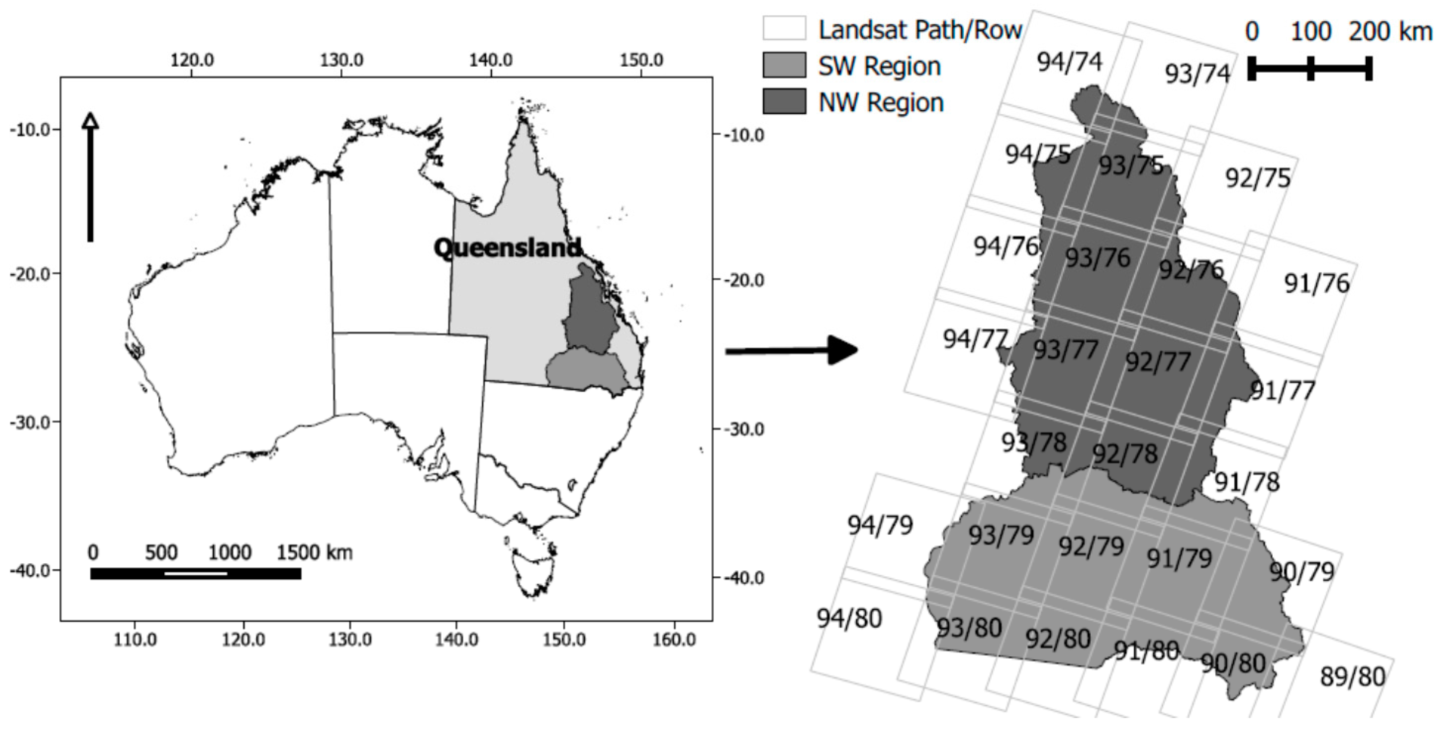
2.1. Study Area and Rationale

The study area (Figure 1) is the Western Cropping Zone (WCZ) within the State of Queensland, Australia, which is based on a strategic cropping land map by the Queensland Department of Natural Resources and Mines [39]. The WCZ major industries are mining (particularly for coal and coal seam gas) and other agricultural sectors (i.e., cropping and livestock grazing). QLUMP maps 9.7% of the total area of the western cropping region as “cropping” land, with 85.4% mapped as grazing and 0.4% as mining.

The area is summer-rainfall dominated (350–500 mm) originating from prevailing south-easterly winds, with average annual precipitation between 500 and 700 mm and a high between-season variability [40]. Cropping land use is mainly determined by the presence of highly fertile clay soils (classified mainly as Vertosols, according to the authors of [41]) and well-drained, friable clay-loam soils high in iron (ferrosols), which occur in patches [40].

Queensland’s gross value of broadacre cropping commodities for 2013–2014 were 2.7 billion dollars [42]. Over half of this is produced in the WCZ (the remainder being the coastal 1.2 billon dollar sugarcane industry). The dominant summer crops are sorghum, maize and cotton or (in the case of late summer rain) mungbeans. The dominant winter crops are wheat, barley, and chickpea [43]. Due to a strong north-south climatic gradient, the WCZ can be subdivided into “NW” (for north-western) and “SW” (south-western) regions. This gradient and division is mainly driven by increased evaporation due to latitudinal radiation increase and lower winter rainfall in the NW [40].

Some large areas of the WCZ’s most productive cropping land coincide with areas of economically viable coal. This conflicting land use has implications for food security and the long-term economic potential from agriculture. In 2014, the State Government of Queensland introduced legislation to help manage the competing land uses in areas of regional interest, including the WCZ. The Regional Planning Interests Act (RPI) 2014 aims to protect high-quality agricultural areas and areas considered to be strategic cropping land [44]. To help identify these areas, current and historical spatial information is required, particularly information and data which can identify how often, and where, cropping activity has been undertaken.

2.2. Defining the Growing Seasons

The WCZ primarily has a winter and a summer growing season [40]. We therefore aim to identify actively growing crops in these key growing seasons. For the purposes of this study, we define the summer growing season as November to May (inclusive), and the winter growing season as June to October (inclusive). When attributing a year to a summer-growing crop the most recent was used, e.g., “summer 2013” represents the period November 2012 to May 2013.

2.3. Satellite Imagery

All available Landsat 5 TM, Landsat 7 ETM+ and Landsat 8 OLI data across 27 footprints with cloud cover of less than 60% were used (Figure 2). The archived images over Australia appear only with higher image frequency since late 1987 [45]. This criterion was chosen to reduce the potential for noise in the data due to imperfect cloud/cloud shadow masking and water vapour variations.

All images were cloud-masked with a regionally adapted version of Fmask [46,47,48] then NBAR-corrected [46]; this latter step converts the units of the imagery to bottom-of-atmosphere reflectance, scaled to the interval (0, 1). The high internal geometric consistency of the USGS-based Landsat imagery allows further data processing and analysis without further geometric adjustment [28].

2.4. Synthetic Image Generation and Segmentation

All archived images were used to generate a synthetic spectral image for each season (s) and year (y). The synthetic images are denoted herein $L\left(s,y\right)$. The images were generated per pixel and per spectral band (excluding the thermal band), based on a statistical model [49] (Figure 3). Seasonal mid-points, t₀, of cropping activity were defined as 14 February for the summer growing season and 15 September for the winter growing season. These mid-points represent the times when generally the most plant vigour is expected in the study area [43].

Denote the time series of reflectance for a particular Landsat pixel and band within $L{\left(s,y\right)}_{i,j}$ with i representing the number of images within a season (i = 1, …, n); and j a single pixel. When an observation coincided with t₀ nothing more needed to be done; the reflectance value entered the synthetic image directly. Otherwise, when n = 1 a nearest-neighbour interpolation was applied to establish the reflectance value for t₀; when n > 1 we calculated, in statistical parlance, the “location” and “scale” of $L\left(s,y\right)$. For 2 ≤ n ≤ 4 location and scale were taken as the conventional mean and standard deviation, respectively; for n > 4 we invoked robust statistics, where location and scale became the median and median absolute deviation of the reflectance z at t₀. The median absolute deviation is given by the authors of [50] and gives a robust estimation of one standard deviation:

$$\text{scale}\left(L\left(s,y\right)\right)=1.4826\left\{\text{median}\left(\left|L{\left(s,y\right)}_{i,j}-\text{median}\left(L\left(s,y\right)\right)\right|\right)\right\}$$

(1)

Any observation outside the interval:

$$\text{location}\left(L\left(s,y\right)\right)\pm 2\left\{\text{scale}\left(L\left(s,y\right)\right)\right\}$$

(2)

was considered an outlier and adjusted to the interval (Figure 3). This procedure is known as Winsorising [49]. A linear regression was then fitted to the nearest four observations to t₀, with z as the response variable (reflectance), and time as the single explanatory variable. Note that Winsorising does not remove the effect of an outlier, it merely reduces its influence on subsequent analyses.

The most recent QLUMP mapping was used to mask areas from each synthetic image that were associated with land uses that were not of interest for this study (e.g., conservation areas, forestry, and intensive uses). Travelling stock routes, which are areas reserved along roadways for the movement of livestock, were also masked from each image. Water bodies were masked for each synthetic image by calculating the water index of the work in Reference [51] for each image in $L\left(s,y\right)$. If the minimum of the water index was > t_r (the recommended threshold was t_r = 68 units) it was assumed that the pixel was not covered by water during the growing season and hence left unmasked; otherwise, a one-sided Wilcoxon signed-rank test was used to determine if the median water index over the growing season was < t_r. If the null hypothesis was rejected at p < 0.05 the pixel was considered inundated for a substantial part of the growing season and masked from all further analyses.

To reflect the fact that land is managed in discrete parcels, and to reduce data loads, the (masked) synthetic images were segmented into homogeneous areas using the open-source software package RSGISLib with Python bindings [52,53]. Each synthetic image was segmented independently to account for change between seasons. The segmentation combines a k-means clustering algorithm with a clumping step to find the connected regions of the image [53]. The number of cluster centres and the minimum segment size are required input parameters. A minimum segment size of 50 pixels (4.5 ha) with 60 k-means nodes per Landsat image were used (recommended settings; [52]). Sixty nodes appeared to work best on a full Landsat image, while the minimum segment size of 50 pixels was empirically determined as a good compromise between avoiding an under splitting and too much over splitting. The segmented image was stored in the GDAL-supported KEA image format [54] where the image segments are linked with a raster attribute table (RAT) and used as the basis of all further analysis. This step is a method of data reduction by moving away from a pixel-based analysis to spatial medians per segment for all classification variables. A final step used a 1-s digital elevation model [55] to mask out segments with a slope of greater than 10% as cropping is generally not undertaken in steep terrain within the study region.

2.5. Classification Variables

A range of variables were calculated in order to capture reflectance signatures and temporal characteristics, which were used to classify the image segments (

Table 1. Remote sensing variables, computed on a per-pixel basis, that were spatially aggregated and added to the raster attribute table of the segmented synthetic images.

	Vegetation Indices, Temporal Variables and Band Ratios
1	Normalised Difference Vegetation Index (NDVI) [29]
2	Modified Chlorophyll Absorption in Reflectance Index (MCARI) [56]
3	Renormalized Difference Vegetation Index (RDVI) [57]
4	Triangular Vegetation Index (TVI) [57]
5	Modified Simple Ratio (MSR) [57]
6	Normalised Difference Burn Ratio (NDBR) [58]
7	NDVI seasonal variance (ndviTsVr)
8	NDVI seasonal minimum (ndviTsMn)
9	NDVI seasonal maximum (ndviTsMx)
10	NDVI seasonal coefficient of variation (ndviTsCV)
11	NDVI seasonal range (ndviTsRng)
12	NDVI gradient up (first minimum to maximum) (ndviTsGr1)
13	NDVI gradient down (maximum to second minimum) (ndviTsGr2)
14	NDVI day of time series maximum (ndviTsDyMx)
15	b7 − b3/(b7 + b3) (nr73)
16	b7 − b2/(b7 + b2) (nr72)
17	b5 − b7/(b5 + b7) (nr57)
18	b4 − b5/(b4 + b5) (nr45)
19	b5 − b3/(b5 + b3) (nr53)
20	b5 − b2/(b5 + b2) (nr52)
21	b4 − b2/(b4 + b2) (nr42)
22	b2/b3 (r23)
23	b4/b3 (r43)

). Firstly, the mid-season values for a number of vegetation indices and band ratios were calculated for the pixel-based mid-season synthetic image. Similarly, pixel-based NDVI values were calculated from the mid-season synthetic image, as well as descriptions of several temporal metrics (Table 1). The RATs were populated with the spatial median per segment for each variable listed in Table 1.

A final variable was created based on the land use data from QLUMP [24] to help constrain the classification to known areas of cropping. All areas classified as “cropping” were extracted from the QLUMP mapping data to create a mask of cropping areas. It is important to note that, due to the limited temporal information that is used for mapping cropping areas in the QLUMP, these areas classified as cropping may not be a comprehensive spatial representation of all areas of active cropping over time. Hence, while being a potentially useful explanatory variable for classification purposes, the land use mapping was not used as an explicit representation of all cropping in the study area. The metrics used here are specifically targeted to distinguish the Crop/No-Crop classes and differ from, e.g., the authors of [8,30] who aimed for a more general land use classification.

2.6. Training and Validation Data

Field-based training data described in Reference [43] was used in this study. These data, collected from various campaigns between September 1999 and February 2012, include observations about presence and absence of crop (e.g., wheat, maize, sorghum, etc.) at the time of observation. For the purpose of this study, all records were recoded as either Crop or No-Crop. The field data were intersected spatially and temporally with the image segments from each synthetic mid-season image. When more than one observation fell within the same image segment only the first was retained and only if the observations belonged to the same class (Crop or No-Crop); if they had different classes none of the observations were used.

An additional set of records were generated through desktop interpretation of the seasonal synthetic images. The sites were sampled at random over space, growing seasons, and years. The intention of these records was to provide an unbiased assessment of cropping activity that could serve as validation data. From a desktop, an expert would “visit” a sampled location in space-time and use $L\left(s,y\right)$ data (and any other higher-resolution imagery if available) to assess whether the on-ground activity was either Crop or No-Crop. Occasionally the sampled spatial coordinate fell on a field boundary or road; in this case, the coordinate was manually moved inside the nearest field (but never more than a distance greater than 3 pixels).

These records form a set of explanatory variables and a response variable amenable to statistical modelling. A breakdown of the numbers of training and validation data is shown in

Table 2. The number of training and validation data used, separated by growing season and region.

Summer	Crop	No-Crop	Crop	No-Crop	Crop	No-Crop
	Training	Training	Validation	Validation	Total	Total
NW	280	1215	58	1359	338	2574
SW	547	732	113	1245	660	1977
Winter	Crop	No-Crop	Crop	No-Crop	Crop	No-Crop
	training	training	validation	validation	total	total
NW	145	1309	68	1292	213	2601
SW	448	758	181	1236	629	1994

. In NW 51% and 52% for summer and winter, respectively, were derived from the collated field data. For SW the field data accounted for 49% and 46% of the total data set for summer and winter, respectively.

The number of validation data points for the class Crop is relatively small (Table 2). The random sampling approach (with 9.7% of the study area being mapped as “cropping” by the QLUMP) does imply that about 10% of the validation data should be Crop if all areas are actively cropped at all times. The class Crop is, however, in the validation dataset represented with an even smaller percentage, resulting in an unbalanced dataset. Table 2 reflects this distribution and implies that a validation based on these data is, due to the small number of points for the class Crop, potentially misleading. Due to the intensive field sampling and farm surveys, more data on the actively cropped fields is available in the training data. Therefore, for the purpose of training and validation, the original validation data were merged with the original training data. A 75% random subsample of the merged data was chosen for the model training and the remaining 25% subsample quarantined for validation. Thus, a total 1387 points were used for validation in summer and 1359 in winter across the regions.

2.7. Image Classification

The generation of a categorical classification generally has the underlying assumption that the features in question can be systematically separated into distinct classes by their numerical properties. The classes in a supervised classification are specified a priori, and associated with a set of training data for each class. A wide range of algorithms exists to choose from, each with their specific advantages and disadvantages. The authors of [59] tested 179 different classification models arising from 17 classification families on 121 different datasets, to answer the question if we always need to apply multiple classifiers and choose the best performing algorithm. They came to the conclusion that Random Forest (RF) [60] is most likely performing best, but with no significant improvement over the second-best performing algorithm, Support Vector Machines (SVM) [61]. In this approach we compared four classification algorithms with the same training data: (i) SVM; (ii) multinominal logistic regression; (iii) the decision-tree classifier C5.0 ([62]; and (iv) RF; all within the R software. Table 1 describes the explanatory variables spanning the classification feature space. A total of 23 variables were generated for each region and season.

• In a (non-linear) SVM classification the feature space is transformed to a higher dimension using what is called a “kernel trick”, where a hyperplane is fitted to separate the different classes [61,63], which may not be feasible in the lower dimensional space.
• Multinominal logistic regression (also called the multinomial logit model) can be used when the dependent variable is categorical, and thus for classification problems [64]. The multinomial logit model (referred to as “Logit” from here on) assumes that dependent variables cannot be perfectly predicted from the independent variables, but that a linear combination of training data can be used to determine the probability of each outcome.
• The C5.0 decision-tree classifier was originally a commercial tree-based classifier that was introduced by the authors of [65], made publicly available in 2011 and described in detail by the authors of [62].
• RF is a method suitable for classification applications that constructs a multitude of decision trees [60,66]. RF is a way of averaging multiple single trees trained on slightly different sub-samples of the training data. This “bootstrapping” step generally leads to a better model performance by reducing the variance without introducing bias. This also means that, while a single tree may be subject to noise in the input data, the average is not (as long as the trees are not correlated). These features of the RF were further explored in an offline analysis: a single RF tree was selected as a classifier, as well as a single RF pruned tree, and a RF trees with Bayesian bagging (single and pruned). The single trees and Bayesian bagging did not result in improved classification accuracy and was not further investigated due to the processing cost. Within the RF classifier was land use “cropping” extracted from QLUMP and used as an a priori variable (as a factor) in the suite of classification approaches (RF + land use).

For each of the classifiers used, the probabilities of the class membership were stored per image segment. Each segment was labelled as Crop if the predicted probability for that segment was greater than 0.5, due to the binary nature of the classification.

The classification is performed ensemble for all years per season and region, to account for inter-annual variability in the cropping and for years without field data.

3. Results

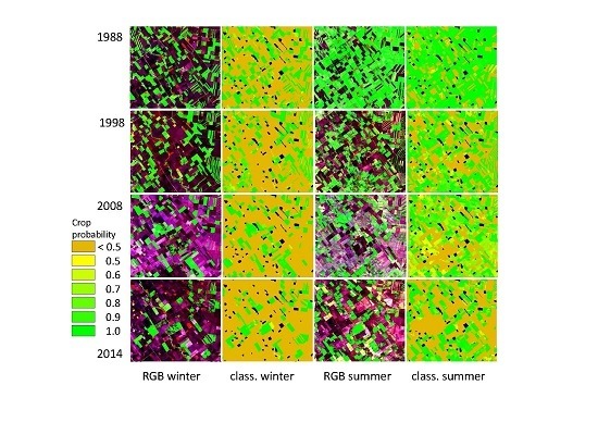
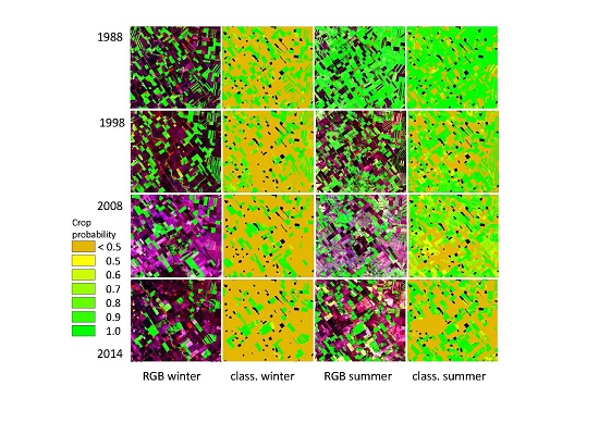
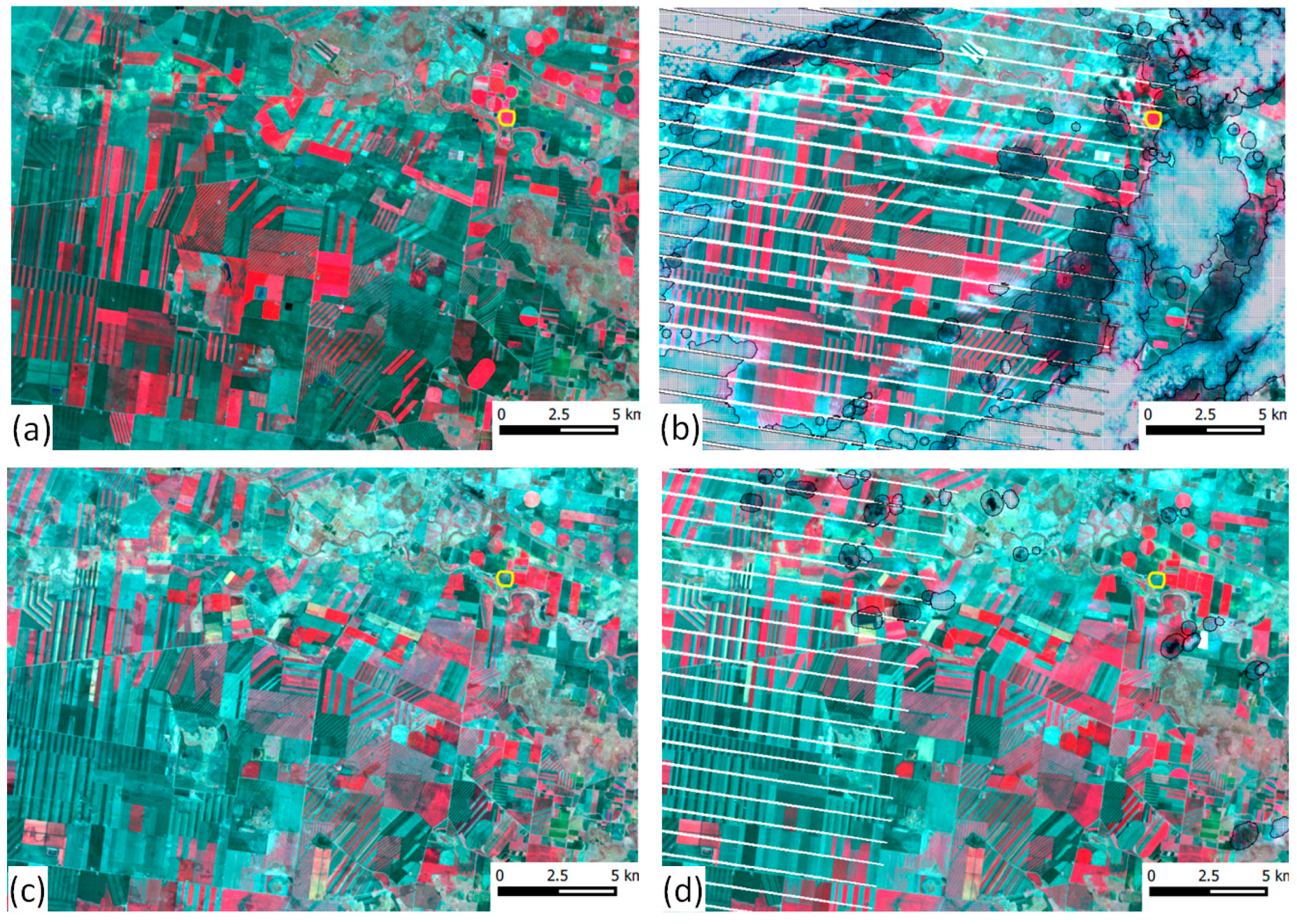
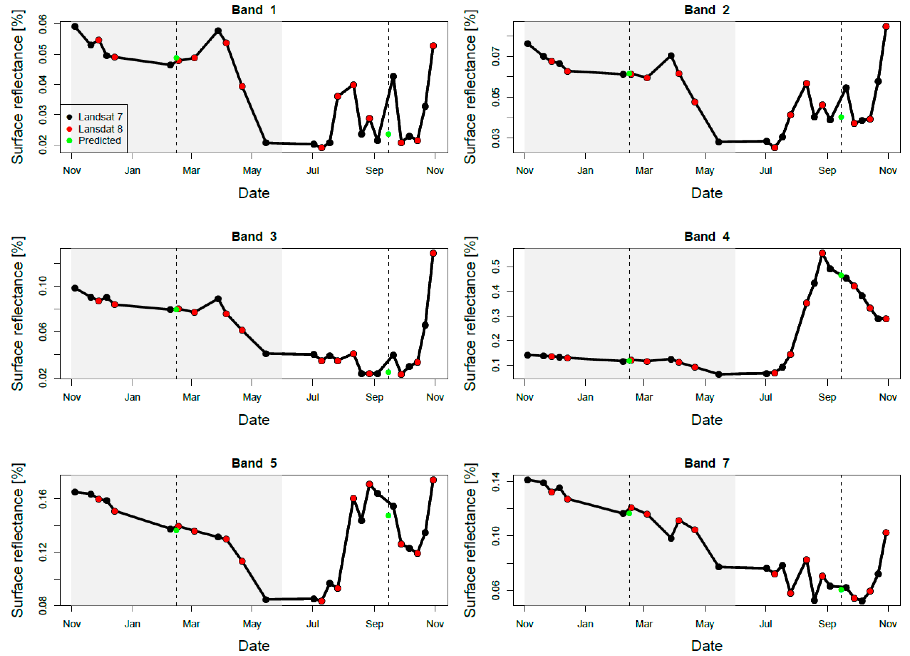
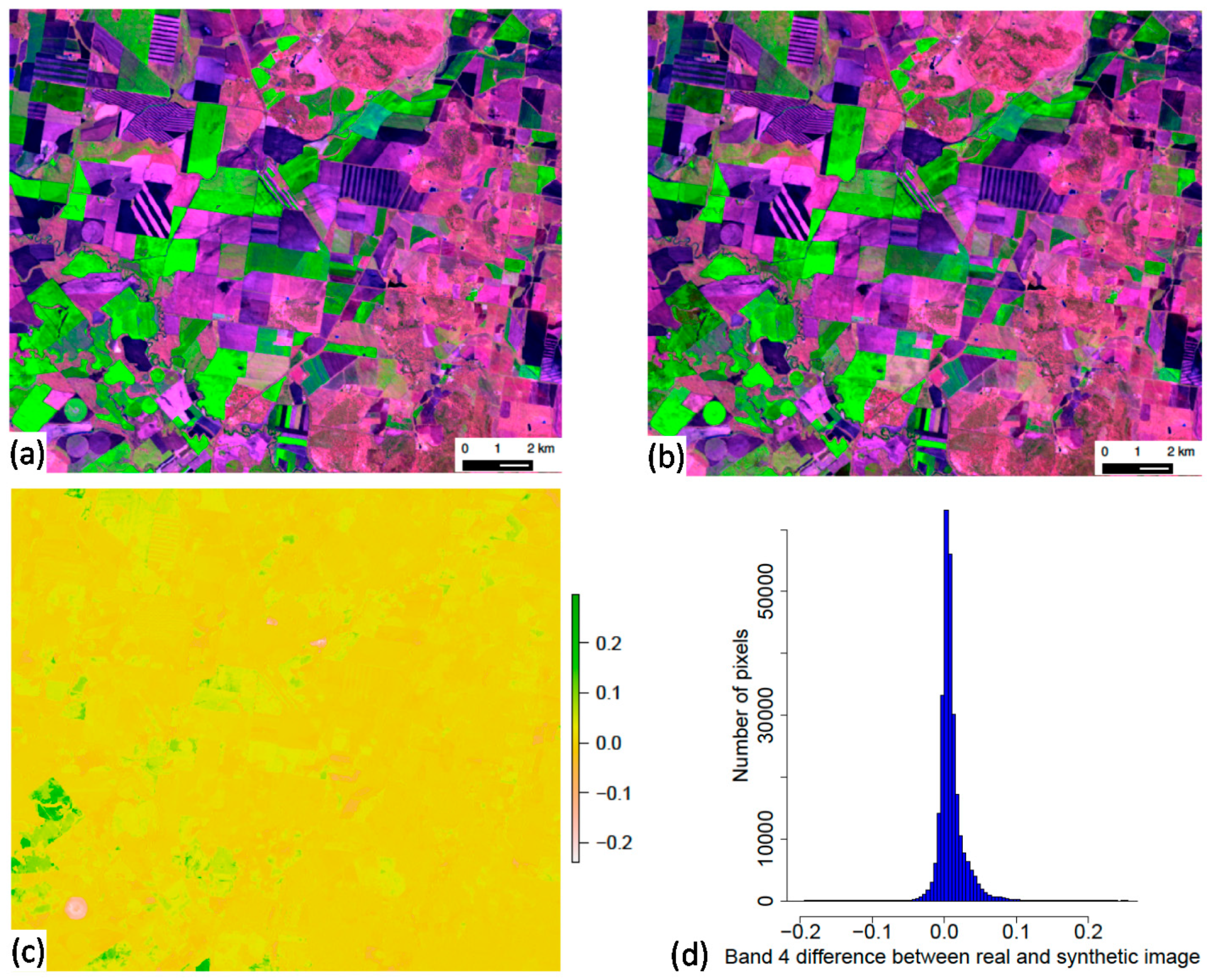
3.1. Synthetic Image Generation

Figure 4a,c provide examples of the mid-season synthetic images for a subset of the SW region for the winter growing season and the summer growing season, respectively. Figure 4b,d show the respective single-date images closest to the mid-season date (in this case both Landsat 7). Both images contain clouds with different degrees of image contamination with the Fmask based cloud and cloud shadow polygons overlaid. The robust seasonal synthetic image algorithm appears to work well; even if at times artefacts can be found, e.g., if scan-line correction (SLC) is off in Landsat 7 ETM+ or if the temporal gap between images is large (i.e., due to changes in vegetative phenology).

The temporal behaviour of a crop in relation to the synthetic image is graphically illustrated in Figure 5 for a centre pivot circle (yellow outline in Figure 4a), which is fallow in summer 2014 and irrigated in the following winter 2014. The green data point marks the predicted value at the mid-season date, while the red data points represent Landsat 8 OLI and the black data points Landsat 7 ETM+ spatially averaged (over the extent of the circle) data values.

Figure 5 demonstrates that the prediction point for summer is well aligned with the Landsat observations, while prediction point for winter 2014 has some deviation, particularly in Bands 1 to 3, due to the effects of clouds and SLC-off. Generally though, the predicted green points are in line with the temporal behaviour of the curve. This suggests that Bands 1 to 3 are likely to have been affected by other factors including variations in atmospheric constituents, such as water vapour in decreasing magnitude [46,47]. The synthetic image generation based on the Winsorising approach appears to have filtered the effects of contamination, and retained the overall trend.

The quality of the synthetic image generation was evaluated in an image subset for scene 90/79. The synthetic image was generated without the image observation on 15 September 2015 (Figure 6a). The synthetic image (Figure 6b) resembles the real image fairly well as the difference map (Figure 6c) indicates. The major differences visible are a crop circle, where the band 4 reflectance was overestimated (lower left) and some close by fields which were underestimated. Both of these cases are due to the phenological changes in the latest image selected in the prediction (9 October). The majority of the differences in band 4 is between ± 0.05, which is similar to the synthetic image generation by the authors of [35]. A regression between the observation and synthetic image revealed a residual standard error of 0.021 with an adjusted r² of 0.95 (p < 0.00001).

Despite the (minor) differences in greenness was the synthetic image considered adequate for GEOBIA.

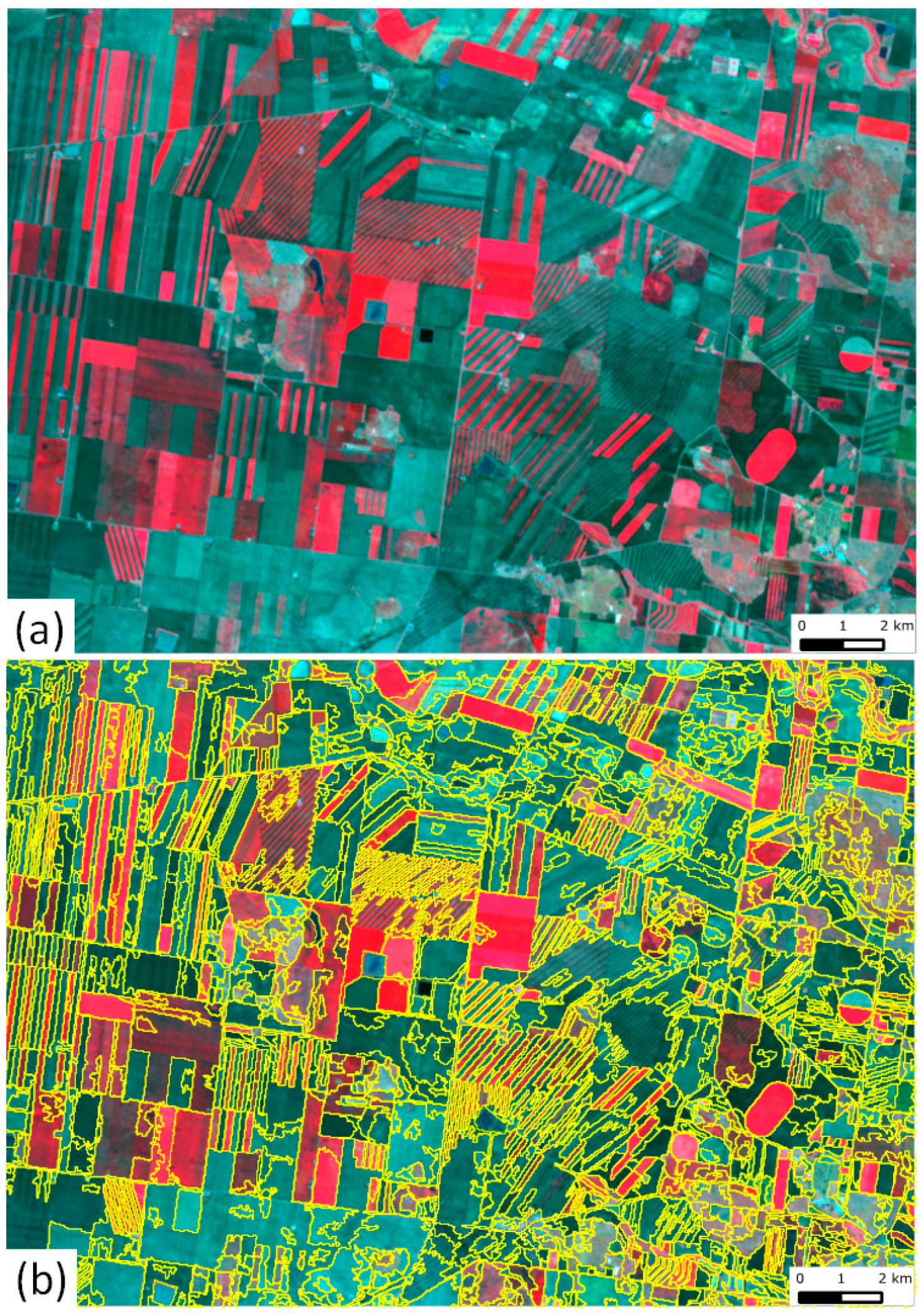
3.2. Image Segmentation

The spatial consistency of the cloud-free synthetic image enables the application of an image segmentation approach. Each synthetic image over time is segmented independently, as field sizes and shapes may vary. Figure 7 illustrates the result of GEOBIA over a complex and heterogeneous area within the same image subset as used in Figure 3. The amount of strip cropping seen here is an extreme example of image heterogeneity within the study region.

The majority of the landscape features and field outlines are captured by GEOBIA. Some larger fields are represented boundary sharp as individual segments. The segmentation parameters appear to not separate the strips at the highest level of detail, e.g., if the strip cropping is very narrow (i.e., 1–3 pixels wide). Within-field variation can cause the algorithm to split one field or pivot circle if the heterogeneity is high [33]. This over splitting issue does not pose a problem for the overall approach as the spatially aggregated values are classified as Crop or No-Crop only. The median number of segments per Landsat path/row in NW was 74,514 and 79,861 in SW, with a median area of 873 ha and 879 ha, respectively.

The image segments for the cropped field may not always be sharp on the field boundaries so that some discrepancies with the true field outlines are apparent. This may especially when viewing the classifications over time result in some fuzziness at these borders.

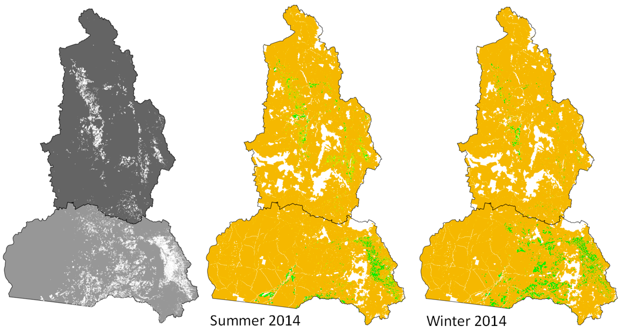
3.3. Classification and Map Accuracies

Figure 8 represents an example of the image classification for several seasons, based on the (RF + landuse) classification. The full time series of the subset is shown in the Appendix as Figure A1. The same image stretch has been applied to the mid-season synthetic images, while the probabilities for active crop are colour-coded according to the legend in Figure 8 (yellow to green). The comparison of the mid-season synthetic image is effective if the crops are greening-up during this particular time, but if a crop is planted late, e.g., due to a late summer rain, the crop might not appear green in the synthetic image. This appears to be the case for the majority of fields, but for an accurate assessment all of the seasonal imagery have to be assessed as the general peak vegetation date does not necessarily coincide with the real maximum of vegetation greenness.

Table 3. User’s and Producer’s accuracies are given for the Crop/No-Crop classification as well as the overall accuracy and the Kappa coefficient. The validation is performed separately for each region (NW and SW) and season (summer and winter). The validation was performed including all years with the 95% confidence intervals in brackets.

NW Summer
Class	Accuracy	C5.0		SVM		Logit		Random Forest (RF)		RF + landuse
Crop	Producer‘s acc.	0.580	(0.469, 0.682)	0.959	(0.848, 0.992)	0.734	(0.606, 0.833)	0.869	(0.752, 0.937)	0.878	(0.782, 0.936)
Crop	User‘s acc.	0.638	(0.521, 0.739)	0.588	(0.471, 0.694)	0.588	(0.471, 0.694)	0.663	(0.547, 0.762)	0.900	(0.807, 0.952)
No-Crop	Producer‘s acc.	0.954	(0.933, 0.968)	0.951	(0.930, 0.965)	0.950	(0.929, 0.964)	0.959	(0.939, 0.972)	0.987	(0.974, 0.994)
No-Crop	User‘s acc.	0.942	(0.920, 0.958)	0.997	(0.987, 0.999)	0.973	(0.956, 0.983)	0.987	(0.974, 0.994)	0.984	(0.970, 0.992)
	Overall Acc.	0.908	(0.883, 0.927)	0.951	(0.932, 0.965)	0.930	(0.908, 0.947)	0.951	(0.932, 0.965)	0.975	(0.959, 0.984)
	Kappa	0.555		0.704		0.615		0.725		0.875
NW Winter
Class	Accuracy	C5.0		SVM		Logit		Random Forest (RF)		RF + landuse
Crop	Producer‘s acc.	0.875	(0.740, 0.948)	0.939	(0.821, 0.984)	0.893	(0.774, 0.955)	0.922	(0.802, 0.974)	0.893	(0.774, 0.955)
Crop	User‘s acc.	0.792	(0.655, 0.887)	0.868	(0.740, 0.940)	0.943	(0.833, 0.985)	0.887	(0.762, 0.953)	0.943	(0.833, 0.985)
No-Crop	Producer‘s acc.	0.983	(0.968, 0.991)	0.989	(0.976, 0.995)	0.995	(0.985, 0.998)	0.991	(0.978, 0.996)	0.995	(0.985, 0.998)
No-Crop	User‘s acc.	0.991	(0.978, 0.996)	0.995	(0.985, 0.998)	0.991	(0.978, 0.996)	0.994	(0.982, 0.997)	0.991	(0.978, 0.996)
	Overall Acc.	0.975	(0.960, 0.985)	0.986	(0.972, 0.992)	0.987	(0.974, 0.993)	0.986	(0.972, 0.992)	0.987	(0.974, 0.993)
	Kappa	0.818		0.894		0.910		0.896		0.910
SW Summer
Class	Accuracy	C5.0		SVM		Logit		Random Forest (RF)		RF + landuse
Crop	Producer‘s acc.	0.841	(0.777, 0.900)	0.892	(0.834, 0.933)	0.922	(0.868, 0.956)	0.860	(0.781, 0.893)	0.958	(0.911, 0.981)
Crop	User‘s acc.	0.851	(0.788, 0.898)	0.856	(0.793, 0.903)	0.885	(0.826, 0.927)	0.879	(0.813, 0.917)	0.908	(0.853, 0.945)
No-Crop	Producer‘s acc.	0.941	(0.913, 0.960)	0.944	(0.917, 0.963)	0.955	(0.931, 0.972)	0.952	(0.923, 0.967)	0.964	(0.942, 0.978)
No-Crop	User‘s acc.	0.936	(0.908, 0.957)	0.959	(0.935, 0.975)	0.970	(0.950, 0.983)	0.943	(0.909, 0.957)	0.984	(0.966, 0.993)
	Overall Acc.	0.912	(0.886, 0.933)	0.930	(0.906, 0.948)	0.946	(0.941, 0.961)	0.925	(0.893, 0.939)	0.963	(0.944, 0.976)
	Kappa	0.784		0.825		0.866		0.817		0.906
SW Winter
Class	Accuracy	C5.0		SVM		Logit		Random Forest (RF)		RF + landuse
Crop	Producer‘s acc.	0.912	(0.853, 0.949)	0.954	(0.904, 0.979)	0.954	(0.904, 0.979)	0.967	(0.919, 0.987)	0.980	(0.938, 0.994)
Crop	User‘s acc.	0.973	(0.928, 0.991)	0.980	(0.937, 0.994)	0.980	(0.937, 0.994)	0.973	(0.928, 0.991)	0.980	(0.938, 0.994)
No-Crop	Producer‘s acc.	0.991	(0.975, 0.997)	0.993	(0.978, 0.998)	0.993	(0.978, 0.998)	0.991	(0.975, 0.997)	0.993	(0.979, 0.998)
No-Crop	User‘s acc.	0.969	(0.947, 0.982)	0.985	(0.967, 0.993)	0.985	(0.967, 0.993)	0.989	(0.972, 0.995)	0.993	(0.979, 0.998)
	Overall Acc.	0.970	(0.952, 0.981)	0.983	(0.968, 0.991)	0.983	(0.968, 0.991)	0.985	(0.970, 0.992	0.990	(0.977, 0.995)
	Kappa	0.922		0.956		0.956		0.960		0.973

shows the accuracy statistics for each of the five classification approaches and for each region and growing season. The same training and validation data were used for each classifier. It is important to note that the classifiers were trained and validated over all years for which data were available.

In some instances gave SVM and Logit the superior classification results, but overall the RF classifiers were always amongst the better performing. The inclusion of the prior information derived from land use mapping improved the classification accuracy considerably for summer, especially the user’s accuracy of the class Crop. To visualise the variable importance the MeanDecreaseGini metric [60,64] is displayed (Figure 9). This is a measure of variable importance based on the Gini impurity index used for the calculation of splits during RF training. Every time a node split is made in the RF based on an explanatory variable, the Gini impurity criterion for the two descendent nodes is less than the parent node. Adding up the Gini decreases for each explanatory variable over all trees in the forest gives an importance measure that is often very consistent with the permutation importance measure [60,64]. Figure 9 plots the 10 most important variables in the four cases (NW and SW in summer and winter).

In the NW subzone, for summer and winter, there are 6 temporal metrics within the 10 most important variables; in the SW subzone 5 out of the 10 most important were temporal metrics. It is also revealed that, in summer, prior knowledge of land use is an important aspect of the classification.

The (RF + landuse) classification was applied to all seasons and years. Figure 10 shows an example of the crop probabilities predicted for the WCZ for the summer and winter growing season of 2014.

The classified surfaces are available for all season and years (1988–2015) for download via the Terrestrial Ecosystem Research Network website ([67,68]).

Summarising the active crop history over a defined period of time can give an insight of the spatial distribution of the crop activities and intensities of use over last 27 years. This is visualised in an image subset in Figure 11, where the intensive use in the summer irrigation near a river stands out in the long-term cropping count (Figure 11f).

Figure 11 also indicates the different land use interests with the open-cut coal mine Acland mining lease of stage 1 in 2005 outlined in blue and subsequent extension leases including a rail line. The stage 3 extension was approved (with conditions) in 2012 and is currently under review by the Queensland Department of State Development Infrastructure and Planning [69] which entails an environmental impact assessment. The use of the historic imagery and in particular the active crop frequency layers will be investigated for updating the existing land use data.

A field that was not part of the most recent land use layer as outlined in Figure 12 was captured as cropped multiple times in the 20-year period of 1995–2014.

The image segments for the cropped field may not always be sharp on the field boundaries so that some discrepancies with the true field outlines are apparent. This may especially be the case when viewing the classifications over time, resulting in some fuzziness at the borders.

4. Discussion

4.1. Synthetic Image Generation and Segmentation

The synthetic image generation step is vital for the subsequent analysis as the image segments and some of the indices used in the classification are based on this. For the majority of seasons there are 10 or more Landsat images with less than 60% cloud cover. The threshold was applied to reduce the risk of image artefacts from imperfect cloud and cloud-shadow masking, thin undetected clouds and water vapour variations which can influence an individual pixel’s reflectance values. Only a few footprints in a specific growing season have fewer than five images available. Too few images per season may lead to artefacts in the synthetic image generation and unrealistic temporal metrics and thus reduce the overall accuracy. This could only be overcome in some regions by carefully selecting and including additional scenes with higher cloud cover, or if further Landsat imagery would be available from yet unknown Landsat archives.

The GEOBIA used here is well-suited to both the broadacre cropping areas and the smaller, more heterogeneous fields (Figure 7). Over-splitting of the segments can occur due to within-field spatial heterogeneity, or in cases where the base image displays stripes originating from ETM+ SLC-off data. The over-splitting, however does not pose a problem to the classification as these polygons are attributed and classified separately. Under-splitting may occur, if the field sizes due to strip-cropping become small (e.g., a few pixels in width) or, e.g., if field boundaries are diffuse [33]. A more detailed segmentation could help to separate these strips further. This could include a regionally adapted parameter setting (e.g., for the minimum segment size), but would most likely require higher spatial resolution imagery. This may become important for a crop type classification, but in our case for a binary Crop/No-Crop classification this is not as relevant, so one setting with a large number of clusters per Landsat footprint was used in the segmentation. The authors of [32] performed an “individual crop field” accuracy assessment with reference polygons while using a five-year composited image product to gain more defined image boundaries on repeatedly cropped fields. Accurate field delineation is not a primary focus of this study, but outputs of this classification are envisaged to feed into the QLUMP system to aid the updating of land use and potentially field boundaries.

The approach applied here is designed for large-area mapping and our results indicate that mapping at field-scale works with acceptable accuracy. In the spatial aggregation step, spatial median values have been calculated, making the approach more robust against spatial outliers such as pixels affected by imperfect cloud or cloud-shadow masking. One of the benefits of the GEOBIA is that there is no removal of “salt and pepper” effects required [33,37].

4.2. Classification Performance and Map Accuracies

NDVI was used as the primary vegetation index for the temporal metrics. The Enhanced Vegetation Index (EVI) is commonly used for vegetation studies [70] to reduce the effect of soil. As we are not comparing absolute values of a vegetation index across large spatial extents, rather the temporal signal in a relative manner over time, NDVI is just as useful, as the soil is not changing drastically over time for each location (three decades). A similar argument applies for a potential cross-calibration of the Landsat 5/7 with Landsat 8 NDVI, which was discarded in this case: the authors of [46] investigated the difference in NDVI and found an up-to-5% discrepancy between Landsat 7 and 8. When applying a correction factor the difference was reduced to 1% across all Australian natural landscapes. This suggests that for NDVI estimates, the difference between the two instruments is small. The difference may yet be smaller in the cropping systems with different biophysical properties so that an improvement is not guaranteed at this stage, but should be investigated in the future.

A vegetation cover description with an entire different approach, such as spectral mixture analysis [71] may add additional information and will be investigated further. The temporal metrics are, however, among the most important variables in the classification.

The comparison of classification algorithms revealed that the SVM classifier and the RF classifier perform similarly. This is supported in the findings of Reference [59] and, following their recommendation and the results obtained from the classification, the RF classifier was used. While a particular classifier may perform slightly better (i.e., SVM) for a season or year, one classifier was chosen for all cases for the purpose of processing speed, comparability and consistency, given the large areas and longer time series over which the approach was to be applied.

We found that, in the absence of land use information, it was difficult to predict Crop with adequate accuracy in summer. This is because annual pastures tend to grow with summer rainfall events, resulting in increased greenness, and hence classification confusion. Similarly, in years with unusually high rainfall (e.g., the winter growing season of 2007), an overestimation of cropping activity occurs as pastures can show a rapid vegetative response. Actively growing crops can therefore be confused with pastures or improved pastures, particularly where the pasture growth is further promoted by irrigation (e.g., for hay production). This is reflected in the improvement in the (RF + landuse) model in the users accuracy for the class Crop in summer for both regions (about 14% in NW and 3% in SW). The class probabilities for the class Crop were mapped and colour-coded. A probability threshold of 0.5 was applied globally as a demarcation in the binary classification. In some areas a local adjustment of the probabilities might result in a better crop differentiation. The inclusion of land use as an explanatory variable comes at no real cost to the model and, with the exception of the NW winter (where the producers accuracy is reduced by 2%), the overall accuracies are improved, especially in the summer season (Table 3) i.e. user’s acc. in NW summer. In the case of a large time difference between the land use mapping and the crop-mapping date, a false weighting may result in mis-classification. Incorporating historic land use maps, where they exist, may reduce this effect, although historic maps may differ in scale and accuracy compared with more recent mapping. It could be argued that an accuracy improvement of about 1% in NW winter or in SW winter does not warrant the (RF + landuse) model over RF, however for consistency, the same model was used for each region and season. While the land use mapping was included here as a variable, the classification results suggest that in the absence of a land use map, the RF approach would still achieve reasonable results.

The classification accuracies based on the Kappa statistic are between 0.88 and 0.97 suggesting that a good separation between the grazing land and active cropping can be achieved. More validation data are desirable, especially for the class Crop, where the data set is unbalanced due to the small proportion of the cropping in the study area (9.7% according to the land use map). The statistics reveal that in the NW sub-zone the producer’s accuracy for the class Crop in the summer growing season is the lowest at 0.88, while for NW and SW summer the user’s accuracies for Crop are the lowest with 0.90 and 0.91 (Table 3).

4.3. Future Applications

Based on our mapping of cropping activity, further developments are planned. This includes testing a crop-type classification, and then extending that to yield mapping and forecasting through the incorporation of climate information and other sources of Earth-observation data, such as Sentinel-1 and 2. Gaps in the image archive can pose a problem for the procedure, particularly when the 16-day gap between Landsat observations coincides with a period of dense cloud cover. Regularly spaced observations would allow for a phenology-based approach that also has the potential for crop-type differentiation [43], but might require an image-fusion step to be applicable at field-scale—for example Landsat with MODIS data [72]; [73] or Rapideye and MODIS [74]. The authors of [75] demonstrated the use of multispectral Landsat information combined with temporal MODIS information for crop mapping. The authors of [76] used a MODIS- and Landsat-fused time series to investigate tillage management practices in agricultural systems. A potential drawback can be the loss in spectral “sharpness” [76,77] in the fused data and the large data volume. The maps produced are available online an can be used as independent data to validate coarse-resolution crop mapping approaches at a continental or global scale [16].

The advent of the European Space Agency’s Sentinel-2 imagery is expected to increase the classification accuracy, as more observations per season are expected combined with a finer spatial resolution. The classification procedure is based on simple vegetation indices and band ratios so that data from different sensors can easily be integrated and new seasonal crop maps can be generated. Further, the integration of Landsat Multi Spectral Scanner data would extend the crop mapping approach back to 1972, but larger temporal gaps in the data may require a different approach [78].

The data generated and the framework as such could be considered for crop mapping approaches within GEOGLAM (Group on Earth Observations Global Agricultural Monitoring Initiative).

5. Conclusions

The full Landsat data archive from 1987–2015 of TM/ETM+/OLI imagery were used to create maps of cropping activity for the summer and winter growing seasons for each year (starting in the southern winter of 1988) in the Western Cropping zone of Queensland, Australia. The approach is based on a flexible, per-season image segmentation, followed by a classification that uses temporal metrics, spectral indices and land use mapping as explanatory variables. Several machine-learning techniques were compared, and random forest was generally superior. The most important variables in the classification were NDVI range, NDVI coefficient of variation and land use. The Classification accuracies (Kappa statistic) for this binary Crop/No-Crop classification were 0.88 and 0.91 in northern part of our study area during the summer and winter growing seasons, respectively. In the southern part of the study area, the Kappa statistic was 0.91 and 0.97 for summer and winter, respectively. The results suggest that, with appropriate training and validation data, the approach developed and applied here is suitable for large-area mapping of cropping activity using the Landsat archive. It is also expected that the approach would be transferable to other satellite imagery with sufficient spatial, spectral and temporal resolution to generate the explanatory variables used in this study.

The resulting classified imagery and crop frequency maps for the period of 1988 to 2015 for both summer and winter season are available online via: References [67,68].

References

1. Grassini, P.; van Bussel, L.G.J.; Wart, J.V.; Wolf, J.; Claessens, L.; Yang, H.; Boogaard, H.; de Groot, H.; van Ittersum, M.K.; Cassman, K.G. How good is good enough? Data requirements for reliable crop yield simulations and yield-gap analysis. Field Crops Res. 2015, 177, 49–63. [Google Scholar] [CrossRef] [Green Version]
2. Rembold, F.; Atzberger, C.; Savin, I.; Rojas, O. Using Low Resolution Satellite Imagery for Yield Prediction and Yield Anomaly Detection. Remote Sens. 2013, 5, 1704–1733. [Google Scholar] [CrossRef] [Green Version]
3. Chipanshi, A.; Zhang, Y.; Kouadio, L.; Newlands, N.; Davidson, A.; Hill, H.; Warren, R.; Qian, B.; Daneshfar, B.; Bedard, F.; et al. Evaluation of the Integrated Canadian Crop Yield Forecaster (ICCYF) model for in-season prediction of crop yield across the Canadian agricultural landscape. Agric. For. Meteorol. 2015, 206, 137–150. [Google Scholar] [CrossRef]
4. Atzberger, C. Advances in Remote Sensing of Agriculture: Context Description, Existing Operational Monitoring Systems and Major Information Needs. Remote Sens. 2013, 5, 949–981. [Google Scholar] [CrossRef]
5. Foley, J.A.; DeFries, R.S.; Asner, G.P.; Barford, C.; Bonan, G.; Carpenter, S.R.; Chapin, F.S.; Coe, M.T.; Daily, G.C.; Gibbs, H.K.; et al. Global Consequences of Land Use. Science 2005, 309, 570–574. [Google Scholar] [CrossRef] [PubMed]
6. Hilson, G. An overview of land use conflicts in mining communities. Land Use Policy 2002, 19, 65–73. [Google Scholar] [CrossRef]
7. Godfray, H.C.J.; Beddington, J.R.; Crute, I.R.; Haddad, L.; Lawrence, D.; Muir, J.F.; Pretty, J.; Robinson, S.; Thomas, S.M.; Toulmin, C. Food Security: The Challenge of Feeding 9 Billion People. Science 2010, 327, 812–818. [Google Scholar] [CrossRef] [PubMed]
8. Hansen, M.C.; Defries, R.S.; Townshend, J.R.G.; Sohlberg, R. Global land cover classification at 1 km spatial resolution using a classification tree approach. Int. J. Remote Sens. 2000, 21, 1331–1364. [Google Scholar] [CrossRef]
9. Herold, M.; Mayaux, P.; Woodcock, C.E.; Baccini, A.; Schmullius, C. Some challenges in global land cover mapping: An assessment of agreement and accuracy in existing 1 km datasets. Remote Sens. Environ. 2008, 112, 2538–2556. [Google Scholar] [CrossRef]
10. Cracknell, A.P. The Advanced Very High Resolution Radiometer; Taylor and Francis: London, UK, 1997. [Google Scholar]
11. Schmidt, M.; King, E.A.; McVicar, T.R. Assessing the geometric accuracy of AVHRR data processed with state vector based navigation as implemented in CAPS (Common AVHRR Processing System). Can. J. Remote Sens. 2008, 34, 496–508. [Google Scholar] [CrossRef]
12. Justice, C.O.; Townshend, J.R.G.; Kalb, V.L. Representation of Vegetation by Continental Data Sets Derived from NOAA-AVHRR Data. Int. J. Remote Sens. 1991, 12, 999–1021. [Google Scholar] [CrossRef]
13. Quarmby, N.A.; Townshend, J.R.G.; Settle, J.J.; White, K.H.; Milnes, M.; Hindle, T.L.; Silleos, N. Linear mixture modelling applied to AVHRR data for crop area estimation. Int. J. Remote Sens. 1992, 13, 415–425. [Google Scholar] [CrossRef]
14. Atkinson, P.M.; Cutler, M.E.J.; Lewis, H. Mapping sub-pixel proportional land cover with AVHRR imagery. Int. J. Remote Sens. 1997, 18, 917–935. [Google Scholar] [CrossRef]
15. Schmidt, M. Development of A Fuzzy Expert System for Detailed Land Cover Mapping in the Dra Catchment (Morocco) Using High Resolution Satellite Images. Ph.D Thesis, University of Bonn, Bonn, Germany, 2003. [Google Scholar]
16. Atzberger, C.; Rembold, F. Mapping the Spatial Distribution of Winter Crops at Sub-Pixel Level Using AVHRR NDVI Time Series and Neural Nets. Remote Sens. 2013, 5, 1335–1354. [Google Scholar] [CrossRef] [Green Version]
17. Friedl, M.A.; McIver, D.K.; Hodges, J.C.F.; Zhang, X.Y.; Muchoney, D.; Strahler, A.H.; Woodcock, C.E.; Gopal, S.; Schneider, A.; Cooper, A.; Baccini, A.; Gao, F.; Schaaf, C. Global land cover mapping from MODIS: Algorithms and early results. Remote Sens. Environ. 2002, 83, 287–302. [Google Scholar] [CrossRef]
18. Lymburner, L. The National Dynamic Land Cover Dataset; Geoscience Australia: Symonston, Australia, 2011.
19. Lobell, D.B.; Asner, G.P. Cropland distributions from temporal unmixing of MODIS data. Remote Sens. Environ. 2004, 93, 412–422. [Google Scholar] [CrossRef]
20. Maxwell, S.K.; Sylvester, K.M. Identification of “ever-cropped” land (1984–2010) using Landsat annual maximum NDVI image composites: Southwestern Kansas case study. Remote Sens. Environ. 2012, 121, 186–195. [Google Scholar] [CrossRef] [PubMed]
21. Homer, C.G.; Dewitz, J.A.; Yang, L.; Jin, S.; Danielson, P.; Xian, G.; Coulston, J.; Herold, N.D.; Wickham, J.D.; Megown, K. Completion of the 2011 National Land Cover Database for the conterminous United States-Representing a decade of land cover change information. Photogramm. Eng. Remote Sens. 2015, 81, 345–354. [Google Scholar]
22. Genovese, G.; Vignolles, C.; Negre, T.; Passera, G. A methodology for a combined use of normalised difference vegetation index and CORINE land cover data for crop yield monitoring and forecasting. A case study on Spain. Agronomie 2001, 21, 91–111. [Google Scholar] [CrossRef]
23. Lesslie, R.; Barson, M.; Smith, J. Land use information for integrated natural resources management—A coordinated national mapping program for Australia. J. Land Use Sci. 2006, 1, 45–62. [Google Scholar] [CrossRef]
24. DSITI Queensland Land Use Mapping Program (QLUMP) of the Department of Science, Information Technology and Innovation (DSITI). Available online: https://www.qld.gov.au/environment/land/vegetation/mapping/qlump/ (accessed on 29 May 2015).
25. Wulder, M.A.; Masek, J.G.; Cohen, W.B.; Loveland, T.R.; Woodcock, C.E. Opening the archive: How free data has enabled the science and monitoring promise of Landsat. Remote Sens. Environ. 2012, 122, 2–10. [Google Scholar] [CrossRef]
26. Pringle, M.J.; Schmidt, M.; Muir, J.S. Geostatistical interpolation of SLC-off Landsat ETM+ images. ISPRS J. Photogramm. Remote Sens. 2009, 64, 654–664. [Google Scholar] [CrossRef]
27. Wolfe, R.E.; Roy, D.P.; Vermote, E. MODIS land data storage, gridding, and compositing methodology: Level 2 grid. IEEE Trans. Geosci. Remote Sens. 1998, 36, 1324–1338. [Google Scholar] [CrossRef]
28. Roy, D.P.; Ju, J.; Kline, K.; Scaramuzza, P.L.; Kovalskyy, V.; Hansen, M.; Loveland, T.R.; Vermote, E.; Zhang, C. Web-enabled Landsat Data (WELD): Landsat ETM+ composited mosaics of the conterminous United States. Remote Sens. Environ. 2010, 114, 35–49. [Google Scholar] [CrossRef]
29. Tucker, C.J. Red and Photographic Infrared Linear Combinations for Monitoring Vegetation. Remote Sens. Environ. 1979, 8, 127–150. [Google Scholar] [CrossRef]
30. Hansen, M.C.; Egorov, A.; Roy, D.P.; Potapov, P.; Ju, J.; Turubanova, S.; Kommareddy, I.; Loveland, T.R. Continuous fields of land cover for the conterminous United States using Landsat data: first results from the Web-Enabled Landsat Data (WELD) project. Remote Sens. Lett. 2011, 2, 279–288. [Google Scholar] [CrossRef]
31. Griffiths, P.; van der Linden, S.; Kuemmerle, T.; Hostert, P. A Pixel-Based Landsat Compositing Algorithm for Large Area Land Cover Mapping. IEEE J. Sel. Top. Appl. Earth Obs. Remote Sens. 2013, 6, 2088–2101. [Google Scholar] [CrossRef]
32. Yan, L.; Roy, D.P. Automated crop field extraction from multi-temporal Web Enabled Landsat Data. Remote Sens. Environ. 2014, 144, 42–64. [Google Scholar] [CrossRef]
33. Yan, L.; Roy, D.P. Conterminous United States crop field size quantification from multi-temporal Landsat data. Remote Sens. Environ. 2016, 172, 67–86. [Google Scholar] [CrossRef]
34. Inglada, J.; Arias, M.; Tardy, B.; Hagolle, O.; Valero, S.; Morin, D.; Dedieu, G.; Sepulcre, G.; Bontemps, S.; Defourny, P.; et al. Assessment of an Operational System for Crop Type Map Production Using High Temporal and Spatial Resolution Satellite Optical Imagery. Remote Sens. 2015, 7, 12356–12379. [Google Scholar] [CrossRef]
35. Zhu, Z.; Woodcock, C.E.; Holden, C.; Yang, Z. Generating synthetic Landsat images based on all available Landsat data: Predicting Landsat surface reflectance at any given time. Remote Sens. Environ. 2015, 162, 67–83. [Google Scholar] [CrossRef]
36. Müller, H.; Rufin, P.; Griffiths, P.; Barros Siqueira, A.J.; Hostert, P. Mining dense Landsat time series for separating cropland and pasture in a heterogeneous Brazilian savanna landscape. Remote Sens. Environ. 2015, 156, 490–499. [Google Scholar] [CrossRef]
37. Devadas, R.; Denham, R.J.; Pringle, M. Support Vector Machine Classification of Object-Based Data for Crop Mapping, Using Multi-Temporal Landsat Imagery. Int. Arch. Photogramm. Remote Sens. Spat. Inf. Sci. 2012, XXXIX-B7, 185–190. [Google Scholar] [CrossRef]
38. Matton, N.; Canto, G.; Waldner, F.; Valero, S.; Morin, D.; Inglada, J.; Arias, M.; Bontemps, S.; Koetz, B.; Defourny, P. An Automated Method for Annual Cropland Mapping along the Season for Various Globally-Distributed Agrosystems Using High Spatial and Temporal Resolution Time Series. Remote Sens. 2015, 7, 13208–13232. [Google Scholar] [CrossRef]
39. DNRM Strategic Cropping Land. Available online: https://www.dnrm.qld.gov.au/land/accessing-using-land/strategic-cropping-land (accessed on 31 July 2015).
40. Weston, E.J. The Queensland Environment. In Native Pastures in Queensland; Burrows, W.H., Scalan, J.C., Rutherford, M.T., Eds.; Department of Primary Industries: Brisbane, Australia, 1988; pp. 13–21. [Google Scholar]
41. Isbell, R. A brief history of national soil classification in Australia since the 1920s. Soil Res. 1992, 30, 825–842. [Google Scholar] [CrossRef]
42. ABS Australian Bureau of Statistics—Value of Agricultural Commodities Produced, Australia, 2013-14. Available online: http://www.abs.gov.au/AUSSTATS/[email protected]/DetailsPage/7121.02013-14?OpenDocument (accessed on 19 September 2015).
43. Pringle, M.J.; Denham, R.J.; Devadas, R. Identification of cropping activity in central and southern Queensland, Australia, with the aid of MODIS MOD13Q1 imagery. Int. J. Appl. Earth Obs. Geoinf. 2012, 19, 276–285. [Google Scholar] [CrossRef]
44. DSDIP Regional Planning Interest Act. Available online: http://www.statedevelopment.qld.gov.au/infrastructure-and-planning/regional-planning-interests-act.html (accessed on 29 May 2015).
45. USGS Earthexplorer. Available online: http://earthexplorer.usgs.gov/ (accessed on 29 May 2015).
46. Flood, N. Continuity of Reflectance Data between Landsat-7 ETM+ and Landsat-8 OLI, for Both Top-of-Atmosphere and Surface Reflectance: A Study in the Australian Landscape. Remote Sens. 2014, 6, 7952–7970. [Google Scholar] [CrossRef]
47. Frantz, D.; Roder, A.; Udelhoven, T.; Schmidt, M. Enhancing the Detectability of Clouds and Their Shadows in Multitemporal Dryland Landsat Imagery: Extending Fmask. IEEE Geosci. Remote Sens. Lett. 2015, 12, 1242–1246. [Google Scholar] [CrossRef]
48. Zhu, Z.; Woodcock, C.E. Object-based cloud and cloud shadow detection in Landsat imagery. Remote Sens. Environ. 2012, 118, 83–94. [Google Scholar] [CrossRef]
49. Pringle, M.J. Robust prediction of time-integrated NDVI. Int. J. Remote Sens. 2013, 34, 4791–4811. [Google Scholar] [CrossRef]
50. Marchant, B.P.; Saby, N.P.A.; Lark, R.M.; Bellamy, P.H.; Jolivet, C.C.; Arrouays, D. Robust analysis of soil properties at the national scale: Cadmium content of French soils. Eur. J. Soil Sci. 2010, 61, 144–152. [Google Scholar] [CrossRef]
51. Danaher, T.; Collett, L. Development, Optimisation and Multi-Temporal Application of a Simple Landsat Based Water Index. In Proceedings of the 13th Australasian Remote Sensing and Photogrammetry Conference, Canberra, Australia, 20–24 November 2006.
52. Bunting, P.; Clewley, D.; Lucas, R.M.; Gillingham, S. The Remote Sensing and GIS Software Library (RSGISLib). Comput. Geosci. 2014, 62, 216–226. [Google Scholar] [CrossRef]
53. Clewley, D.; Bunting, P.; Shepherd, J.; Gillingham, S.; Flood, N.; Dymond, J.; Lucas, R.; Armston, J.; Moghaddam, M. A Python-Based Open Source System for Geographic Object-Based Image Analysis (GEOBIA) Utilizing Raster Attribute Tables. Remote Sens. 2014, 6, 6111–6135. [Google Scholar] [CrossRef]
54. Bunting, P.; Gillingham, S. The KEA image file format. Comput. Geosci. 2013, 57, 54–58. [Google Scholar] [CrossRef]
55. Farr, T.G.; Rosen, P.A.; Caro, E.; Crippen, R.; Duren, R.; Hensley, S.; Kobrick, M.; Paller, M.; Rodriguez, E.; Roth, L.; et al. The Shuttle Radar Topography Mission. Rev. Geophys. 2007, 45. [Google Scholar] [CrossRef]
56. Daughtry, C.S.T.; Hunt, E.R., Jr.; Mcmurtrey, J.E., III. Assessing crop residue cover using shortwave infrared reflectance. Remote Sens. Environ. 2004, 90, 126–134. [Google Scholar] [CrossRef]
57. Haboudane, D. Hyperspectral vegetation indices and novel algorithms for predicting green LAI of crop canopies: Modeling and validation in the context of precision agriculture. Remote Sens. Environ. 2004, 90, 337–352. [Google Scholar] [CrossRef]
58. Lopez Garcia, M.J.; Caselles, V. Mapping burns and natural reforestation using Thematic Mapper data. Geocarto Int. 1991, 1, 31–37. [Google Scholar] [CrossRef]
59. Fernández-Delgado, M.; Cernadas, E.; Barro, S.; Amorim, D. Do we need hundreds of classifiers to solve real world classification problems? J. Mach. Learn. Res. 2014, 15, 3133–3181. [Google Scholar]
60. Breiman, L. Random Forests. Mach. Learn. 2001, 45, 5–32. [Google Scholar] [CrossRef]
61. Burges, C.J.C. A Tutorial on Support Vector Machines for Pattern Recognition. Data Min. Knowl. Discov. 1998, 2, 121–167. [Google Scholar] [CrossRef]
62. Kuhn, M.; Johnson, K. Applied Predictive Modeling; Springer New York: New York, NY, USA, 2013. [Google Scholar]
63. Chang, C.-C.; Lin, C.-J. LIBSVM: A Library for Support Vector Machines. ACM Trans. Intell. Syst. Technol. 2011, 2. [Google Scholar] [CrossRef]
64. Croissant, Y. Estimation of Multinomial Logit Models in R: The Mlogit PACKAGES; Université De La Réunion: Saint-Denis, France, 2012. [Google Scholar]
65. Breiman, L.; Friedman, J.H.; Olshen, R.A.; Stone, C.J. Classification and Regression Trees; Wadsworth Publishing Company: Belmont, CA, USA, 1984. [Google Scholar]
66. Liaw, A.; Wiener, M. Classification and Regression by Randomforest. R News 2002, 2, 18–22. [Google Scholar]
67. Schmidt, M.; Pringle, M.; Devadas, R.; Denham, R.; Tindall, D. Active Crop Mapping in the Western Queensland Cropping Region [data-set]. Version 1; Queensland Department of Science, Information Technology and Innovation: Brisbane, Australia, 2015; http://0-dx-doi-org.brum.beds.ac.uk/10.4227/05/555A826AC41DC.
68. Schmidt, M.; Pringle, M.; Devadas, R.; Denham, R.; Tindall, D. Active Crop Frequency Mapping in the Western Queensland Cropping Region [data-set]; Queensland Department of Science, Information Technology and Innovation: Brisbane, Australia, 2015; http://0-dx-doi-org.brum.beds.ac.uk/10.4227/05/555A856191970.
69. DSDIP New Acland Coal Mine Stage 3 Project. Available online: http://www.dilgp.qld.gov.au/assessments-and-approvals/new-acland-coal-mine-stage-3-expansion.html (accessed on 1 October 2015).
70. Huete, A.; Didan, K.; Miura, T.; Rodriguez, E.P.; Gao, X.; Ferreira, L.G. Overview of the radiometric and biophysical performance of the MODIS vegetation indices. Remote Sens. Environ. 2002, 83, 195–213. [Google Scholar] [CrossRef]
71. Scarth, P.; Röder, A.; Schmidt, M. Tracking Grazing Pressure and Climate Interaction—The Role of Landsat Fractional Cover in Time Series Analysis; Sparrow, B., Bhalia, G., Eds.; Alice Springs Convention Center: Alice Springs, Australia, 2010. [Google Scholar]
72. Gao, F.; Masek, J.; Schwaller, M.; Hall, F. On the blending of the Landsat and MODIS surface reflectance: Predicting daily Landsat surface reflectance. IEEE Trans. Geosci. Remote Sens. 2006, 44, 2207–2218. [Google Scholar]
73. Schmidt, M.; Udelhoven, T.; Gill, T.; Röder, A. Long term data fusion for a dense time series analysis with MODIS and Landsat imagery in an Australian Savanna. J. Appl. Remote Sens. 2012, 6. [Google Scholar] [CrossRef]
74. Tewes, A.; Thonfeld, F.; Schmidt, M.; Oomen, R.; Zhu, X.; Dubovyk, O.; Menz, G.; Schellberg, J. Using RapidEye and MODIS Data Fusion to Monitor Vegetation Dynamics in Semi-Arid Rangelands in South Africa. Remote Sens. 2015, 7, 6510–6534. [Google Scholar] [CrossRef]
75. Wu, Z. Automated Cropland Classification Algorithm (ACCA) for California Using Multi-sensor Remote Sensing. Photogramm. Eng. Remote Sens. 2014, 80, 81–90. [Google Scholar] [CrossRef]
76. Watts, J.D.; Powell, S.L.; Lawrence, R.L.; Hilker, T. Improved classification of conservation tillage adoption using high temporal and synthetic satellite imagery. Remote Sens. Environ. 2011, 115, 66–75. [Google Scholar] [CrossRef]
77. Schmidt, M.; Lucas, R.; Bunting, P.; Verbesselt, J.; Armston, J. Multi-resolution time series imagery for forest disturbance and regrowth monitoring in Queensland, Australia. Remote Sens. Environ. 2015, 158, 156–168. [Google Scholar] [CrossRef] [Green Version]
78. Schmidt, M.; Thamm, H.-P.; Menz, G. Long term vegetation change detection application in an arid environment using LANDSAT data. In Geoinformation for European Wide Integration; Benes, T., Ed.; Millpress: Kennebunkport, ME, USA, 2003; pp. 145–154. [Google Scholar]
Figure 1. Regional subdivision of the WCZ of Queensland into north and south regions: “NW” and “SW”. Superimposed is the Landsat data coverage based on the World Reference System 2 (WRS2).
Remotesensing 08 00312 g001
Figure 2. Number of Landsat (TM/ETM+/OLI) images used with less than 60% cloud cover per WRS2 path/row and growing season.
Remotesensing 08 00312 g002
Figure 3. An example contrived to demonstrate, for a single pixel, how synthetic reflectance values for a Landsat band were generated for the midpoint of a growing season, t0, within a particular year. Outliers were Winsorised (Equation (1)), then the 4 nearest neighbours to t0 were used in a linear regression to predict reflectance at t0.
Remotesensing 08 00312 g003
Figure 4. Subset of the mid-season synthetic image (R/G/B with Landsat TM bands 4/3/2) for winter 2014 (a) scene 90/79 and the closest Landsat image (ETM+) (b) to the mid-season interval for winter on 20 September 2014. Panel (c) displays the summer 2014 mid-season synthetic image; and (d) the closest Landsat image on 8 February (ETM+). Fmask cloud and cloud shadow masks are shown as black hatching, the yellow circle in (a) marks a centre pivot irrigation field.
Remotesensing 08 00312 g004
Figure 5. Example of time series synthetic image generation for a centre pivot irrigation field (yellow outline in Figure 4a) for summer 2014 (grey background) and winter 2014 (within the scene path = 90, row = 79); summer (November–May) and winter (June–October). The two mid-season dates (14 February and 15 September) are indicated by the dotted lines. The green point marks the predicted value at the mid-season date, while the red points represent Landsat 8 OLI and the black points Landsat 7 ETM+ spatially averaged data values.
Remotesensing 08 00312 g005
Figure 6. Subset of a Landsat 8 false color image observation (R/G/B with Landsat TM bands 5/4/3) of 15 September 2015 (a) and the synthetic image for 15 September 2015 of the same location omitting the observed image (b); the difference image (a,b) is shown in (c) and the respective histogram in (d).
Remotesensing 08 00312 g006
Figure 7. (a) Subset of the RGB (4/3/2) synthetic image for winter 2014 and (b) overlaid with the vectorised version of the image segments in yellow.
Remotesensing 08 00312 g007
Figure 8. Time series example within the SW subzone (480 × 500 pixel) for the classification model chosen (RF + land use). The 1st and 3rd columns display an R/G/B (Landsat TM bands 6/4/3, i.e., green represent green vegetation) and in the 2nd and 4th columns are the associated (RF + landuse) classifications. In orange are predicted crop probabilities <50%; from yellow to green the predicted crop probabilities >50%, the black areas are mainly masked water bodies or farm buildings. A figure showing all years and seasons for this subset can be found in the Appendix as Figure A1.
Remotesensing 08 00312 g008
Figure 9. Variable importance in the classification approach (RF + landuse) with the MeanDecreaseGini metric for the 10 most important variables [60].
Remotesensing 08 00312 g009
Figure 10. The QLUMP mapping of land use “cropping” for the WCZ is shown in white in the left panel. The probability of actively growing crops (legend as in Figure 7) for summer and winter growing seasons of 2014 (middle and left panels, respectively) where probability > 0.5 (areas in white are masked land uses).
Remotesensing 08 00312 g010
Figure 11. (a) Mid-season synthetic image for winter 2004 R/G/B (Landsat TM bands 4/3/2) and summer 2005 (b). The 10 year cropping history (2005–2014) is shown for winter (c) and summer (d); (e) and (f) show the 27 year (e) cropping history (1988–2014), respectively. Stage 1 of the Acland mine lease in blue with the expansion of the lease for stages 2 and 3 in the black outline (orange background) near the township of Oakey (–27°26′/151°43′).
Remotesensing 08 00312 g011
Figure 12. (a) Landsat 7 true-colour image from 3 July 2001 superimposed with the most recent land use map vector layer (black outline) where ploughed fields are visible in winter and one ploughed field appears to be missed; and (b) showing the winter crop frequency for 20 years (1995–2014) where the same field is mapped as frequently cropped (red outline). The legend for the crop frequency is the same as for Figure 11.
Remotesensing 08 00312 g012