1. Introduction
In the past few decades, the observations from Microwave Sounding Unit (MSU) and Advanced Microwave Sounding Unit-A (AMSU-A) on National Oceanic and Atmospheric Administration (NOAA) polar-orbiting satellites have been widely used for monitoring global climate change. However, atmospheric temperature trends derived from these instruments remains a subject of debate. Pioneer investigations by Spencer and Christy [
1,
2] and their follow-on work at the University of Alabama at Huntsville (UAH) [
3,
4,
5] showed nearly no warming trends for the mid-tropospheric temperature time series derived from the MSU channel 2 (53.74 GHz) and AMSU-A channel 5 (53.71 GHz) observations (called T2). The Remote Sensing Systems (RSS) [
6,
7], the University of Maryland (UMD) [
8], and NOAA/NESDIS/Center for Satellite Applications and Research (STAR) [
9] groups obtained a small warming trend from the same satellite observations. The most recent analysis of different datasets shows a global ocean mean T2 trend of 0.080 ± 0.103 K·decade
−1 for UAH, 0.135 ± 0.113 K·decade
−1 for RSS, 0.22 ± 0.07 K·decade
−1 for UMD and 0.200 ± 0.067 K·decade
−1 for STAR for the time period from 1987 to 2006 [
9,
10]. When the cloud-affected radiances are removed from AMSU-A data, the global mean temperature in the low and middle troposphere can have a much larger warming rate (about 20%–30% higher) [
11]. It is generally believed that the uncertainty in the MSU/AMSU-A derived trend arises from calibration corrections made to instrument components, as well as removals of inter-sensor biases and satellite orbital drifts [
9].
On 28 October, 2011, the Suomi National Polar-orbiting Partnership (SNPP) satellite was successfully launched into a sun synchronous orbit with an inclination angle of 98.7° at 824 km above the Earth. SNPP is the first in a series of next generation weather satellites of the Joint Polar Satellite System (JPSS) and carries the Advanced Technology Microwave Sounder (ATMS) onboard. While ATMS has played a critical role in improving the global medium-range weather forecast and monitoring and predicting severe weather events [
9,
10,
12], it is also expected for JPSS ATMS to serve broad communities in various applications related to cross calibration and climate research.
In this study, ATMS instrument characteristics, compared to its predecessors MSU and AMSU-A (spectra, resolution, and polarization) are briefly discussed in
Section 2.
Section 3 will present an ATMS calibration error budget model and results derived from the prelaunch test data. In
Section 4, ATMS in-orbit calibration accuracy is assessed through uses of SNPP pitch maneuver observations.
Section 5 presents a general physical model for post-launch correction. Summary and conclusions are provided in
Section 6.
2. ATMS Instrument Characteristics
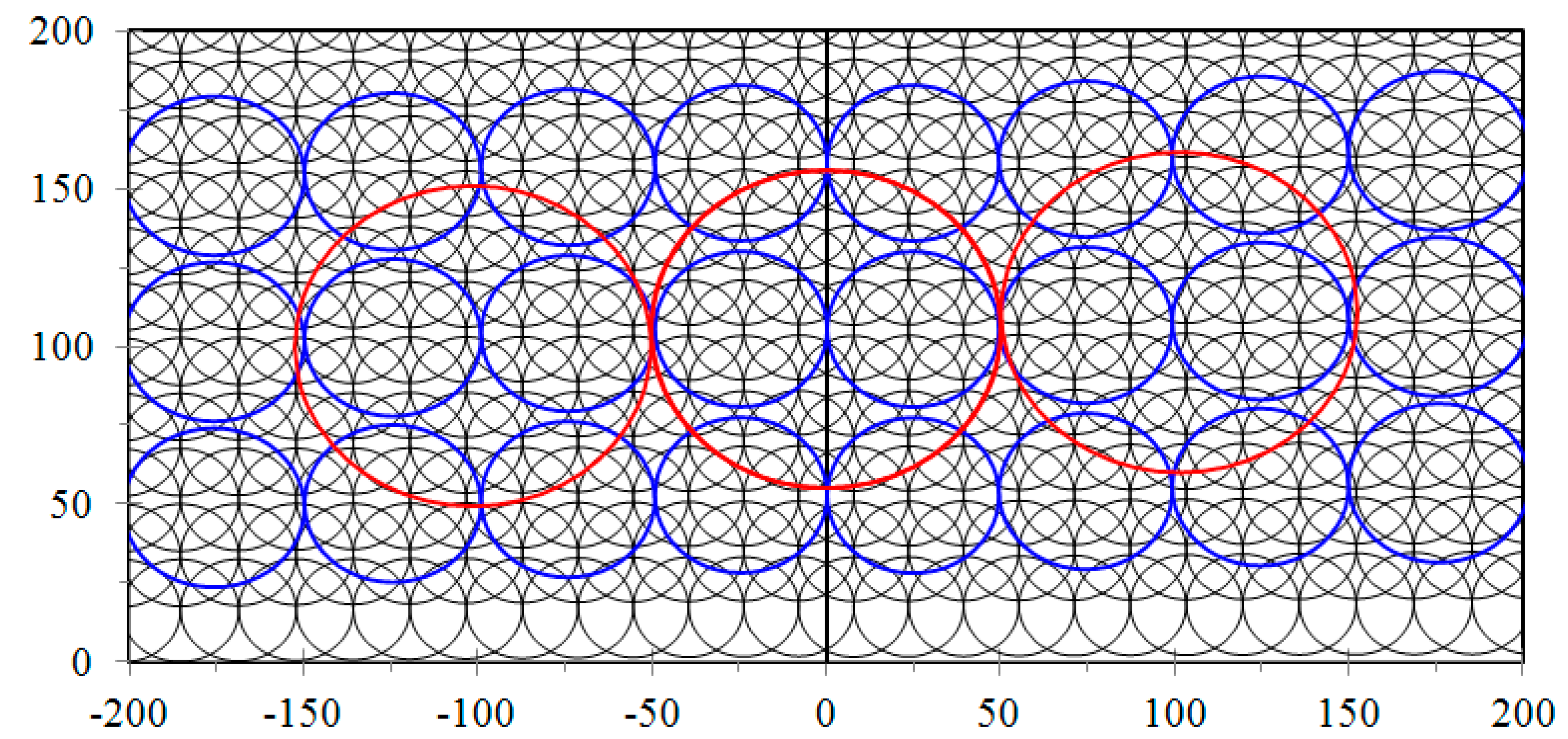
ATMS scan angle ranges within ±52.725° from the nadir direction and has 22 channels, with the first 16 channels primarily for temperature soundings from the surface to about 1 hPa (~45 km), and the remaining six channels for humidity soundings in the troposphere from the surface to about 200 hPa (~15 km). ATMS channels 3–16 have a beam width of 2.2°, which is smaller than that of corresponding AMSU-A channels 3–15 (see
Figure 1). However, the beam width of ATMS channels 1–2 is 5.2°, which is much larger than that of corresponding AMSU-A channels 1–2. ATMS channels 17–22 have a beam width of 1.1°, which is the same as that of the AMSU-B and MHS channels.
The ATMS scan mechanism is synchronized to the spacecraft clock, with a “sync” pulse every eight seconds (
i.e., at every third revolution). Each ATMS scan cycle is divided into three segments. In the first segment, the Earth is viewed at 96 different scan angles, which are distributed symmetrically around the nadir direction (see
Figure 1). The 96 ATMS field-of-view (FOV) samples are taken with each FOV sample representing the mid-point of a brief sampling interval of about 18 ms. With a scan rate of 61.6° per second, the angular sampling interval is 1.11°. Therefore, the angular range between the first and last (
i.e., 96th) sample centroids is 105.45° (
i.e., ±52.725° relative to the nadir). As soon as one scan line scan is completed, the antenna accelerates and moves to a position that points to an unobstructed view of space (
i.e., between the Earth
’s limb and the spacecraft horizon). Four consecutive cold calibration measurements are taken. Next, the antenna accelerates again to the zenith direction, where the blackbody target is located, and takes four consecutive warm calibration measurements with the same slow scan speed. Finally, it accelerates back to the starting position, resumes the same slow scan speed as it scans across the Earth scenes, and continues the next scan cycle.
Compared to its predecessors, AMSU-A/MHS (see
Table 1), three new ATMS channels (4, 18 and 19) were added to improve the profiling of atmospheric temperature and water vapor. Additionally, the polarization for ATMS channels 3 and 5 are also different from the corresponding AMSU-A channels. In higher elevation terrains, where these channels become surface sensitive, the polarization difference can result in a difference in brightness temperatures when the surface is specular. Note that ATMS channel 17 has a higher frequency than MHS channels and, thus, the scattering from atmospheric and surface medium may be slightly stronger, resulting in lower brightness temperatures.
ATMS has two sets of receiving antennas and reflectors. One serves channels 1–15, with frequencies below 60 GHz, and the other serves channels 16–22, with frequencies above 60 GHz. Each receiving antenna is paired with a plane reflector mounted on a scan axis at a 45° tilt angle so that the incoming radiation is reflected from a direction perpendicular to the scan axis into a direction along the scan axis (i.e., a 90° reflection). The scan axis oriented in the along-track direction results in a cross-track scan pattern. The reflected radiation is focused by a stationary parabolic reflector onto a dichroic plate, and then either reflected to or passed through to a feedhorn. Each aperture/reflector serves two frequency bands for a total of four bands.
3. ATMS Calibration Error Budget Model
Calibration measurements are used to accurately determine the so-called radiometer transfer function that relates the measured digitized output (
i.e., counts) to a radiometric brightness temperature. The ATMS radiometric calibration for antenna brightness temperature is derived as follows:
where
and
are the radiance of warm and cold calibration targets corresponding to the warm and cold target temperatures (
and
), respectively;
and
are the mean warm and cold counts within the calibration window, respectively;
is the scene count; and
is the calibration non-linearity term [
13,
14]
where
is nonlinearity parameters and sensitive to variation of instrument temperature. The non-linearity term can be also expressed in terms of the radiance ratio from the linear calibration,
i.e.,:
where:
where
is linear part of calibrated radiance. Assuming no error in measurement counts, the absolute calibration accuracy is expressed as:
or:
From Equation (6), we can see that the calibration accuracy is determined by radiance errors of warm and cold calibration targets ( and ) and the maximum nonlinearity ().
3.1. Errors from Warm Target Radiance Computation
The radiance of the warm target is dependent on the following three terms: warm load emissivity
, physical temperature
and external radiation
:
If the warm target is not a perfect blackbody, the emitted radiation is less than the value computed from the Planck function, resulting in a difference of:
where
is the physical temperature of a warm target measured from PRTs. For ATMS, its warm target effective emissivity is no less than 0.9999. Thus, at a temperature of 300 K, the resulting error in brightness temperature is no more than −0.03 K. The uncertainty of the warm target radiance,
, depends on temperature drifts, temperature gradients, and inaccurate temperature measurements. Temperature drift is the target temperature change between the time of radiometric observation and the time that the physical temperature is measured. For ATMS, the maximum time delay is 2.67 s (the scan period), and the maximum thermal drift rate is about 0.001 K/s. Thermal analyses indicate that the maximum rate, which occurs at the eclipse in a beta angle (angle between sun vector and orbit plane) of 80 degrees orbit, will be no greater than this requirement. In the actual ATMS design, the physical temperature measurements are centered at the same time as the warm calibration radiometric measurements. Therefore, for the nominal-case error budget, this item is reduced to a negligible contribution. The temperature spatial gradient of the warm target is no greater than 0.05 K. The use of multiple temperature sensors allows for an averaging that reduces horizontal gradients. However, the vertical gradients still exist and will contribute directly to the calibration error. The vertical gradients are a function of the horizontal position on the pyramidal tines, and the effect on calibration error will be the temperature error averaged over the horizontal plane.
The temperature measurement accuracy pertains to the accuracy of the Platinum Resistance Temperature sensors (PRTs) and their associated read-out electronics. The single four-wire PRT accuracy is about 0.10 K. The averaging of readings from seven PRTs (minimum required for each calibration target) will reduce the error, but the reduction factor is largely unknown since some of the error terms may be partially correlated. The resulting end-of-life (EOL) value for a single PRT is therefore used for the error budget study.
The external radiation is caused by the imperfect coupling of the reflector/shroud assembly to the warm load. The error due to this coupling is given by:
where
is the coupling factor, and
and
are the radiance of warm load and external environment, respectively. The worst-case condition is when the warm load is heated to a maximum and the external environment is at a minimum. Thermal analyses indicate that the maximum target temperature is 330 K. The environment, facing the Earth, with reflective obstructions on all sides, is approximated as a 75% view of Earth and 25% view of cold space. At a minimum Earth brightness temperature of 150 K, this gives a radiance error in terms of brightness temperature of 0.2 K.
3.2. Errors from Cold Space Radiance Computation
Uncertainties in the radiance of the cold target observation are dependent upon the Earth contamination through antenna sidelobes (
), the spacecraft contamination through antenna sidelobes (
), and the uncertainty of the actual cosmic radiation (
),
i.e.,:
For the nominal-case error budget, the actual predicted antenna sidelobe levels were used to predict the error contributions from the Earth and spacecraft intercepts. The first calculation involves integration of a worst-case ATMS far-field antenna pattern over the angular region subtended by the Earth for the primary cold calibration beam position at a spacecraft altitude of 833 km. Both co- and cross-polarized antenna patterns were employed in the computations because the rotation of the reflector with respect to the feedhorn causes a rotation of the incident vertical and horizontal polarization. The second calculation involved an integration of the near-field energy density of the antenna over regions of the spacecraft structures to determine the fraction of energy received from spacecraft reflections of Earth radiation. This was done both for the cases of maximally allowed spacecraft intrusions into the cold space hemisphere and for an expected typical case based on proposed satellite configurations. For Suomi NPP ATMS, the cold target calibration error for the worse case is about 0.3 to 0.5 K from the Earth contamination and 0.08 to 0.13 K from the spacecraft contamination. When the calibration equation is performed in radiance space, the uncertainty in computing the cosmic radiance is determined by the cosmic temperature, which is 2.72548 K ± 0.00057 K [
15].
3.3. Errors from Nonlinearity Uncertainty
The error in calibration accuracy is also related to the non-linearity uncertainty,
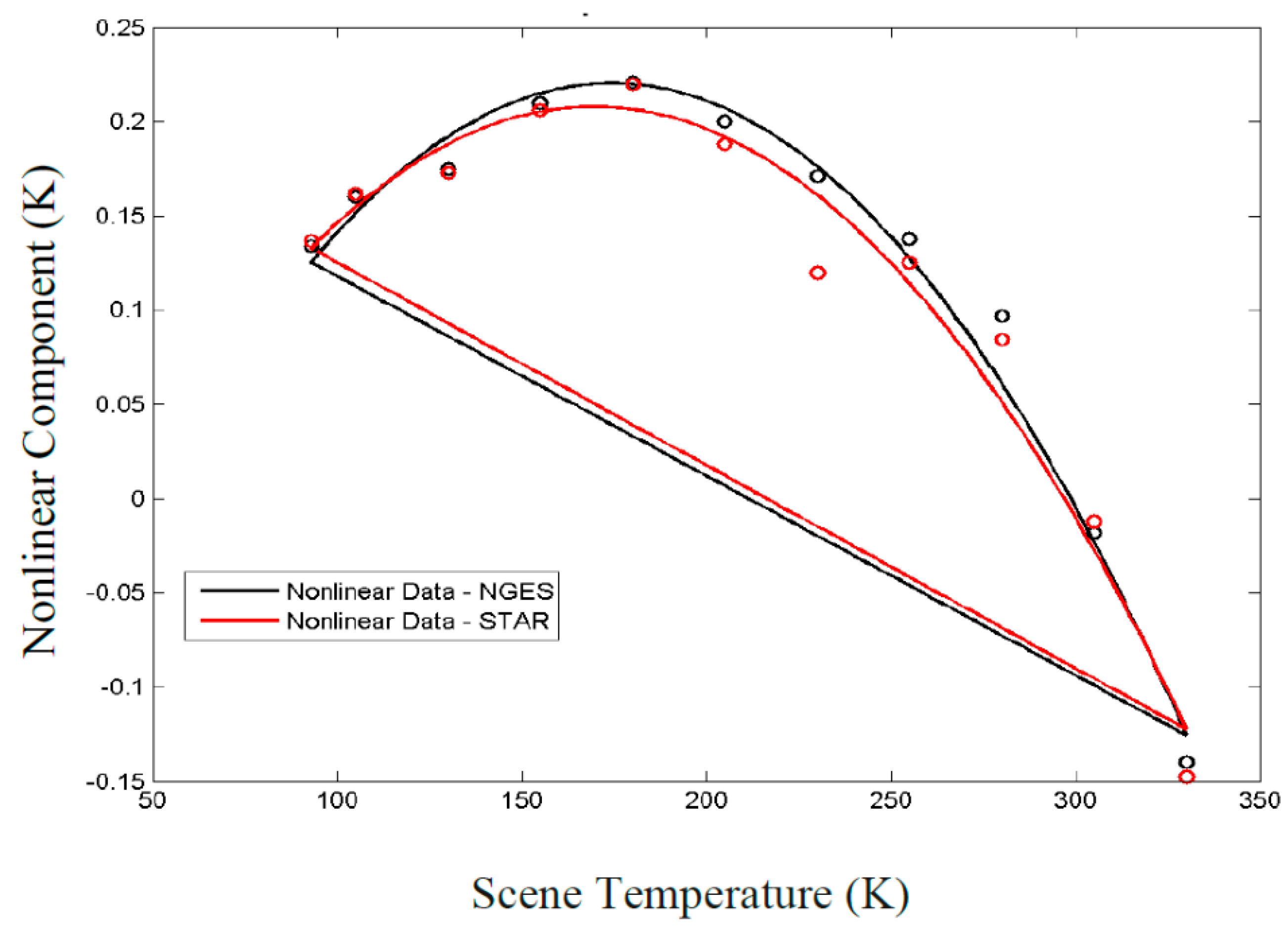
. For the thermal channels, nonlinearity is derived during the prelaunch phase through the thermal vacuum chamber (TVAC) data. The scene targets are controllable to establish 11 temperatures ranging from 95 K to 330 K, and the cold targets were set to a nominal of 95 K. These tests were carried out at three different instrument temperatures, 8 °C, 20 °C and −5 °C, to simulate the possible on-orbit temperature variation the instrument may undergo. The radiometric accuracy is computed as the difference between the brightness temperature inferred from radiometric counts, and the physical temperature of the scene target as derived from PRT measurements. The nonlinearity was calculated as the difference between the measured scene radiance and the linear term in Equation (6), which is:
The maximum nonlinearity is determined at a mid-point of scene temperature ranging from 95 K to 330 K (see
Figure 2). The on-orbit nonlinearity can be predicted by performing a quadratic curve fitting to calibration accuracy (which is defined as the difference between linear calibrated scene radiance and the scene truth from PRTs measurements) derived from two-point calibration of TVAC data and extrapolating to 2.728 K of cold space temperature, the maximum nonlinearity can be found by taking the difference between the fitting curve and the line connecting 2.728 K and 330 K temperature point. For Suomi ATMS, the peak non-linearity, over the dynamic range of 3 to 300 K, is 0.278 K for channel 1, and 0.384 K for channels 2–22. These values are used for the worst-case budget. The nominal-case budget uses values derived from component-level performance predictions.
3.4. Calibration Accuracy for SNPP ATMS Prototype Flight Model
The ATMS Prototype Flight Model (PFM) test data that are used for predicting on-orbit calibration accuracy are shown in
Table 2. The target external coupling loss is calculated from the nominal coupling factors for the target temperature of 265 K. The cold calibration errors due to sidelobe Earth intercept were derived from antenna pattern measurements. The peak non-linearity was derived from system Thermal Vacuum Calibration data by computing quadratic regression curves extrapolated to the on-orbit cold calibration temperature.
Table 3,
Table 4 and
Table 5 show the resulting performance predictions using these PFM measured parameters for three cases of low (80 K), mid (190 K), and high (300 K) scene temperatures. Notice that ATMS has six redundant configuration (RC) electronic units, but, in the operation, we only use the RC1. Overall, the calibration accuracy at all three scene temperatures meet the specifications, compared to the requirements. The magnitude ranges from 0.1 to 0.4 K. At the mid-scene temperature, the calibration errors seem to be generally higher than those at warm and cold scenes. Note that, for ATMS, the maximum nonlinearity typically occurs near the mid-scene temperature and its uncertainty may have the highest contribution to the increased calibration errors.
4. Verification of ATMS Calibration Accuracy through SNPP Pitch Maneuver Observations
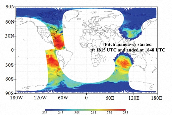
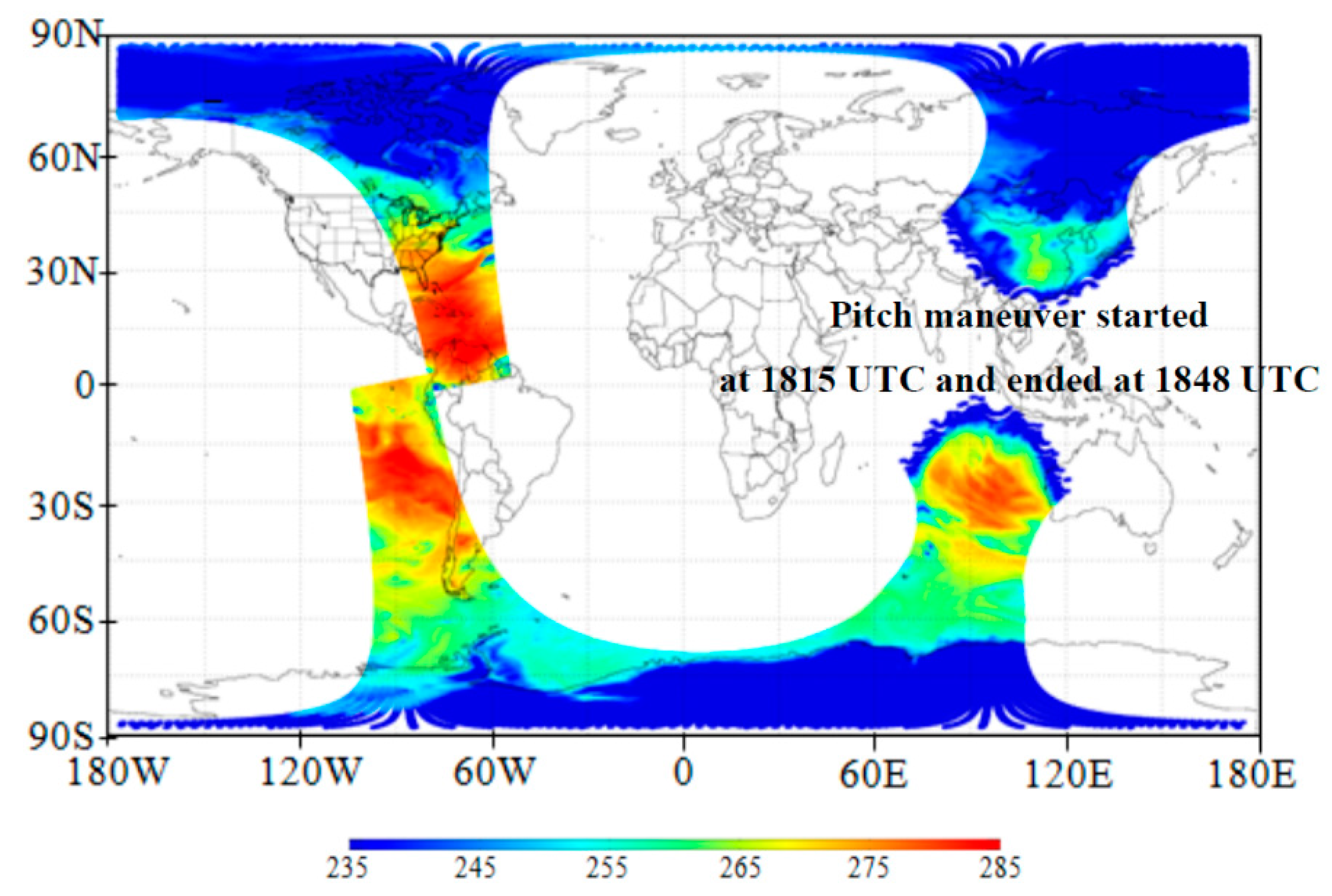
On 18 February, 2012, the Suomi NPP satellite was commanded to look over cold space. For ATMS, this maneuver establishes a baseline radiometer output from pure cold space. As shown in
Figure 3, the maneuver started at 1815 UTC and ended at 1848 UTC in the descending orbit, and thus a large portion of this 33-min period is over oceans. The spacecraft is pitched completely off the Earth to enable all the instruments to acquire full scans of deep space, permitting the deviations from the uniformity of the field of view to be characterized. When the Earth
’s disk lies totally outside the scan direction, there should be good sensitivity for the all the instruments to see any anomalies introduced by obstacles near the spacecraft itself and radiation emitted from the ATMS scanning system and other instruments. For the SNPP mission, Earth is visible by the ATMS antenna at 62.37° (local zenith angle of 27.63°) from the nadir, assuming the Earth diameter is approximated 12,742 km. Since the ATMS cross scan swath is about 2600 km, complete ocean views are possible if the maneuver is performed over Indian, South Atlantic, North Atlantic, and Pacific Ocean regions.
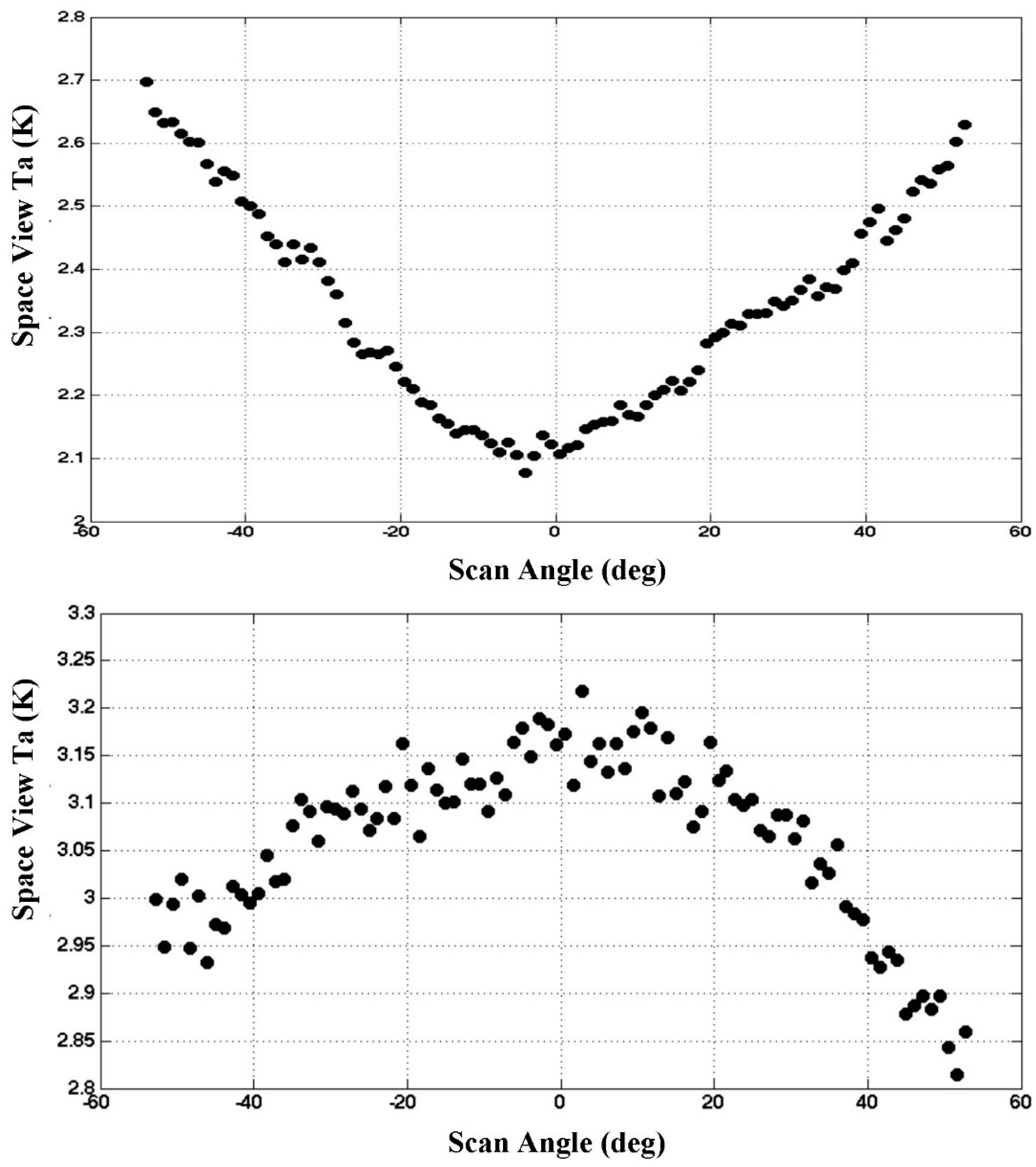
Figure 4 shows ATMS antenna brightness temperatures at channels 1 and 3 from all the data processed by the JPSS ground software (Algorithm Dynamic Library (ADL) version 5.11) in which a full radiance calibration is applied. Note that the data points at each scan position are averaged from all the observations between 1820 UTC to 1845 UTC when ATMS scans through space. From 96 field-of-views brightness temperatures, we selected three center positions, 46, 47, and 48, as approximations to the cosmic radiation at 2.728 K.
Table 6 lists the biases of the pitch maneuver brightness temperatures from 2.728 K for the 22 channels ATMS. The biases at channels 1, 2 and 16 are negative and those at the other channels are positive. The magnitude of bias exceeded those predicted by the PFM error budget model. It is also shown that the bias at each channel depends on scan angle. The patterns for quasi-vertical polarization at channels 1, 2, and 16 have a “smile” shape, whereas those for quasi-horizontal polarization have a “frown” shape. The bias at the nadir positions and the scan angle dependent bias can be well explained by the antenna emission model, which is discussed in details in the next section.
5. An Antenna Emission Model for Improving ATMS Calibration Accuracy
As shown in the previous section, a systematic scan-dependent radiometric bias was observed from a pitch-over maneuver. A homogeneous and un-polarized cold-space cross scan showed that this bias is a sine-squared function of scan angle for the Quasi-Vertical (QV) channels (channels 1, 2, 16), and a cosine-squared function of scan angle for the Quasi-Horizontal (QH) channels (channels 3–15, 17–22) [
10]. After examining the SNPP ATMS antenna pattern coefficients, we found that for pitch-over observations ATMS sidelobe coefficients at most of channels are very small and are generally less than 0.02%. Thus, the expected side-lobe contribution from the reflected solar and earth is insignificant [
14]. Additionally, since ATMS instrument is mounted on the side of the SNPP spacecraft, it should be a more asymmetric pattern if the side-lobe effect is dominating the scan angle dependent bias. However, in the deep space observations, the bias is more symmetric with cosine-square and sinusoidal-square functions. Polarization angle twist is an unlikely cause for this bias during the cold space observations since they are unpolarized and, thus, the sine- and cosine-weighted radiances do not change with any twisted angles.
The root cause that can be hypothesized and that explains these bias characteristics is the emissivity of the rotating flat plate reflector of the Scan Drive Mechanism (SDM). When viewing an emissive surface at a 45 degrees angle, the emissivity for the polarization component in the plane of incidence is greater than that for the component normal to the plane of incidence. When the rotating reflector is viewed by a stationary linear-polarized feedhorn, the resulting signal has a sinusoidal variation with scan angle. The facts that all QV channels have a sine-square function and all QH channels have a cosine-square function are exactly what can be explained by this theory.
According to the Hagen-Rubens equation [
16], the emissivity of a conducting surface, viewed at normal incidence, is:
where f is the receiver frequency and σ is the conductivity of the reflecting surface. This equation should be valid for perfectly smooth and pure bulk conductive materials. The actual emissivity of real reflector surfaces is invariably greater than the theoretical value due primarily to surface roughness and impurities. The SNPP ATMS flight reflector is made of Beryllium with a nominally 0.6 micron gold plating layer on a Nickel interfacing layer. Since the gold plating thickness is comparable to the skin depth, and is likely to have extreme microscopic granularity and roughness, it is expected that the emissivity would greatly exceed the values computed from the Hagen-Rubens equation. Estimates of the emissivity for the PFM flight unit based on the pitch-over maneuver were in the range from 0.0026 to 0.0063 over all the ATMS frequency bands [
17]. For comparison, the Hagen-Rubens equation gives an emissivity of about 0.0005 to 0.0014 for pure bulk gold over the range of 23 to 183 GHz. Thus, radiances for quasi-V and -H channels are derived as follows:
where
and
are the quasi-V and -H radiances from Equation (1), respectively.
and
are the QV and QH radiances contributed from the reflector emitted radiation, respectively.
,
and
are the radiative components at pure vertical and horizontal polarization, and the third Stokes component.
is the radiance emitted from reflector.
and
are the reflector emissivity at the vertical and horizontal polarization, respectively. At an incident angle of 45 degrees from the reflector normal:
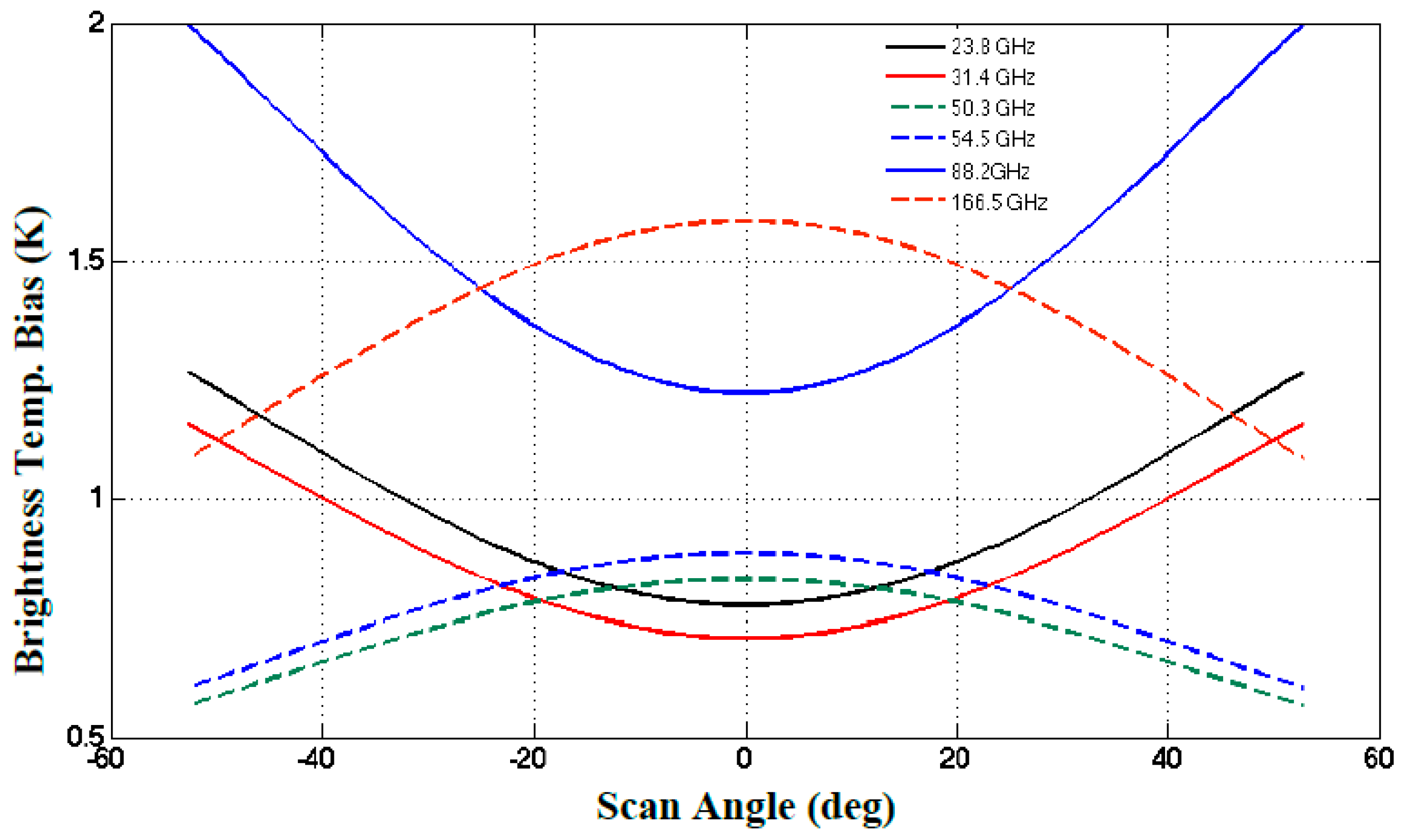
When ATMS views cold space, the biases due to the last three terms in Equation (13) are simulated as a function of scan angle and shown in
Figure 5. For QV channels, the bias at the center direction ranges from 0.3 to 1.3 K given its emissivity from 0.0028 to 0.0043 at the reflector temperature of 283 K. Additionally, the emission magnitude varies within 0.5 K from center to the limb, which is consistent with the ATMS cold space observations, as shown in
Figure 4. It is clearly seen that the impacts of reflector emissivity are dependent on polarization. For QV channels, it is a square of the sinusoidal curve and whereas for QH channels it follows a cosine curve. Additionally, the effects of reflector emission are the highest when the antenna views the cold cosmic background.
From Equation (13), we can first estimate the effects of the reflector emission on radiation from warm and cold calibration targets. When the antenna views the cold space calibration target at a scan angle of 81.69° and the warm calibration target at an angle of −163.34°, the additional radiation components contributed to the cold calibration are estimated and shown in
Table 7. It is quite clear that the corrections to the warm target brightness temperature are much smaller than those corrections made to the cold calibration. This is because the warm target temperature is operated at 300 K that is close to the antenna reflector temperature (
280 K). The uncertainty introduced by the antenna emission to the cosmic radiative temperature (2.728 K) is also dependent on frequency or channel. In particular, the magnitudes at quasi-vertical polarization channels (1, 2 and 16) are much larger than those at the quasi-horizontal polarization channels.
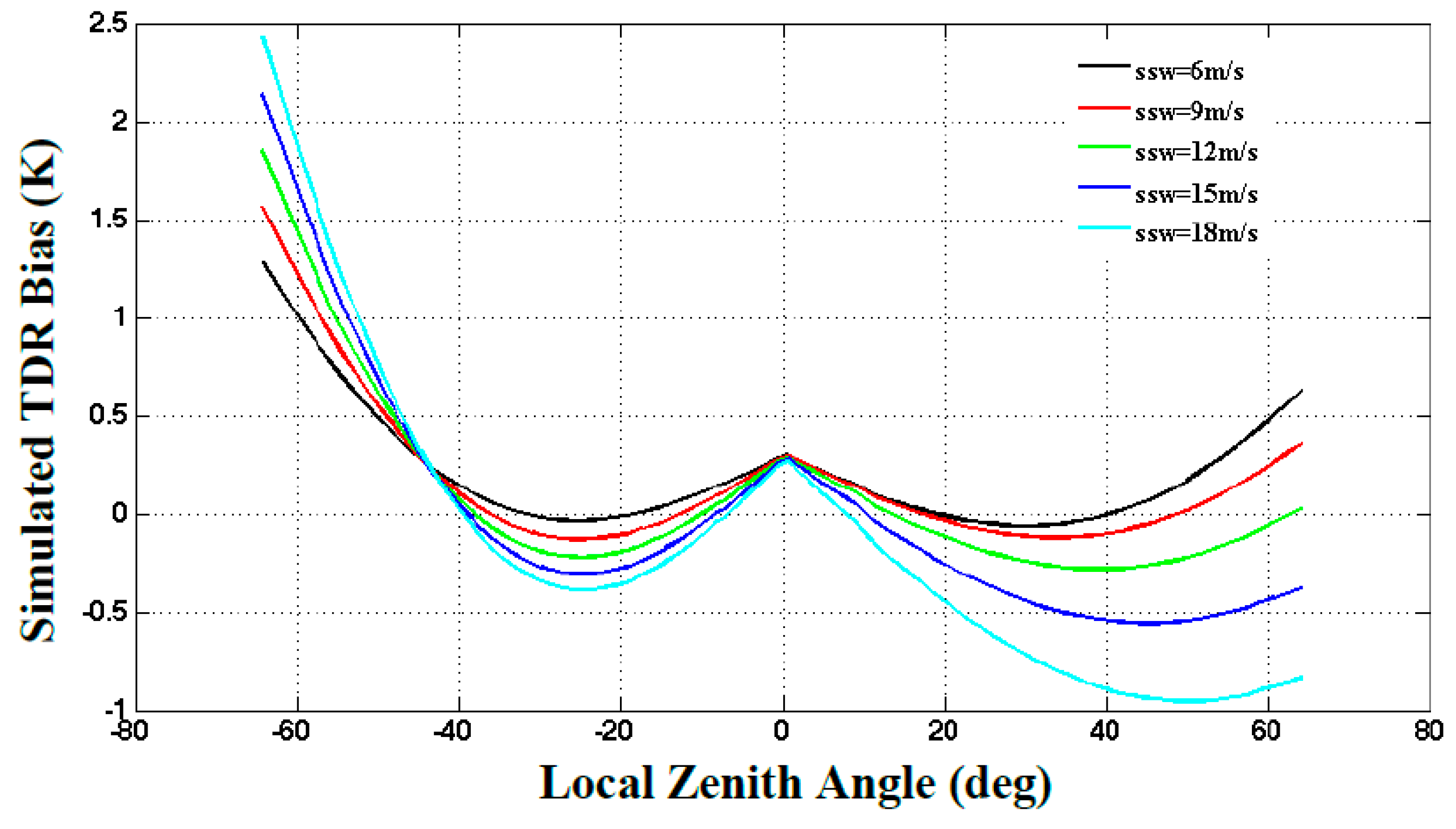
The implications from ATMS pitch maneuver data are several folds. Firstly, in the ATMS radiometric calibration, antenna reflector emission must be taken into account in the total radiation from two calibration targets. Secondly, when the ATMS antenna brightness temperatures are compared with theoretical simulations, a full polarimetric forward model that includes the third Stokes component should be utilized as shown Equation (13). If the polarization components in Equation (13) in the last three terms are neglected, the biases are pronounced. As shown in
Figure 6, the contributions from the third Stokes component can result in more asymmetric biases when the ocean wind speed increases from 6 to 18 m·s
−1. For example, for a wind speed of 15 m/s, the left to right asymmetry is about 0.5 K at a local zenith angle of 58 degree. Note that the simulations are made without considering the atmospheric effects on the radiative transfer.
6. Summary and Conclusions
ATMS is a spaceborne cross-track scanning total power microwave radiometer. Its radiometric counts are converted into the radiance from the two-point non-linear calibration equation. The warm target and cold space are two calibration sources and the accuracy in computing their radiances or brightness temperatures is affected by variable sources. The nonlinearity of the calibration equation is quantified from the prelaunch thermal vacuum data. In ATMS radiometric error budget model, the instrument calibration accuracy is primarily determined by the errors of warm target and cold space brightness temperatures, and calibration nonlinearity. It is shown from the error budget model that the Suomi NPP ATMS calibration accuracy meets the requirements with a significant margin.
While the ATMS calibration accuracy meets the requirements, substantial biases are found at all the channels when the ATMS was pitched over to scan the uniform cosmic background. Through our further analysis and improvements to calibration theory, we found the ATMS antenna plane reflector has small but non-negligible emission. The magnitude of the emission is dependent upon frequency, polarization and scene radiative temperature. For ATMS warm target, the correction due to the reflector emission is very small due to its physical temperature close to the reflector temperature. For the cold calibration target at a temperature of 2.728 K, the correction due to the reflector emission is significant. This correction should be implemented into the ATMS radiometric calibration to further improve the calibration accuracy. In doing so, three terms related to the reflector emissivity are added to the radiance or brightness temperatures of warm target and cold space. Additionally, a full polarimetric model is developed for computing the scene brightness temperatures and can be used for a comparison with ATMS observations.


