Estimating Stand Volume and Above-Ground Biomass of Urban Forests Using LiDAR

Abstract

Assessing forest stand conditions in urban and peri-urban areas is essential to support ecosystem service planning and management, as most of the ecosystem services provided are a consequence of forest stand characteristics. However, collecting data for assessing forest stand conditions is time consuming and labor intensive. A plausible approach for addressing this issue is to establish a relationship between in situ measurements of stand characteristics and data from airborne laser scanning (LiDAR). In this study we assessed forest stand volume and above-ground biomass (AGB) in a broadleaved urban forest, using a combination of LiDAR-derived metrics, which takes the form of a forest allometric model. We tested various methods for extracting proxies of basal area (BA) and mean stand height (H) from the LiDAR point-cloud distribution and evaluated the performance of different models in estimating forest stand volume and AGB. The best predictors for both models were the scale parameters of the Weibull distribution of all returns (except the first) (proxy of BA) and the 95th percentile of the distribution of all first returns (proxy of H). The R² were 0.81 (p < 0.01) for the stand volume model and 0.77 (p < 0.01) for the AGB model with a RMSE of 23.66 m³·ha⁻¹ (23.3%) and 19.59 Mg·ha⁻¹ (23.9%), respectively. We found that a combination of two LiDAR-derived variables (i.e., proxy of BA and proxy of H), which take the form of a forest allometric model, can be used to estimate stand volume and above-ground biomass in broadleaved urban forest areas. Our results can be compared to other studies conducted using LiDAR in broadleaved forests with similar methods.

1. Introduction

In recent decades, considerable amounts of afforestation and reforestation projects have been undertaken to address the increasing environmental issues related to climate change effects, urban sprawl, soil reclamation, soil sealing and degradation, biodiversity loss, water and air purification, etc., in most cities [1,2,3]. These “new” forests, namely urban forest plantations, are normally established over abandoned lands (e.g., former industrial sites) to enhance ecosystem services (ESS) for local communities [4,5]. These forests are established by cities to achieve their regulatory requirements for clean air, soil quality, and water management [6] while revitalizing livelihoods and human well-being [7,8].

ESS provided by urban forest plantations are assessed on the bases of forest stand characteristics, such as canopy height, stand density, stand volume, and biomass [9,10,11]. For example, Sandström et al. (2006) [12] reported a positive relationship between bird species richness, abundance and stand density in urban and peri-urban landscapes. However, such an assessment is often time consuming and expensive in terms of labor and costs for collecting field measurements of forest stands (e.g., tree diameter and height) [13]. An alternative approach would be to collect the necessary data using remote sensing technology through establishing empirical relationships between field measurements and spectral data. With the rapid development of computing and remote sensing technology, active sensors, such as Light Detection and Ranging (LiDAR), have emerged as promising tools [14,15,16]. LiDAR-based applications have expanded rapidly in the past two decades to model leaf distribution [17], 3-D canopy structure [18], spatial distributions of trees and canopies in complex topography [19,20], as well as species diversity [21,22,23,24]. For example, Omasa et al. (2008) used airborne and portable laser scanners to estimate the height of individual trees in Tokyo, Japan [25]. Shrestha et al. (2012) estimated the above-ground biomass of an urban forest in Oklahoma, USA, using the 95th percentile of the LiDAR point-cloud distribution [26] (see also Huang et al. 2013 [27]). Regardless of the growing body of literature on LiDAR applications in urban landscapes, the effective predictors (i.e., LiDAR-derived variables) of forest stand characteristics remain challenging because the large variations among forests and landscapes. Substantially more effort is needed to establish LiDAR-based models that are both cost-effective and suitable for sound estimations of tree allometry in different urban forest plantations.

In this study we assessed forest stand volume (VOL) and above-ground biomass (AGB) in an urban forest area located in Northern Italy. We selected two variables derived from the LiDAR point cloud distribution and combined them into a general forest allometric model, which takes the following form:

$$Y={\mathsf{\beta }}_0{(B{A}_{proxy})}^{{\mathsf{\beta }}_1}{(H_{proxy})}^{{\mathsf{\beta }}_2}$$

(1)

where, Y represents a given forest stand characteristic, such as stand volume or above-ground biomass; BA_proxy and H_proxy are the LiDAR-derived variables representing, respectively, forest stand basal area (BA) and mean tree height (H).

We tested various methods for extracting proxies of BA and H from the LiDAR point-cloud distribution and assessed the performance of different models estimating forest stand characteristics. The best models were validated using a Leave-One-Out Cross-Validation (LOOCV) method. If successful, our investigation will be an essential step for assessing the ESS provided by urban forest plantations (e.g., carbon storage).

2. Materials and Methods

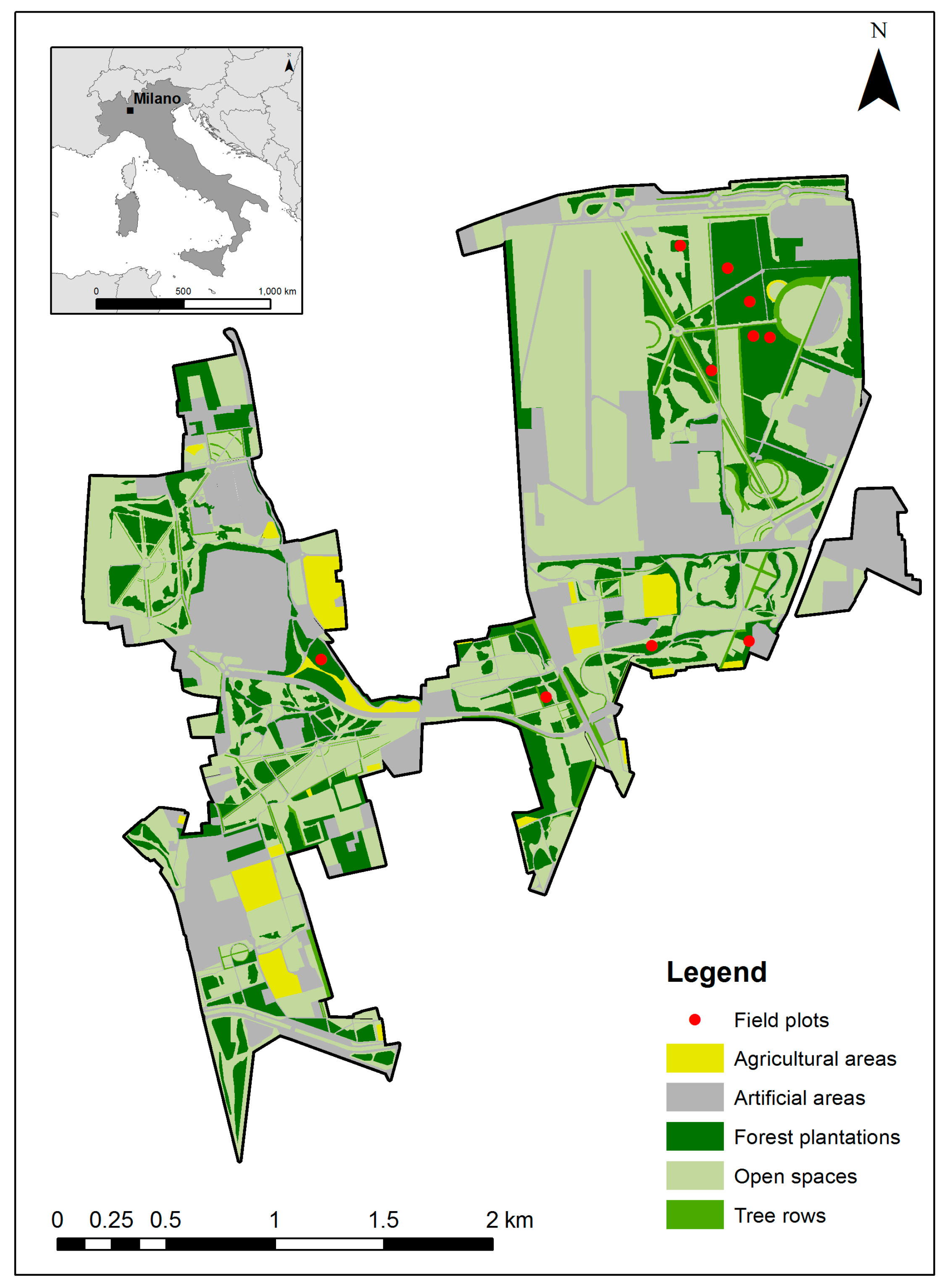
2.1. Study Area and Stand Delineation

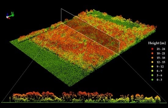
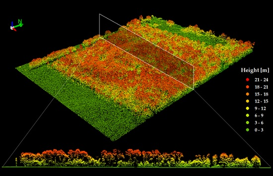
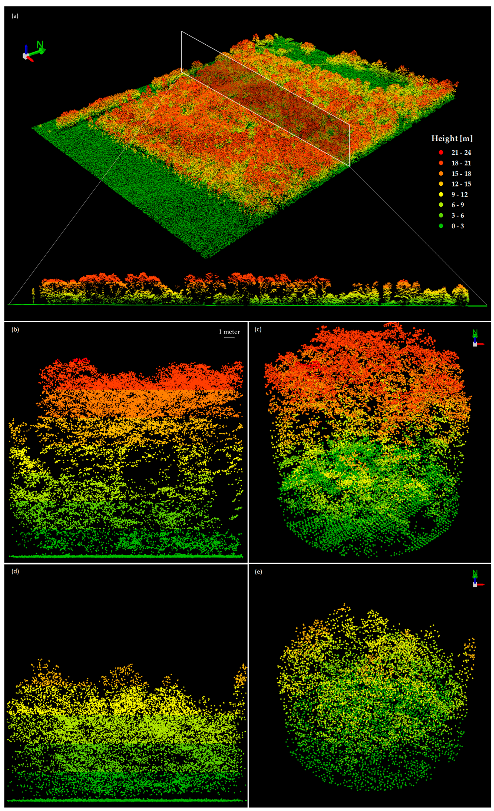
We based our study in an urban forest plantation located in the metropolitan area of Milan, Northern Italy: Parco Nord Milano (PNM) (45°53’71”N, 9°20’7”E). The entire area covers ~600 ha, with 100 ha as forest plantation and the remaining area as green space (e.g., tree rows, agricultural areas) and other recreational facilities or artificial areas (e.g., sports fields). PNM was established in the early 1980s as the result of a large afforestation plan supported by local authorities. Almost all of the trees are broadleaved. The vegetation, microclimate, and soil characteristics of the study area have been well documented by Sanesi et al. (2007) [28] and Marziliano et al. (2013) [10].

We collected quantitative measurements of the forest in PNM at 10 sample plots of 13 m radius (~500 m²) in September 2012 (Figure 1). The field plots were selected to represent the variety of species that were used in PNM upon its establishment (1983), e.g., Acer spp., Carpinus betulus, Fraxinus spp., Prunus avium, Quercus cerris, Quercus robur, Tilia spp., and Ulmus spp. (for more details see Marziliano et al. 2013; [10]). Moreover, plots were selected to represent three stages of forest stand development (i.e., stand age class): (1) <17 year; (2) 18–25 years; and (3) >25 years. Within each plot, all trees with a diameter equal or greater than 10 cm were identified by species and measured for their diameter at breast height (DBH), height, crown width at four cardinal directions, and crown depth (Figure S1). Field survey was undertaken using a Trimble GeoXT 6000 GPS. The GPS receiver had an estimated sub-meter accuracy after differential correction. From these measurements, we calculated the plot-level BA, mean DBH, and mean H. Stand VOL and AGB were calculated using the allometric equations of the Italian National Forest Inventory system [29]. For each tree, the following allometric equation was used:

$$Yi={\mathsf{\beta }}_0+{\mathsf{\beta }}_{1}DB{H_i}^{2}H+{\mathsf{\beta }}_{2}DB{H}_i$$

(2)

were Y_i is the forest stand characteristic for a tree (AGB or VOL), DBH_i and H_i are, respectively, the height and the diameter at breast height of the given tree. For each plot, total VOL and AGB were calculated by summing the values of all the trees belonging to the plot.

2.2. LiDAR Data

Airborne LiDAR data were acquired on September 2012, using an LMS-Q680i scanner (RIEGL). Extraction of the discrete points was conducted by the provider with the standard Riegl processing procedures. The average point density was 10 points/m², with a maximum of seven returns per impulse. This results in a relative position accuracy of ±10 cm and a relative height accuracy of ±7 cm (see

Table 1. Characteristics of the Airborne LiDAR scanner and flight specification of the acquisition survey conducted for this study.

Characteristic	Specifications
Laser scanner	Riegl LMS-Q680i
Point density	±10/m2
Laser pulse rate	290 kHz
Wavelength	Near infrared
Position accuracy	±10 cm
Height accuracy	±7 cm
Field of View	60°
Number of returns	≤7

). All the points with a scan angle greater than 10 degrees were excluded from the processing (Figure 2). After excluding the points, the average point density was 6 points/m².

LiDAR point-cloud data were classified into ground and non-ground following Axelsson (2000) using Terrascan (Terrasolid Ltd., Helsinki, Finland). Our data processing was carried out with ERDAS Imagine 2014 (Hexagon Geospatial). From the non-ground point cloud, we extracted those points located only in the forest areas using a detailed land-cover map derived from aerial photographs (resolution = 0.30 m). For ground surface, we generated a Digital Terrain Model (DTM), at 1 × 1 m resolution, using an Inverse Distance Weighting interpolation. We scrutinized the quality of the DTM using 16 ground control points from our previous topographic survey. The mean error was 0.11 m, with a standard deviation of 0.15 m. Given the relatively flat topography of the study area, we considered the DTM sufficiently accurate. The DTM was used to calculate the relative height above-ground of the point cloud by subtracting the corresponding DTM height from each point. For each field-plot, a circular buffer with a radius of 12.7 m was created. The total number of LiDAR points for each plot were extracted and converted to ASCII files using the LAS tools (Rapidlasso, GmbH). The ASCII files were analyzed in R 3.1.3 (R development Core Team) [30]. Points with a height value less than 2 m were excluded from the dataset in order to reduce the effect of stones, shrubs and low vegetation which were not included in the present study [31].

2.3. LiDAR-Derived Basal Area (BA)

We assumed that BA is related to the tree height distribution of all LiDAR points except the first returns. By excluding the first returns (i.e., canopy layer), we omit the canopy layer from our analysis. For each field plot, we analyzed the frequency distribution (Figure 3) of the point cloud by testing two different methods: (1) Weibull probability density function and (2) area of the frequency histogram in different percentile intervals.

Several studies demonstrated that Weibull distribution is a reliable function for modeling the diameter’s distribution in various even-aged forest stands of coniferous and/or broadleaved species [32,33,34]. In this context, the “scale” parameter of the Weibull distribution appears to be related to the median diameter of the forest stand, while the “shape” parameter represents the skewness of the distribution [35]. For each plot, we fitted a two-parameter Weibull distribution function using the Broyden–Fletcher–Goldfarb–Shanno optimization algorithm available within the R package “MASS” [36]. The goodness of fit was evaluated with the mean square error (MSE):

$$MSE=\frac{1}{n}{\displaystyle \sum }_{i=i}^n{\left({\widehat{Y}}_i-Y_i\right)}^2$$

(3)

where, ${\widehat{Y}}_i$ and $Y_i$ are, respectively, the theoretical and observed values of the probability density estimated at 0.5 m intervals. The normalized mean square error (MSEn) was calculated after normalizing the MSE by the means of the fitted and empirical distributions.

We also calculated the area of the frequency histogram of the point-cloud distribution within a range of intervals: from the minimum height (i.e., 2 meters) to the 10th (A_nofirst0_10), 20th (A_nofirst0_20), 30th (A_nofirst0_30), 40th (A_nofirst0_40), 50th (A_nofirst0_50), 60th (A_nofirst0_60) and 70th percentile (A_nofirst0_70).

2.4. LiDAR-Derived Mean Stand Height

The first returns of LiDAR represent the top of the canopy layer. Consequently, we analyzed the distribution of these points to extract a proxy of the mean stand height (Figure 3). This was done by using two different methods: (1) percentile of the distribution, i.e., 90th (Perc_first90), 95th (Perc_first95) and 99th (Perc_first99) percentiles; and (2) area of the frequency histogram, i.e., from the 80th to the 90th percentile (A_first80_90), from the 80th to the 99th percentile (A_first80_99), from the 90th to the 95th percentile (A_first90_95), from the 90th to the 99th percentile (A_first90_99), and from the 95th to the 99th percentile (A_first95_99).

2.5. Model Development

We developed our empirical models starting from the general equation (Equation (1)) and selected the best-supported models estimating VOL and AGB. In each model, we considered two LiDAR-derived variables as proxies of basal area and mean stand height. We also tested the influence on the model performance of the interaction term (BA × H). Model parameters were calculated using the logarithmic form [14,37,38]:

$$\ln VOL={\mathsf{\beta }}_0+{\mathsf{\beta }}_1\text{ln}(B{A}_{proxy})+{\mathsf{\beta }}_2\text{ln}(H_{proxy})$$

(4)

$$\ln AGB={\mathsf{\beta }}_0+{\mathsf{\beta }}_1\text{ln}(B{A}_{proxy})+{\mathsf{\beta }}_2\text{ln}(H_{proxy})$$

(5)

where, BA_proxy is one of the LiDAR-derived variables for basal area (e.g., Weibull scale) and H_proxy is one of the LiDAR-derived variables for mean stand height (e.g., Perc_first90). The back-conversion to the multiplicative form introduces a bias that was corrected by adding half of the residual variance to the intercept before conversion [39]. The best-supported models were selected on the basis of the AIC (Akaike’s information criterion) value.

Each of the selected models was validated using the LOOCV procedure due to the limited number of sample plots. This procedure involves several iterative steps; for each step one of the observations was excluded from the model development. The resulting equation is then used to predict the response variable(s) for the excluded observation. A root mean square error of cross-validation (RMSEcv) was calculated at the end of the procedure and compared to the standard error of the regression (i.e., RMSE). The LOOCV procedure was performed using the DAAG R package [40].

3. Results

3.1. Basal Area (BA)

The scale parameter of the Weibull distributions for all LiDAR points, except the first returns (wb_nofirst), varied from 5.47 to 11.77, with a mean value of 8.36 and standard deviation (SD) of 2.08 (Figure 4). We tested the relationship between wb_nofirst and ground measurements with correlation analysis. The wb_nofirst values were highly related to field measurements of BA (Pearson = 0.78) and DBH (Pearson = 0.81) (

Table 2. Pearson correlation coefficient between LiDAR derived variables and ground measurements. BA is basal area; DBH is mean diameter at breast height; H is Height mean; A_nofirst0_10, A_nofirst0_20, A_nofirst0_30, A_nofirst0_40, A_nofirst0_50, A_nofirst0_60 and A_nofirst0_70 are the areas calculated from the height distribution of the LiDAR points of all returns except the first between 0 and the 10th percentile, 0 and the 20th percentile, 0 and the 30th percentile, 0 and the 40th percentile, 0 and the 50th percentile, 0 and the 60th percentile and 0 and the 70th percentile, respectively; A_first80_90, A_first80_99, A_first90_95, A_first90_99, A_first95_99 are the areas calculated from the height distribution of the LiDAR points belonging to the first return between the 80th and the 90th percentile; the 80th and the 99th percentile, the 90th and the 95th percentile, the 90th and the 99th percentile and the 95th and the 99th percentile, respectively.

LiDAR Derived Variables	Forest Stand Measurements
	BA	DBH
wbnofirst	0.78	0.81
Anofirst0_10	0.23	−0.08
Anofirst0_20	0.39	0.13
Anofirst0_30	0.38	0.08
Anofirst0_40	0.36	0.08
Anofirst0_50	0.33	0.05
Anofirst0_60	0.33	0.05
Anofirst0_70	0.36	0.09
	H
Afirst80_90	−0.36
Afirst80_95	−0.47
Afirst80_99	−0.51
Afirst90_95	−0.57
Afirst90_99	−0.68
Afirst95_99	−0.62
Percfirst90	0.92
Percfirst95	0.91
Percfirst99	0.89

). The MSEn of each Weibull distribution ranged from 6% to 32%, with the lowest MSEn found in the youngest plot, which were aged 12 years since plantation. The highest MSEn was found in one of the oldest plots (1A; 29 years old). Overall, the MSEn was lower in the five plots that were <25 years old (6.94%, 13.18%, 13.41%, 15.27%, and 15.82%) than the five plots of ≥25 years old (20.92%, 27.18%, 25.27%, 32.71%, and 23.7%). This is likely due to the characteristics of the height distributions that appeared to be bimodal as forests age increased.

We also analyzed the relationship between the area of the frequency histogram of the point-cloud distribution and ground measurements of BA (range: A_nofirst0_10, Pearson = 0.23; A_nofirst0_20, Pearson = 0.39) and DBH (range: A_nofirst0_50, Pearson = 0.05; A_nofirst0_60, Pearson = 0.13) (Table 2). In this case, correlation coefficients were significantly lower compared to the ones derived from the Weibull distribution.

3.2. Mean Stand Height

We tested the relationship between the LiDAR-derived variables collected from the top of the canopy layer (i.e., height distribution of the first returns) and ground measurements of the mean stand height (H): Perc_first90, Perc_first95 and Perc_first99 were highly correlated with the mean stand height (Pearson > 0.89) (Table 2). As for the relationship between the area of the frequency histogram of the point-cloud distribution (i.e., the first returns) and H, the Pearson coefficients ranged from −0.36 (A_first80_90) to −0.68 (A_first90_99). Considering that the purpose of the study was to select a LiDAR-based variable as a proxy of mean stand height, which is positively correlated with VOL and AGB, we did not include the variables associated with the area of the frequency histogram for mean stand height in our final models.

3.3. Model Selection and Validation

We selected the best-supported models explaining VOL and AGB from the 48 models (8 proxies of BA × 3 proxies of H × 2 presence/absence interaction term) generated from all combinations of the LiDAR-derived variables (Figure 5). The R² ranged from 0.72 to 0.84 (

Table 3. R², Akaike information criterion (AIC), Root mean square error (RMSE) and Root mean square error from cross validation (RMSEcv) of the best models for selected models. RMSE is expressed in m³·ha⁻¹ for forest stand volume (VOL) and in (Mg·ha⁻¹) for above-ground biomass (AGB). (i) Indicates the presence of an interaction term and bold characters indicates the best models.

Response Variable	Model	R2	AIC	RMSE	RMSEcv
ln VOL (m3·ha−1)	ln wbnofirst + ln Percfirst95	0.81	4.59	23.66 (23.3%)	32.86 (32.3%)
	ln Anofirst0_10 + ln Percfirst90	0.76	6.81	26.19 (25.7%)	35.64 (35%)
	ln wbnofirst + ln Percfirst95 (i)	0.81	6.58	23.67 (23.3%)	34.1 (33.5%)
	ln Anofirst0_20 + ln Percfirst95 (i)	0.84	4.71	20.18 (19.8%)	33.9 (33.3%)
ln AGB (Mg·ha−1)	ln wbnofirst + ln Percfirst95	0.77	4.8	19.59 (23.9%)	26.89 (32.9%)
	ln Anofirst0_10 + ln Percfirst90	0.72	6.81	21.52 (26.3%)	28.76 (35.1%)
	ln wbnofirst + ln Percfirst95 (i)	0.77	6.79	19.63 (24%)	27.81 (34%)
	ln Anofirst0_20 + ln Percfirst95 (i)	0.80	5.31	17.97 (22%)	31.11 (38%)

). In general, models estimating VOL performed better than those estimating AGB. The lower performance of the AGB model is probably due to the presence of different tree species and consequently different wood densities, which are not delectable from LiDAR. The inclusion of the interaction term slightly increased the R² and AIC. Given the low degrees of freedom available for the analysis (n = 10), we selected the best models using the AIC to reduce overfitting effects. Therefore, models with the interaction term were not included in the final selection.

The selected model forms are (

Table 4. Selected models with estimated coefficients for predicting stand volume (VOL) and above-ground biomass (AGB).

Response Variable	Model	β0	β1	β2
lnVOL	${\mathsf{\beta }}_0+{\mathsf{\beta }}_1\ln \left({\text{wb}}_{\text{nofirst}}\right)+{\mathsf{\beta }}_2\text{ln}\left({\text{Perc}}_{\text{first}}95\right)$	0.38	1.49	0.37
lnAGB	${\mathsf{\beta }}_0+{\mathsf{\beta }}_1\text{ln}\left({\text{wb}}_{\text{nofirst}}\right)+{\mathsf{\beta }}_2\text{ln}\left({\text{Perc}}_{\text{first}}95\right)$	0.78	1.44	0.19

):

$$\ln VOL={\mathsf{\beta }}_0+{\mathsf{\beta }}_{1}ln\left(w{b}_{nofirst}\right) +{\mathsf{\beta }}_2\text{ln}\left(Per{c}_{first}95\right)$$

(6)

$$\ln AGB={\mathsf{\beta }}_0+{\mathsf{\beta }}_{1}ln\left(w{b}_{nofirst}\right) +{\mathsf{\beta }}_2\text{ln}\left(Per{c}_{first}95\right)$$

(7)

where, wb_nofirst is the “scale” parameter of the Weibull distribution fitted on all LiDAR points except the first returns; Perc_first95 is the 95th percentile of the height distribution of LiDAR first returns. Both models were back-converted into their multiplicative form by adding half of the residual variance to the intercept (0.0297 and 0.030, respectively):

$$VOL=1.50*w{b}_{nofirst}^{1.49}*Per{c}_{first}{95}^{0.37}$$

(8)

$$AGB=2.52*w{b}_{nofirst}^{1.44}*Per{c}_{first}{95}^{0.19}$$

(9)

the R² was 0.81 (p = 0.001383) for the VOL model and 0.77 (p = 0.001988) for the AGB model; the AIC was 4.59 and 4.8, respectively (Figure 6). The two models were then validated using the LOOCV procedure. The RMSE of the VOL model was 23.66 m³·ha⁻¹ (23.3%) and the RMSEcv was 32.86 m³·ha⁻¹ (32.3%). The RMSE of the AGB model was 19.59 Mg·ha⁻¹ (23.9%) and the RMSEcv was 26.89 Mg·ha⁻¹ (32.9%). For both VOL and AGB models, the close match between RMSEcv and RMSE suggested that the regressions had good predictive powers and that the models were not overfitting [41,42].

With these models, VOL increased by approx. 1.5% when wb_nofirst increased by 1% and VOL increased by approx. 0.4% when Perc_first95 increased by 1%. Similarly, in the AGB model, AGB increased by approx. 1.4% when wb_nofirst increased by 1% and AGB increased by approx. 0.3% when Perc_first95 increased by 1%. Similar ratios between coefficients can be found in forest allometric models based on field data measurements [43,44,45].

4. Discussion

Modeling VOL and AGB using LiDAR-derived variables as proxies of forest measurements owes a large potential for future applications in forestry science, especially in urban forestry. For example, LiDAR-based applications can be used in connection with urban forest inventories, to derive information about the amount of carbon stored in the above-ground biomass (i.e., ecosystem service). Here, we provided a method for extracting LiDAR-derived variables from the point-cloud distribution and developed two models that take the form of a general forest allometric model to estimate stand volume and above-ground biomass of an urban forest.

In selecting the best model, a generalization was preferred toward model accuracy as this allows for broader application. Our findings are comparable with the outcomes of the other studies using LiDAR in broadleaved forests. For example, Lefsky et al. (1999) estimated AGB of a deciduous forest in Eastern Maryland (USA) using measurements of forest vertical structures derived from a full-wave LiDAR sensor with a coefficient of determination of 0.81 and an RMSE of 45.8 Mg·ha⁻¹ (19.2% of the mean) [46]. Popescu et al. (2004) used a tree-based approach to estimate stand volume and AGB in a deciduous forest in Virginia (USA), obtaining an R² of 0.39 (RMSE 52.84 Mg·ha⁻¹) and 0.32 (RMSE 44 m³·ha⁻¹) for stand volume and AGB, respectively [47]. More recently, Ioki et al. (2010) used an area based approach to estimate stand volume in an urban forest with an R² of 0.75 and an RMSE of 41.90 m³·ha⁻¹ (16.4% of the mean) [48].

Limitations of this study include the biases in the Weibull distribution fitting for the calculation of the LiDAR-derived proxy of BA. Although a two-parameter Weibull appears appropriate for the majority of the plot in the present study, a bias may emerge when the forest stand has a two-layered structure (e.g., Figure 4g,h). In accordance with Coops et al. (2007), who obtained comparable results in estimating BA of a Douglas-fir forest stand using Weibull distributions on LiDAR data [49], we suggest the fitting of a Weibull distribution for each layer separately. Furthermore, in the methods tested for extracting LiDAR-derived variables, the area of the frequency histogram in different percentile intervals was found inadequate to be a proxy of either BA or H. The Pearson coefficients were low for BA and negative for H. The negative correlation was probably due to the higher point density in the upper part of the canopy in the younger plots with lower biomass.

Another limitation of this study was the accuracy of the allometric equations used to estimate VOL and AGB in the field. Allometric equations can have a variable degree of error depending on numerous factors, such as plot size and species composition [50]. Accuracy of allometric equations were historically evaluated using destructive sampling; although more recently, Calders et al. (2015) investigated the possibility of conducting such an assessment with nondestructive approaches using Terrestrial Laser Scanner [51]. Therefore, this source of uncertainty in the developed models should be considered as we are currently limited by the unavailability of such data.

5. Conclusions

Assessing forest stand conditions in urban and peri-urban areas is essential to support ecosystem service planning and management, as most of the ecosystem services provided are a consequence of forest stand characteristics. LiDAR data has been largely proven to be the most accurate remote sensing technique in estimating forest stand characteristics, but this application could lead to site-specific results owing to the lack of model generalization [48,52,53,54]. This is particularly true in urban forest areas where species composition, tree growth or stand dynamics are often very different from natural forests. In this study we assessed forest stand volume and above-ground biomass in temperate broadleaved urban forest, using a combination of LiDAR-derived metrics, which takes the form of a forest allometric model. We tested various methods for extracting proxies of basal area and mean stand height from the LiDAR point-cloud distribution and evaluated the performance of different models in estimating forest stand volume and above ground biomass. Our results can be compared to other studies conducted using LiDAR in broadleaves forests with similar methods. However, we recognize that further work is required to test the approach used in this study in other urban forest stand conditions and compositions.

Finally, the cost-effectiveness of using LiDAR techniques in urban areas needs to be stressed. As explained above, collecting field data in urban environments requires considerable investment in terms of labor and time due to the elevated fragmentation of forest stands, human presence/disturbance and the presence of artificial elements and infrastructures. For the same reasons, establishing long term sampling plots to monitor urban forests is also challenging and somewhat economically inconvenient. In combination with a few sample plots, LiDAR allows researchers to overcome these issues and estimate forest stand characteristics over large urban areas at considerably lower costs.

References

1. Lafortezza, R.; Corry, R.C.; Sanesi, G.; Brown, R.D. Visual preference and ecological assessments for designed alternative brownfield rehabilitations. J. Environ. Manag. 2008, 89, 257–269. [Google Scholar] [CrossRef] [PubMed]
2. Nowak, D.J. Assessing urban forest structure: Summary and conclusions. Aboricult. Urban For. 2008, 34, 391–392. [Google Scholar]
3. Oldfield, E.E.; Felson, A.J.; Wood, S.A.; Hallett, R.A.; Strickland, M.S.; Bradford, M.A. Positive effects of afforestation efforts on the health of urban soils. For. Ecol. Manag. 2014, 313, 266–273. [Google Scholar] [CrossRef]
4. Vesterdal, L.; Ritter, E.; Gundersen, P. Change in soil organic carbon following afforestation of former arable land. For. Ecol. Manag. 2002, 169, 137–147. [Google Scholar] [CrossRef]
5. Bottalico, F.; Pesola, L.; Vizzarri, M.; Antonello, L.; Barbati, A.; Chirici, G.; Corona, P.; Cullotta, S.; Garfì, V.; Giannico, V.; et al. Modeling the influence of alternative forest management scenarios on wood production and carbon storage: A case study in the Mediterranean region. Environ. Res. 2016, 144, 72–87. [Google Scholar] [CrossRef] [PubMed] [Green Version]
6. Nowak, D.J.; Crane, D.E.; Stevens, J.C. Air pollution removal by urban trees and shrubs in the United States. Urban For. Urban Green. 2006, 4, 115–123. [Google Scholar] [CrossRef]
7. Picot, X. Thermal comfort in urban spaces: Impact of vegetation growth: Case study: Piazza della Scienza, Milan, Italy. Energy Build. 2004, 36, 329–334. [Google Scholar] [CrossRef]
8. Yu, C.; Hien, W.N. Thermal benefits of city parks. Energy Build. 2006, 38, 105–120. [Google Scholar] [CrossRef]
9. Sanesi, G.; Padoa Schioppa, E.; Lorusso, L.; Bottoni, L.; Lafortezza, R. Avian ecological diversity as an indicator of urban forest functionality. Results from two case studies in northern and southern Italy. Arboric. Urban For. 2009, 35, 80–86. [Google Scholar]
10. Marziliano, P.A.; Lafortezza, R.; Colangelo, G.; Davies, C.; Sanesi, G. Structural diversity and height growth models in urban forest plantations: A case-study in northern Italy. Urban For. Urban Green. 2013, 12, 246–254. [Google Scholar] [CrossRef]
11. Breuste, J.; Qureshi, S.; Li, J. Applied urban ecology for sustainable urban environment. Urban Ecosyst. 2013, 16, 675–680. [Google Scholar] [CrossRef]
12. Sandström, U.G.; Angelstam, P.; Mikusiński, G. Ecological diversity of birds in relation to the structure of urban green space. Landsc. Urban Plan. 2006, 77, 39–53. [Google Scholar] [CrossRef]
13. Means, S.A.A.J.E. Predicting forest stand characteristics with airborne scanning LiDAR. Photogramm. Eng. Remote Sens. 2000, 66, 1367–1371. [Google Scholar]
14. Næsset, E.; Økland, T. Estimating tree height and tree crown properties using airborne scanning laser in a boreal nature reserve. Remote Sens. Environ. 2002, 79, 105–115. [Google Scholar] [CrossRef]
15. Popescu, S.C.; Zhao, K. A voxel-based LiDAR method for estimating crown base height for deciduous and pine trees. Remote Sens. Environ. 2008, 112, 767–781. [Google Scholar] [CrossRef]
16. Corona, P. Airborne Laser Scanning to support forest resource management under alpine, temperate and Mediterranean environments in Italy. Eur. J. Remote Sens. 2012, 27–37. [Google Scholar] [CrossRef]
17. Lefsky, M.A.; Cohen, W.B.; Acker, S.A.; Parker, G.G.; Spies, T.A.; Harding, D. LiDAR remote sensing of the canopy structure and biophysical properties of Douglas-Fir Western Hemlock Forests. Remote Sens. Environ. 1999, 70, 339–361. [Google Scholar] [CrossRef]
18. Parker, G.G.; Harmon, M.E.; Lefsky, M.A.; Chen, J.; Pelt, R.V.; Weis, S.B.; Thomas, S.C.; Winner, W.E.; Shaw, D.C.; Frankling, J.F. Three-dimensional structure of an old-growth pseudotsuga-tsuga canopy and its implications for radiation balance, microclimate, and gas exchange. Ecosystems 2004, 7, 440–453. [Google Scholar] [CrossRef]
19. Chopping, M.; North, M.; Chen, J.; Schaaf, C.B.; Blair, J.; Martonchik, J.V.; Bull, M.A. Forest canopy cover and height from MISR in topographically complex southwestern US landscapes assessed with high quality reference data. IEEE J. Sel. Top. Appl. Earth Obs. Remote Sens. 2012, 5, 44–58. [Google Scholar] [CrossRef]
20. Tanhuanpää, T.; Vastaranta, M.; Kankare, V.; Holopainen, M.; Hyyppä, J.; Hyyppä, H.; Alho, P.; Raisio, J. Mapping of urban roadside trees—A case study in the tree register update process in Helsinki City. Urban For. Urban Green. 2014, 13, 562–570. [Google Scholar] [CrossRef]
21. Müller, J.; Brandl, R. Assessing biodiversity by remote sensing in mountainous terrain: The potential of LiDAR to predict forest beetle assemblages. J. Appl. Ecol. 2009, 46, 897–905. [Google Scholar] [CrossRef]
22. Simonson, W.D.; Allen, H.D.; Coomes, D.A. Use of an Airborne LiDAR system to model plant species composition and diversity of mediterranean oak forests. Conserv. Biol. 2012, 26, 840–850. [Google Scholar] [CrossRef] [PubMed]
23. Bässler, C.; Stadler, J.; Müller, J.; Förster, B.; Göttlein, A.; Brandl, R. LiDAR as a rapid tool to predict forest habitat types in Natura 2000 networks. Biodivers. Conserv. 2010, 20, 465–481. [Google Scholar] [CrossRef]
24. Alonzo, M.; Bookhagen, B.; Roberts, D.A. Urban tree species mapping using hyperspectral and LiDAR data fusion. Remote Sens. Environ. 2014, 148, 70–83. [Google Scholar] [CrossRef]
25. Omasa, K.; Hosoi, F.; Uenishi, T.M.; Shimizu, Y.; Akiyama, Y. Three-dimensional modeling of an urban park and trees by combined airborne and portable on-ground scanning LiDAR remote sensing. Environ. Model. Assess. 2007, 13, 473–481. [Google Scholar] [CrossRef]
26. Shrestha, R.; Wynne, R.H. Estimating biophysical parameters of individual trees in an urban environment using small footprint discrete-return imaging LiDAR. Remote Sens. 2012, 4, 484–508. [Google Scholar] [CrossRef]
27. Huang, Y.; Yu, B.; Zhou, J.; Hu, C.; Tan, W.; Hu, Z.; Wu, J. Toward automatic estimation of urban green volume using airborne LiDAR data and high resolution remote sensing images. Front. Earth Sci. 2012, 7, 43–54. [Google Scholar] [CrossRef]
28. Sanesi, G.; Lafortezza, R.; Marziliano, P.A.; Ragazzi, A.; Mariani, L. Assessing the current status of urban forest resources in the context of Parco Nord, Milan, Italy. Landsc. Ecol. Eng. 2007, 3, 187–198. [Google Scholar] [CrossRef]
29. Tabacchi, G.; Cosmo, L.D.; Gasparini, P. Aboveground tree volume and phytomass prediction equations for forest species in Italy. Eur. J. For. Res. 2011, 130, 911–934. [Google Scholar] [CrossRef]
30. Team, R.C. R: A Language and Environment for Statistical Computing; R Foundation for Statistical Computing: Vienna, Austria, 2014. [Google Scholar]
31. Næsset, E. Determination of mean tree height of forest stands using airborne laser scanner data. ISPRS J. Photogramm. Remote Sens. 1997, 52, 49–56. [Google Scholar] [CrossRef]
32. Bailey, R.L.; Dell, T.R. Quantifying Diameter Distributions with the Weibull Function. For. Sci. 1973, 19, 97–104. [Google Scholar]
33. Maltamo, M.; Puumalainen, J.; Päivinen, R. Comparison of beta and weibull functions for modelling basal area diameter distribution in stands of pinus sylvestris and picea abies. Scand. J. For. Res. 1995, 10, 284–295. [Google Scholar] [CrossRef]
34. Gorgoso, J.J.; Álvarez González, J.G.; Rojo, A.; Grandas Arias, J.A. Modelling diameter distributions of Betula alba L. stands in Northwest Spain with the two-parameter Weibull function. Investig. Agrar. Sist. Recur. For. Esp. 2007, 16, 113–123. [Google Scholar] [CrossRef]
35. Vanclay, J.K. Modelling Forest Growth and Yield: Applications to Mixed Tropical Forests; CAB International: Wallingford, UK, 1994. [Google Scholar]
36. Venables, W.N.; Ripley, B.D. Modern Applied Statistics with S; Statistics and Computing; Springer: New York, NY, USA, 2002. [Google Scholar]
37. Næsset, E. Predicting forest stand characteristics with airborne scanning laser using a practical two-stage procedure and field data. Remote Sens. Environ. 2002, 80, 88–99. [Google Scholar] [CrossRef]
38. Hollaus, M.; Wagner, W.; Maier, B.; Schadauer, K. Airborne laser scanning of forest stem volume in a mountainous environment. Sensors 2007, 7, 1559–1577. [Google Scholar] [CrossRef]
39. Goldberger, A.S. The Interpretation and Estimation of Cobb-Douglas Functions. Econometrica 1968, 36, 464–472. [Google Scholar] [CrossRef]
40. Maindonald, J.H.; Braun, W.J. DAAG: Data Analysis and Graphics Data and Functions. Available online: https://cran.r-project.org/web/packages/DAAG/index.html (accessed on 14 April 2016).
41. Michaelsen, J. Cross-validation in statistical climate forecast models. J. Clim. Appl. Meteorol. 1987, 26, 1589–1600. [Google Scholar] [CrossRef]
42. Andersen, H.-E.; McGaughey, R.J.; Reutebuch, S.E. Estimating forest canopy fuel parameters using LiDAR data. Remote Sens. Environ. 2005, 94, 441–449. [Google Scholar] [CrossRef]
43. Nelson, B.W.; Mesquita, R.; Pereira, J.L.G.; Garcia Aquino de Souza, S.; Teixeira Batista, G.; Bovino Couto, L. Allometric regressions for improved estimate of secondary forest biomass in the central Amazon. For. Ecol. Manag. 1999, 117, 149–167. [Google Scholar] [CrossRef]
44. Chave, J.; Andalo, C.; Brown, S.; Cairns, M.A.; Chambers, J.Q.; Eamus, D.; Fölster, H.; Fromard, F.; Higuchi, N.; Kira, T.; et al. Tree allometry and improved estimation of carbon stocks and balance in tropical forests. Oecologia 2005, 145, 87–99. [Google Scholar] [CrossRef] [PubMed]
45. Kuyah, S.; Dietz, J.; Muthuri, C.; Jamnadass, R.; Mwangi, P.; Coe, R.; Neufeldt, H. Allometric equations for estimating biomass in agricultural landscapes: I. Aboveground biomass. Agric. Ecosyst. Environ. 2012, 158, 216–224. [Google Scholar] [CrossRef]
46. Lefsky, M.A.; Harding, D.; Cohen, W.B.; Parker, G.; Shugart, H.H. Surface LiDAR remote sensing of basal area and biomass in deciduous forests of eastern Maryland, USA. Remote Sens. Environ. 1999, 67, 83–98. [Google Scholar] [CrossRef]
47. Popescu, S.C.; Wynne, R.H.; Scrivani, J.A. Fusion of small-footprint LiDAR and multispectral data to estimate plot-level volume and biomass in deciduous and pine forests in Virginia, USA. For. Sci. 2004, 50, 551–565. [Google Scholar]
48. Ioki, K.; Imanishi, J.; Sasaki, T.; Morimoto, Y.; Kitada, K. Estimating stand volume in broad-leaved forest using discrete-return LiDAR: Plot-based approach. Landsc. Ecol. Eng. 2009, 6, 29–36. [Google Scholar] [CrossRef] [Green Version]
49. Coops, N.C.; Hilker, T.; Wulder, M.A.; St-Onge, B.; Newnham, G.; Siggins, A.; Trofymow, J.A. (Tony) Estimating canopy structure of Douglas-fir forest stands from discrete-return LiDAR. Trees 2007, 21, 295–310. [Google Scholar] [CrossRef]
50. Van Breugel, M.; Ransijn, J.; Craven, D.; Bongers, F.; Hall, J.S. Estimating carbon stock in secondary forests: Decisions and uncertainties associated with allometric biomass models. For. Ecol. Manag. 2011, 262, 1648–1657. [Google Scholar] [CrossRef]
51. Calders, K.; Newnham, G.; Burt, A.; Murphy, S.; Raumonen, P.; Herold, M.; Culvenor, D.; Avitabile, V.; Disney, M.; Armston, J.; Kaasalainen, M. Nondestructive estimates of above-ground biomass using terrestrial laser scanning. Methods Ecol. Evol. 2015, 6, 198–208. [Google Scholar] [CrossRef]
52. Næsset, E. Practical large-scale forest stand inventory using a small-footprint airborne scanning laser. Scand. J. For. Res. 2004, 19, 164–179. [Google Scholar] [CrossRef]
53. Popescu, S.C. Estimating biomass of individual pine trees using airborne LiDAR. Biomass Bioenergy 2007, 31, 646–655. [Google Scholar] [CrossRef]
54. Lafortezza, R.; Chen, J. The provision of ecosystem services in response to global change: Evidences and applications. Environ. Res. 2016, 147, 576–579. [Google Scholar] [CrossRef] [PubMed]
Figure 1. Location of the study area (Parco Nord Milano, PNM) in the Lombardy region, Northern Italy. The 10 sample plots from which the ground-field data were obtained are shown as red dots.
Remotesensing 08 00339 g001
Figure 2. LiDAR profiles and 3D Views of a forested area of Parco Nord Milano (a); (b) and (c) are respectively the profile and 3D View of Plot 1A, 29 years old; (d) and (e) are respectively the profile and 3D View of Plot 23B, 17 years old.
Remotesensing 08 00339 g002
Figure 3. LiDAR points height distributions for two plots with different stand age. (a) Plot 1A, 29 years old; (b) Plot 23B, 17 years old. Dotted line: distribution of points belonging to the first return; solid line: distribution of points belonging to all returns; dashed line: belonging to all returns except the first.
Remotesensing 08 00339 g003
Figure 4. Fitted Weibull distribution for each plot: (a) plot 28C (12 years); (b) 25A (16); (c) 23b (17); (d) 18C (20); (e) 14A (21); (f) 9A (25); (g) 2A (28); (h) 2AND (28); (i) 1A (29); (j) 1D (29). Solid lines represent the height distribution of LiDAR points belonging to all return except the first. Dashed lines represent the fitted Weibull distribution. Parameters and Mean Squared Error are shown for each fit.
Remotesensing 08 00339 g004
Figure 5. R2 and AIC values of the best model for each couple of predictors. (a) Panel shows VOL model; (b) panel shows AGB model.
Remotesensing 08 00339 g005
Figure 6. Scatterplot of predicted values as a function of observed values for the VOL model (a) and for the AGB model (b). The line shows a 1:1 relationship.
Remotesensing 08 00339 g006