Discriminating between Native Norway Spruce and Invasive Sitka Spruce—A Comparison of Multitemporal Landsat 8 Imagery, Aerial Images and Airborne Laser Scanner Data

Abstract

Invasive species can be considered a threat to biodiversity, and remote sensing has been proposed as a tool for detection and monitoring of invasive species. In this study, we test the ability to discriminate between two tree species of the same genera, using data from Landsat 8 satellite imagery, aerial images, and airborne laser scanning. Ground observations from forest stands dominated by either Norway spruce (Picea abies) or Sitka spruce (Picea sitchensis) were coupled with variables derived from each of the three sets of remote sensing data. Random forest, support vector machine, and logistic regression classification models were fit to the data, and the classification accuracy tested by performing a cross-validation. Classification accuracies were compared for different combinations of remote sensing data and classification methods. The overall classification accuracy varied from 0.53 to 0.79, with the highest accuracy obtained using logistic regression with a combination of data derived from Landsat imagery and aerial images. The corresponding kappa value was 0.58. The contribution to the classification accuracy from using airborne data in addition to Landsat imagery was not substantial in this study. The classification accuracy varied between models using data from individual Landsat images.

1. Introduction

Many consider non-native species to be a threat to local biodiversity. The spread of non-native—and potentially invasive—species is typically caused by human activity, either through deliberate introduction of species or as a consequence of transportation of biological matter in, for example, ballast water or wood materials. In the forestry sector in Norway, the use of tree species from around the world is an example of a purposive introduction of non-native species. The purpose was, in this case, to find species with potential for timber production that is better than the native species, especially in areas on the west coast. In the twentieth century, Sitka spruce (Picea sitchensis) has been planted in Norway, as well as other species such as lodgepole pine (Pinus contorta) and Silver fir (Abies alba). Of these introduced tree species, several have been considered to be invasive, and put on an official blacklist [1]. Due to growing concerns over the effect of non-native tree species on the local biodiversity and the ecosystem, the Norwegian Environment Agency is seeking more information about the distribution of non-native tree species in Norway. Throughout most of the country, non-native species have been planted, particularly in the 1960s and the following two decades. The use of non-native species has also been more pronounced in some regions, such as on the west coast. The non-native species were planted as forest stands, and these are today typically homogeneous stands dominated by the introduced species. In addition to the planted stands, scattered occurrences also exist, most likely due to natural dispersion from the planted stands.

The direct spread of non-native species will typically occur within a given distance from an initial location, with the distance determined by the characteristics of the specific species, wind, and other factors. From a management perspective, it is desirable to map occurrences of non-native species and to establish systems to monitor further expansion. Reliable mapping of individual stands or single trees through manual field surveys can be time-consuming and costly; the development of methods using remote sensing data is therefore suggested [2].

To be able to identify non-native species through remote sensing, it is required that there are features which set the non-native vegetation apart from the native vegetation, and that these features are directly or indirectly contained in the remote sensing data. One typical—and important—example is spectral information; how vegetation reflects light and other types of electromagnetic radiation depends on a range of factors, including species or species composition [3]. The spectral information may therefore differ between species—such as between Norway spruce and Sitka spruce—and spectral data from aerial or satellite imagery can be used to map vegetation (e.g., in [4]). Three-dimensional remote sensing data—such as data from airborne laser scanning (ALS)—contains information on the spatial structure of the vegetation and can further contribute to a discrimination between species or between vegetation types [5]. In the case of non-native species, this could, for example, mean the ability to identify which species have a diverting crown shape or which form stands with an atypical spatial structure.

Since the 2000s and onward, there have been several studies on the detection of non-native and invasive species using remote sensing data. There have also been studies which use similar methods to map and classify different native species and vegetation types. A review of some of these studies is as follows.

Carter et al. [6] used multispectral (Landsat 5) and hyperspectral (Hyperion) medium spatial resolution images to classify tamarisk (Tamarix spp.) in North America. They concluded that the high spectral resolution of Hyperion provided an increase in the accuracy of percentage points over the multispectral alternative. The accuracies obtained for this classification were between 80% and 88% in terms of overall accuracy, but commission (false positive) errors were also high at 62%–83%.

Fuller [7] used spectral features derived from multispectral satellite images with a spatial resolution of 4 m to detect areas dominated by melaleuca (Melaleuca quinquenervia)—an invasive tree species—in Florida. The results showed that large and dens stands of the invasive species were reliably detected, whereas the method and data were to a lesser degree suitable for detection of smaller groups or single trees. This demonstrates the important relationship between data resolution and the size of detectable objects. Bradley [2] notes—based on results from the reviewed studies—that “detection of more heavily invaded areas seems to be most promising.”

Asner et al. [8] combined data from airborne ALS and hyperspectral imagery to identify an invasive tree species (Morella faya) in Hawaii. In that study, they found that the spectral signature of the non-native tree differed from the native vegetation. This enabled an identification of areas with occurrences of the invasive species.

Classification can be enhanced by acquiring remote sensing data at specific phenological stages where the non-native species can be separated from native vegetation. For example, Resasco et al. [9] evaluated Landsat imagery from different time periods over the year and found better classifications of under-story shrub using leaf-off imagery from a specific time period.

A detailed introduction and discussion of the use of remote sensing data for identification of invasive trees and plants can be found in Bradley [2] and Huang and Asner [10].

Both airborne and spaceborne remote sensing data have been used to map and classify vegetation. The main advantage of spaceborne remote sensing data is the availability—in terms of both coverage and costs. Satellite imagery such as the Landsat products are freely available and cover most areas of the globe with multiple acquisitions annually. The disadvantage of satellite imagery of this type is a resolution that is typically too course for some applications. With a spatial resolution of 30 m, it is, for example, not possible to identify individual vegetation elements, which could be achieved using airborne remote sensing. Airborne sensors are flown closer to the ground and are thus typically able to provide data with a much higher resolution. The use of airborne remote sensing data does, however, involve acquisition costs.

A limitation with data from Landsat 8 data is that a single pixel represents a range of species. Thus, they are only suitable for mapping patches or stands of non-native species. Early detection of occurrences of non-native trees is desirable from a management point of view, but the resolution of the available remote sensing data will determine the scale at which detection of non-native species is possible. Using satellite imagery with a spatial resolution of, e.g., 30 × 30 m, it is unlikely that identification of single non-native trees will be successful. Such coarse resolution might, on the other hand, be sufficient for the identification of forest stands dominated by non-native species. For example, it has been demonstrated that, in pure Sitka spruce plantations in the United Kingdom, mean height can be predicted from medium-resolution satellite images [11].

Data from airborne sensors are typically more expensive to acquire than from spaceborne sensors but do have a very high spatial resolution.

ALS can be used to delineate and identify single trees, allowing for the recognition of species on an individual tree level. A review of the use of ALS for species classification are provided by Vauhkonen et al. [12]. Although most of the ALS species classification studies are based on individual trees, area-based approaches have also been tried out. For example, Donoghue et al. [13] separated plantations of lodgepole pine and Sitka spruce using only ALS data. They found intensity, a variation in height, and the percentage of ground returns to be important variables.

ALS has, however, limitations in more complex forest with many species and species within the same genera. Thus, it is suggested that ALS be combined with spectral information when forest conditions are more diverse [12].

In the detection of non-native species, some studies also use multiple data sources, such as the combination of ALS data and hyperspectral imagery. The digital imagery yields, in that case, spectral or textural information from the surface of the vegetation, whereas the ALS data provide information on the three-dimensional spatial structure. Asner et al. [14] combined data from airborne ALS and hyperspectral imagery to identify an invasive tree species (Morella faya) in Hawaii. In that study, they found that the spectral signature of the non-native trees differed from the native vegetation. This enabled the identification of areas with occurrences of the invasive species.

The aim of the present study was to test the ability of different remote sensing data sources to discriminate between stands dominated by either Norway spruce or Sitka spruce through a binary classification and to evaluate the obtained accuracy. This is, to the best of our knowledge, the first study attempting to discriminate between Norway spruce and Sitka spruce using remote sensing data. The two species are from the same genera, and, whereas Norway spruce is considered native in most parts of Norway, Sitka spruce is an invasive species. We compared data from multiple Landsat images, ALS, and aerial images, as well as combinations of these three data sources.

2. Materials and Methods

2.1. Study Area

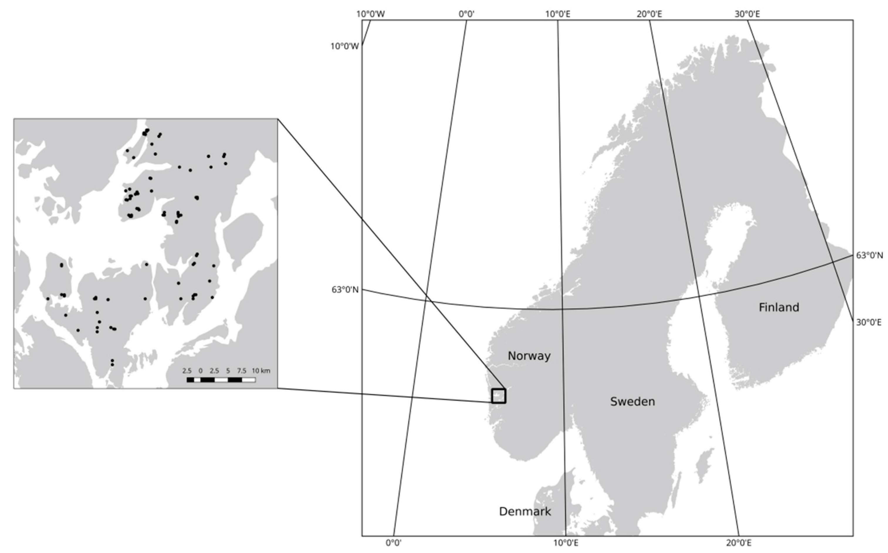
The study area is within the Fusa and Tysnes municipalities on the western coast of Norway (60°2′N, 5°46′E, 0–500 m above sea level, Figure 1). The forest is naturally dominated by Scots pine and deciduous species, mainly birch (Betula pubescens). From the 1940s and throughout the second part of the twentieth century, regeneration using non-native tree species—such as Sitka spruce—was common in this region on the west coast of Norway. Note that Norway spruce is also considered non-native in parts of this region. The productive forest area is about 260 km², and the species composition is approximately 13% spruce, 66% pine, and 20% deciduous trees.

2.2. Field Data

Three sets of field observations were utilized in the present study, with observations from a total of 240 individual locations. All locations were situated in a spruce-dominated forest, and the proportions of Sitka spruce and Norway spruce were recorded for all locations. A total of 113 locations were dominated by Sitka spruce, and 127 were dominated by Norway spruce. Two of the sets were initially collected as a part of the data acquisition in other research and forest inventory projects. The three datasets are described in the following sections.

2.2.1. Forest Inventory Plots

A set of sample plots with the main purpose of being used to create forest management plans were utilized in the present project. These circular sample plots were measured during the summer of 2012 and had a size of 250 m². The sample plots were clustered, with up to nine plots in each cluster. The spacing between sample plots in the cluster was 250 m, and there was 3 km between clusters in the north and east directions. In the clusters, 1–5 plots were measured. Within the plots, all trees with a diameter at breast height >4 cm were calipered, and the height measured, on selected sample trees. Species-specific allometric models were then used to derive stem volume. The aggregated volume at each plot was used to determine species proportions. A species with a proportion of more than 50% was considered to be dominant.

From this initial set of plots, a sub-sample of 57 plots dominated by either Norway spruce or Sitka spruce were used in the present study.

2.2.2. Research Plots

A second set of field observations was from sample plots measured during the autumn of 2013. These circular sample plots had a size of 250 m² and were laid out in clusters of three in a triangular design. The internal distances between plots within the clusters were 20 m. A total of 93 plots dominated by Norway spruce or Sitka spruce were used from this set in the present study. Tree species proportions were derived following the same procedure as that of the forest inventory plots described above.

2.2.3. Additional Sitka Spruce Field Locations

Field measurements with the main purpose of increasing the number of observations from locations dominated by Sitka spruce was carried out during the summer of 2015. From an initial set of all forest stands in the study area dominated by Sitka spruce, 30 stands were subjectively chosen for measurements. With an initial goal of having the observations evenly spread out in the study area, the selection was ultimately guided by accessibility from, e.g., forest roads. The selection of the 30 stands were carried out prior to visiting the stands in the field, with the exception of a few occasions in which a nearby stand was measured instead due to severe storm felling in the originally chosen stand. Within the selected stands, three locations were subjectively chosen, guided by these criteria: the locations are evenly spread out in the stand and are preferably not close to stand borders. At each of the three locations, the proportions of the basal area of Sitka spruce versus other species were recorded using a relascope.

2.2.4. Plot Positioning

For the first two datasets, the plot centers were positioned using survey-grade global positioning system (GPS) equipment. The forest inventory plots were positioned using real-time kinematic GPS, and the research plots using differential GPS with post-processing. In the post-processing, the three closest base-stations operated by the Norwegian mapping authority were used. A hand-held GPS receiver was used to record the position for the additional Sitka spruce plots.

2.3. Remote Sensing Data

We tested and compared three sources of remote sensing data in the present study, namely, Landsat 8 satellite imagery, orthophotos created from aerial imagery, and data from ALS.

2.3.1. Landsat 8

A search restricted to images in the period from 11 February 2013 to 31 August 2015 with less than 30% cloud coverage returned 30 potential images covering the study area. Of these, seven were selected for further use based on manual inspection for the distribution of clouds. The Landsat images had a pixel size of 30 m, and the acquisition dates for the seven Landsat images were:

• #1: 10 July 2013,
• #2: 26 July 2013,
• #3: 15 September 2014,
• #4: 6 November 2013,
• #5: 30 March 2014,
• #6: 15 April 2014, and
• #7: 1 May 2014.

The raw digital numbers were converted to top-of-atmosphere reflectance with correction for solar angle. This conversion was carried out using the rescaling coefficients provided in the Landsat 8 product metadata. The scene center solar angle was used for the solar angle correction. The approach is similar to the one used by Baig et al. [15].

2.3.2. Aerial Imagery—Orthophoto

Norway has a system for acquiring aerial images on a routine basis. The orthophotos produced from these images are made readily available on the Internet for end-users. The orthophotos used in the current study have a resolution of 0.25 m and were created from imagery acquired in July 2013.

2.3.3. Airborne Laser Scanner Data

ALS were acquired using an Optech ALTM Gemini instrument mounted on a PA31 Piper Navajo fixed-wing aircraft. The data acquisition was carried out from 5 June to 7 August 2010. The initial processing of the ALS data was carried out by the contractor according to standard procedures. Echo heights were normalized using a triangular irregular network (TIN) created from ground echoes identified using the progressive TIN densification algorithm [16,17].

2.4. Variable Extraction

For all the field reference locations, numerical features were extracted from the remote sensing data, and these features—or variables in a modeling context—are described for each of the three datasets in the following sections.

2.4.1. Landsat 8

Field reference data were among the Landsat 8 data coupled with the pixel from the satellite images, which contained the recorded field position. From this pixel, spectral values from the bands of the Landsat image were extracted. We also computed the normalized difference vegetation index (NDVI) and three indices derived with a tasseled cap transformation [18]. Coefficients for the tasseled cap transformation were taken from Baig et al. [15], where these indices are further described.

An overview of the variables extracted from the Landsat images are given in

Table 1. Variables derived from the Landsat satellite imagery. Corresponding bands.

Variable	Band(s)
Red	4
Green	3
Blue	2
Near infrared (NIR)	5
Short wavelength infrared 1 (SWIR1)	6
SWIR2	7
NDVI	4 and 5
Brightness	2–7 (tasseled cap transformation)
Greenness	2–7 (tasseled cap transformation)
Wetness	2–7 (tasseled cap transformation)

.

2.4.2. Aerial Imagery—Orthophoto

Pixels were extracted from 250-m² circular areas centered at the field locations, corresponding in size to the forest inventory plots. Note that this size was also used for the locations with relascope measurements. Variables were then derived from the distribution of spectral values across these extracted pixels. All variables were derived separately for the red, green, and blue band. The distributions of the spectral values were captured as percentiles of the value distribution (see

Table 2. Variables derived per plot from the orthophotos.

Variable	Description
P10_red, P20_red … P90_red	10th, 20th, … 90th percentiles of the distribution of the red, green, and blue spectral values, respectively.
P10_green, P20_green … P90_green
P10_blue, P20_blue … P90_blue
Textural variables
mean	The textural variables were calculated separately for the red, green, and blue band. The variables are further described in Haralick et al. [20].
variance
homogeneity
contrast
dissimilarity
entropy
second moment
correlation

). Texture is commonly used in different image analysis tasks, and we included textural variables derived using co-occurrence matrices [19]. The glcm package [20] in the statistical software R [21] was used to calculate the textural variables. Textural variables derived with co-occurrence matrices are calculated for each pixel, and the value depends on a predetermined window size, which provides the number of neighboring pixels for inclusion in the calculations. We calculated two distinct sets of textural variables: (1) a set with the values of the textural features from the single center pixel at each field reference location—in this case, the side of the window was equal to the diameter of the 250-m² field plot, which means that the pixels included in the calculations approximately corresponded to the pixels within the circular field plot—(2) another set of textural variables derived by averaging the values for all pixels within the plot—in this latter case, the window size was reduced in order to limit the number of pixels outside the circular plot that was included in the calculations. The window side were, in this case, set to correspond to the radius of the 250-m² circular field plots (i.e. 8.92 m). Both these approaches caused some of the pixels outside the plot to be included in the calculation of textural variables.

An overview of the variables derived from the orthophotos is given in Table 2.

2.4.3. ALS Data

Laser echoes were extracted from 250-m² circular areas centered at the field locations. Within these circular areas, above-ground heights of the laser echoes were extracted, and percentiles and order statistics were obtained from the height distribution. These types of height-derived variables have been used in the estimation for forest inventories and have been shown to be well correlated with, e.g., timber volume [22]. To use these height metrics for classification, they were normalized to the maximum echo height (See

Table 3. Variables derived from the airborne laser scanner (ALS) data.

Variable	Description
Hmean	Mean echo height relative to the maximum echo height.
Hsd	Standard deviation of the echo height distribution.
Hcv	Coefficient of variance for the echo height distribution, relative to the maximum echo height.
Hkurt	Kurtosis of the echo height distribution.
Hskewness	Skewness of the echo height distribution.
H10, H20 … H90	The 10th, 20th, … 90th percentile of the height distribution of the laser echoes, relative to the maximum echo height.
d0, d1, …. d10	Density variables. Number of echoes above equally spaced height intervals.
imax	Maximum echo intensity.
imean	Mean echo intensity.
isd	Standard deviation of the echo intensity distribution.
icv	Coefficient of variance for the echo intensity distribution.
ikurt	Kurtosis of the echo intensity distribution.
iskewness	Skewness of the echo intensity distribution.
i10, i20 … i90	The 10th, 20th, … 90th percentile of the intensity distribution of the laser echoes.
i0, i1, …. i10	Number of echoes above equally spaced height intervals in the echo intensity distribution.

). In addition to an accurate position, each recorded laser echo is also associated with an intensity value, giving the intensity of the reflected laser light. Previous studies show that these intensity values might hold information that can be used to discriminate between different tree species [5,23]. We therefore included variables describing the distribution of intensity values, which corresponded to the variables derived from the height distribution.

A summary of the variables derived from the ALS data is given in Table 3.

2.5. Classification Procedure and Algorithms

A binary classification was carried out with three types of classification algorithms: random forest, support vector machine (SVM), and logistic regression.

The classification was carried out using a leave-three-out cross-validation procedure. Three observations were held back as validation data, and the remaining 237 observations were used to build the classification. The observations were grouped according to the clusters in the field data, which ensured that all observations from the same cluster or stand were in the same group, and thus did not occur in the calibration and validation set at the same time. The procedure was repeated 80 times until all groups of three observations had been used for validation once. The predictions for each validation iteration were recorded, and accuracy statistics computed.

Models were fit with the variables derived from the remote sensing datasets, given in Table 1, Table 2 and Table 3, with modeling and cross-validation carried out for each combination of a remote sensing dataset and a classification algorithm. Models were also fit to combinations of two out of three sets of remote sensing data.

Spectral differences between species can vary throughout the year, and we used data from individual Landsat images from different points in time, as well as a combination of data from multiple Landsat images.

2.5.1. Random Forest and SVM

Random forest is a machine-learning classification algorithm and is based on multiple binary classification trees, grown with bootstrap samples of data. It was introduced by Breiman [24] and is used for classification and regression. SVM is another widely used machine-learning classification algorithm based on constructing optimal separating hyperplanes in transformed versions of data. Classification with random forest, SVM, and logistic regression is further described by Hastie et al. [25].

The classification with the random forest algorithm was carried out using the randomForest package in R [26]. Default values for adjustable parameters were used. Classification with SVM was carried out using the svm function from the e1071 package in R [27]. Default values for adjustable parameters were also used for the SVM models.

2.5.2. Logistic Regression

The logistic regression models were fit with the glm function in R, using the step function to do a stepwise variable selection. The variable selection was applied in order to avoid correlated variables, i.e. multicollinearity. The stepwise procedure was carried out using the Bayesian information criterion (BIC) for selection. Both forward and backward selection was enabled with an empty model as the initial model. Finally, the glmulti function in the glmulti package [28] in R was used to select the best model from all possible subsets of the variables selected through the stepwise selection procedure. In this final model selection, BIC was used as a criterion, and only models with less than six variables were considered.

The predicted classes were derived from the logistic regression by using a cut-off value of 0.5, i.e. observations with a modeled probability of > 0.5 were classified as being dominated by Sitka spruce.

2.6. Accuracy Assessment

The classification performance for each model was assessed by computing the overall, user, and producer accuracy for the Sitka class, as well as the kappa statistic.

The user accuracy corresponds, in this case, to the probability that a location classified as being dominated by Sitka spruce really belong to this class. Conversely, the producer accuracy is the probability that a location dominated by Sitka spruce is in fact classified as such.

The kappa statistic—also referred to as Cohen’s kappa—is a measure of the overall accuracy, and is well suited for comparison of different models solving the same classification problem. There are several ways of interpreting the kappa value; Landis and Koch [29] considers 0–0.20 as slight, 0.21–0.40 as fair, 0.41–0.60 as moderate, and 0.61–0.80 as substantial.

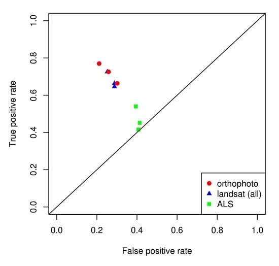
The results were also plotted in a “receiver operating characteristic” (ROC) space [30], enabling a visual comparison of the different data sources and classification algorithms.

3. Results

The overall results from the cross-validation procedure show a slight to moderate ability to discriminate between observations dominated by Norway spruce and Sitka spruce, using the remote sensing data. The resulting kappa values varied between 0.075 and 0.576 for the tested combinations of remote sensing data and classification methods (

Table 4. Accuracy statistics from the cross-validation of the classification models. User and producer accuracy for the Sitka class. The table is sorted according to the kappa value, i.e. the models with best performance appear at the top of the table. The use of data from individual or a combination of all seven Landsat images are indicated by image number (see Section 2.3.1 for dates of individual images). The dots indicate the combination of classification algorithm and datasets used.

Overall Accuracy	Kappa	User Accuracy	Producer Accuracy	Logistic Regression	SVM	Random Forest	Orthophoto	Landsat	ALS
0.788	0.576	0.746	0.832	•				#1
0.783	0.566	0.765	0.779	•				#1	•
0.767	0.533	0.744	0.770	•			•
0.750	0.496	0.752	0.699	•			•	#1
0.746	0.491	0.724	0.743		•		•	#1
0.738	0.471	0.736	0.690	•			•		•
0.733	0.462	0.738	0.673	•				#3
0.729	0.456	0.714	0.708			•	•		•
0.725	0.449	0.701	0.726	•				all
0.717	0.428	0.723	0.646			•		all
0.713	0.425	0.683	0.726		•		•
0.708	0.414	0.694	0.681		•		•		•
0.704	0.405	0.694	0.664		•			all
0.704	0.405	0.694	0.664			•	•	#1
0.696	0.387	0.689	0.646			•		#2
0.696	0.387	0.689	0.646			•		#3
0.679	0.356	0.658	0.664			•	•
0.675	0.344	0.673	0.602	•				#2
0.663	0.320	0.651	0.611		•			#2
0.667	0.316	0.739	0.451	•				#7
0.654	0.304	0.642	0.602			•		#6
0.650	0.293	0.644	0.575			•		#1
0.642	0.287	0.603	0.699		•			#5
0.638	0.272	0.616	0.611		•			#3
0.633	0.264	0.611	0.611			•		#7
0.638	0.259	0.671	0.451					#1	•
0.629	0.255	0.607	0.602		•			#7
0.629	0.254	0.611	0.584	•				#6
0.625	0.252	0.592	0.655			•		#5
0.625	0.243	0.614	0.549			•		#1	•
0.617	0.228	0.600	0.558		•			#4
0.608	0.221	0.573	0.664	•				#5
0.613	0.216	0.604	0.513		•			#6
0.617	0.213	0.657	0.389		•			#1
0.596	0.175	0.603	0.416		•				•
0.588	0.170	0.565	0.540	•					•
0.579	0.146	0.567	0.451			•			•
0.550	0.099	0.521	0.540			•		#4
0.529	0.075	0.500	0.690	•				#4

). When plotting the results in a ROC space, it is evident that there is a spread in the results, both in terms of classification algorithms and data sources (Figure 2).

We conducted classification with data from each of the single Landsat images, as well as a combined dataset with data from all seven images. Each of these eight sets of data was further combined with data derived from ALS and orthophotos. Finally, these different sets of data were used in combination with three classification algorithms: logistic regression, SVM, and random forest. The combinations of data and algorithms are given in Table 4. The best results was in the present study obtained by using data from Landsat image #1, with a kappa value of 0.576 and a corresponding overall classification accuracy of 79% (Table 4). When comparing the classification results with each of the three types of remote sensing data, it is clear that the use of ALS data alone produced poor results, whereas the data from spaceborne or airborne images performed better (Figure 2b). In the case of combining data from the best Landsat image with data from airborne sensors, there were no improvements over the use of Landsat data alone (Figure 2d and Table 4).

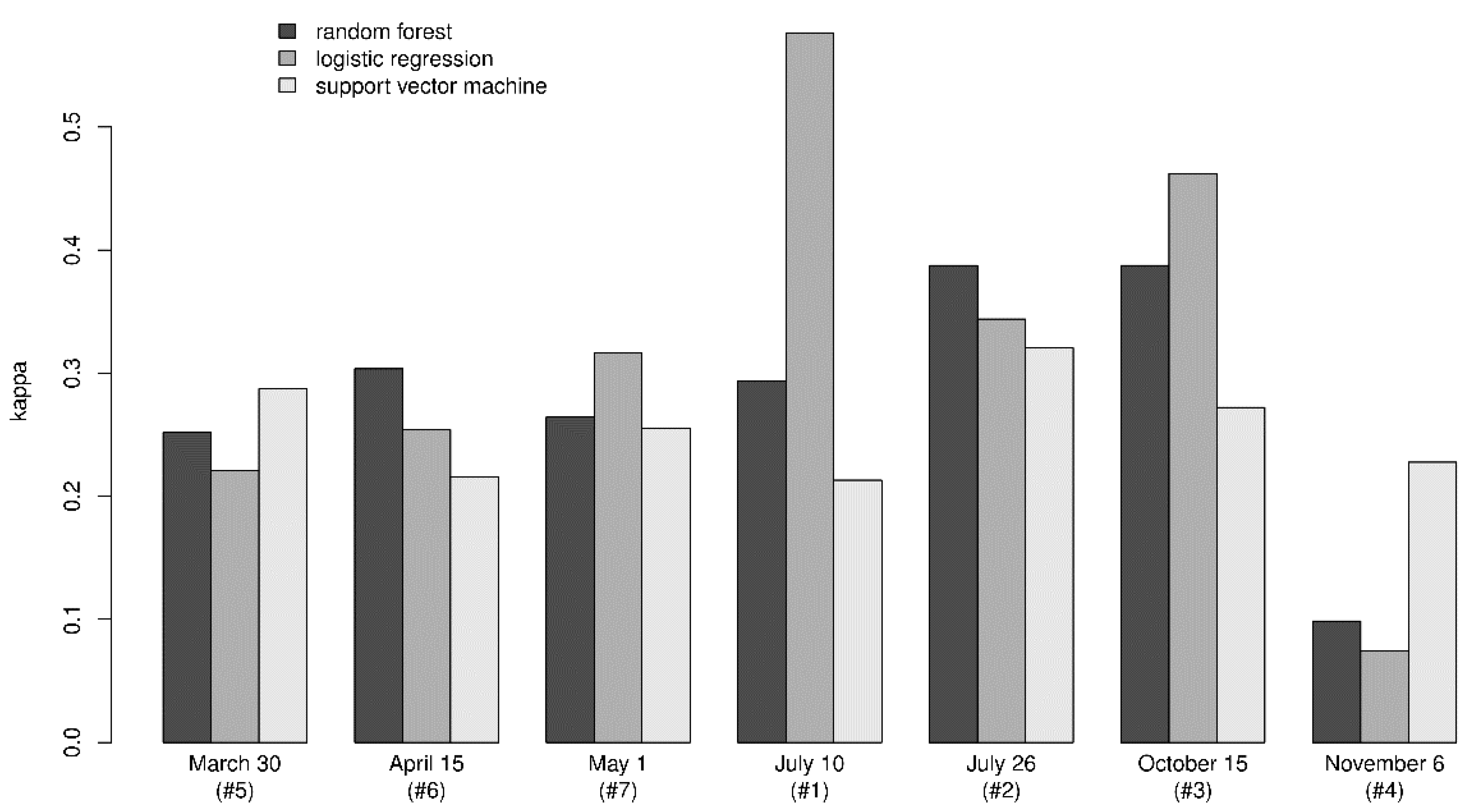
When inspecting the results from the classification using data derived from single Landsat images alone, it is evident that the accuracies vary, with kappa values ranging from 0.228 to 0.576 (Table 4, Figure 2c and Figure 3). Models with data from Landsat image #1 and #3 performed best, with kappa values of 0.576 and 0.462, respectively. When inspecting the results with respect to acquisition dates, there seems to be higher classification accuracies in the present study when using Landsat images acquired in the summer (Figure 3). Comparing the results obtained with the three classification algorithms, there seems to be slightly better results when using logistic regression (Figure 2a and Figure 3).

4. Discussion

There are few directly comparable studies, but the accuracy obtained in the present project seems to be within the range of accuracies obtained in some related studies. Carter et al. [6] used imagery from Landsat 5 to classify an invasive tree species in Colorado (US) and obtained an overall accuracy of 80%. Higher accuracies than in the present study were obtained in some studies using satellite imagery with a higher resolution, such as Fuller [7]. The classification accuracies in that study are also higher than the accuracies obtained with high-resolution orthophotos and ALS in the present project. One reason could be that the spectral and structural differences between Sitka spruce and Norway spruce are too small, or of such a nature that they are not well captured in the remote sensing data. Vauhkonen et al. [12] notes that the task of inter-genera separation of species is challenging, and in species classification using remote sensing the species are typically from different genera.

In the present study, the best model used data derived from Landsat image #1, with a kappa value of 0.576 when using only Landsat data. The best model using data from Landsat image #4 on the other hand, had a kappa value of 0.228. This indicates that the inherent information that reveal differences between Norway spruce and Sitka spruce is not present to the same degree in all seven Landsat images. Using a single Landsat image for this kind of classification is, in other words, sensitive to the selection of the image, and it could therefore be a solution to test multiple images or to use multitemporal data. The results could suggest that satellite imagery acquired in the summer yields a better classification, indicating that the differences between the two species are greater in the growing season. Spruce trees have light-colored shots, which darken during the summer. Slight differences in the onset of growth or the darkening of the new shots might enhance the spectral differences between the two species. This could be one explanation for the better classification results when using data from Landsat images acquired during the summer. Another influencing factor could be the fact that the elevation angle of the sun is potentially larger in the summer at this latitude. This means that the images will be less affected by shadows, which might lead to a clearer distinction between the two species. Effects of shadows due to topographic features can, however, be mitigated by correcting the images using a topographic normalization. Finding optimal points in time for discriminating between Norway spruce and Sitka spruce using Landsat images could be subject to further research.

Compared to the models based on data from the two airborne sensors, the satellite imagery performed well in this comparison despite a lower spatial resolution. Using data with a lower spatial resolution does, however, restrict the possible spatial levels for predictions.

Combination of data from different sources did not yield predictions with considerable higher accuracies in this comparison. Adding data from ALS or orthophotos did, however, slightly increase the classification accuracy when compared to the use of Landsat imagery alone.

Three types of classification methods were tested in the present project, with logistic regression yielding the best results. The logistic regression was, however, implemented with a variable selection procedure which was not used for the other two approaches. Any conclusions drawn from the performance of the different models should incorporate this, and future research could reveal if the two machine-learning procedures would benefit from the use of a variable selection procedure with this type of data. Dalponte et al. [31] did, however, find little effect of variable selection in a related classification task.

The field measurements were carried out on circular plots of 250 m² in the current study, which means that the field measurements do not directly correspond with the 30 × 30 m pixels from the Landsat imagery. For any given plot, the chosen Landsat pixel will therefore at least cover 650 m², which were not inventoried on the ground. If the field plot happens to lay on the border between pixels, an even greater part of the chosen pixel will cover areas outside the field-measured plot. In addition, we used one set of field observations positioned with a hand-held GPS receiver. The expected accuracy of this positioning might lead to errors in the spatial alignment between these field observations and the remote sensing data. With respect to these two related issues, we would like to note that all field observations of dominant species were carried out within relatively homogeneous stands. It is therefore reasonable to assume that the dominant species observed within the 250-m² plot is similar to the species dominating the whole stand, i.e. the area surrounding the field plot. Spatial misalignment will in that case have less effect on the results. Neighboring stands with different species proportions could nevertheless still introduce errors if they are within the area from which the remote sensing data are taken. Others, however, have used similar combinations of field and remote sensing data [32,33].

Field and remote sensing data were in the present study acquired over a period of five years. Time differences between sets of data can introduce errors, since conditions on the ground might change between the acquisition of field reference and remote sensing data. In the present study, we registered dominant tree species in a mature forest, which, in Norway, is a property that is highly unlikely to change within a timespan of five years. We do therefore assert that the effect of the time differences, in this case, is small.

Since the remote sensing data in the present study were obtained from above, crown coverage will provide the best representation of the species proportions, as these are contained in the remote sensing data. Nevertheless, species composition is often derived by available field measured attributes such as volume, basal area, and number of stems—not by crown coverage, which is very difficult to measure in field.

In an operational setting, the identification of spruce-dominated areas must be carried out prior to the classification described in the current study. There are several possible approaches to this task, one could be to first classify spruce as one of several tree species classes. This spruce-class could then be subsequently classified into Norway spruce and Sitka spruce. Classification of forested and non-forested areas could be done using ALS data if available, since the above-ground vegetation structure is precisely the type of information that is contained in the data from these sensors. The overall obtainable classification accuracy when classifying Norway spruce and Sitka spruce in such an operational approach could be subject to further research.

5. Conclusions

Overall, the results in the present study show a slight to moderate ability to discriminate between stands dominated by Norway spruce or Sitka spruce using Landsat 8 imagery. The overall classification accuracy obtained for classification with data from single Landsat images varied between 53% and 79%, and the results indicate that there are systematic differences between images acquired at different times of the year. This could be subject to further research. The use of combined data from multiple Landsat images did not improve the classification accuracy here. Nor did using additional data from airborne sensors yield considerable higher classification accuracies. The accuracy when classifying Norway spruce and Sitka spruce in an operational setting will also rely on the ability to discriminate between spruce-dominated forests and other vegetation and land cover types.