Development, Production and Evaluation of Aerosol Climate Data Records from European Satellite Observations (Aerosol_cci)

Abstract

Producing a global and comprehensive description of atmospheric aerosols requires integration of ground-based, airborne, satellite and model datasets. Due to its complexity, aerosol monitoring requires the use of several data records with complementary information content. This paper describes the lessons learned while developing and qualifying algorithms to generate aerosol Climate Data Records (CDR) within the European Space Agency (ESA) Aerosol_cci project. An iterative algorithm development and evaluation cycle involving core users is applied. It begins with the application-specific refinement of user requirements, leading to algorithm development, dataset processing and independent validation followed by user evaluation. This cycle is demonstrated for a CDR of total Aerosol Optical Depth (AOD) from two subsequent dual-view radiometers. Specific aspects of its applicability to other aerosol algorithms are illustrated with four complementary aerosol datasets. An important element in the development of aerosol CDRs is the inclusion of several algorithms evaluating the same data to benefit from various solutions to the ill-determined retrieval problem. The iterative approach has produced a 17-year AOD CDR, a 10-year stratospheric extinction profile CDR and a 35-year Absorbing Aerosol Index record. Further evolution cycles have been initiated for complementary datasets to provide insight into aerosol properties (i.e., dust aerosol, aerosol absorption).

1. Introduction

Aerosols influence the distribution of radiation, both directly by scattering, absorbing and emitting radiation and indirectly by acting as condensation or nucleation sites in clouds. The indirect effect influences the hydrological cycle through impacts on cloud properties, cloud lifetime, precipitation and atmospheric stability (as absorbing aerosols alter local heating rates in distinct layers). In the stratosphere, they play a crucial role in ozone chemistry and ozone depletion through their contribution to the formation of polar stratospheric clouds. IPCC (Intergovernmental Panel on Climate Change) assessments confirm that the aerosol indirect effect remains the largest uncertainty in understanding the evolving climate [1,2]. Beyond their climate relevance, atmospheric aerosols also play an important role in air quality and its consequences to human health.

Global observation is necessary to understand the role of atmospheric aerosols in the climate system and to monitor changes in their abundance and composition. Obtaining such observations with validated accuracy and precision is not straightforward. Satellite instruments are capable of providing global observations of the last few decades (see, e.g., [3,4,5]). To be used properly, their information content needs to be validated over a variety of regions. Global aerosol models can provide a comprehensive picture and fill gaps between satellite measurements (or even provide additional types of dataset). However, such results depend on a model’s ability to describe all relevant processes and its underlying initialization data (e.g., emissions). Therefore, model data also require validation. Ground-based and airborne observations provide limited spatial and temporal coverage but use instruments specifically designed to measure aerosol properties. Furthermore, they allow accurate observation of local features. Additionally, ground-based instruments typically have better accuracy than satellite remote sensing and are, therefore, often used as validation datasets. The comparison between satellite, model and ground-based observations ultimately reveals the strengths and limitations of each observing system. By properly integrating them, understanding and monitoring of the Earth system at all relevant scales can be facilitated. In light of the next round of experiments by the Coupled Model Inter-comparison Project (CMIP-6) to prepare for the next IPCC assessment, there is a need for well-qualified, satellite-based, aerosol Climate Data Records (CDRs).

Aerosols are highly variable in their composition and spatial concentration, as a result of many natural and anthropogenic sources and processes. This complexity requires observing several variables to understand and monitor the role of aerosols in the climate system. This cannot (yet) be done by exploiting one single sensor but requires the combination of different instruments with complementary information content. The Global Climate Observing System (GCOS) sets out observation requirements from satellites for aerosols as one ECV (Essential Climate Variable) [2]: The variables needed are aerosol optical depth (AOD), single scattering albedo (SSA), vertical extinction profiles and layer height.

The user requirements of GCOS [2] provide a generalized statement of the required data record characteristics. For AOD at 550 nm, it states the need for an accuracy better than 10% or 0.03 (whichever is larger), with a horizontal resolution of 5–10 km, a temporal resolution of 4 h and a stability of 0.01 per decade. Single scattering albedo requires an accuracy of 0.03 and stability of 0.01 per decade at the same spatio-temporal resolution as AOD. Aerosol extinction profiles require a horizontal resolution of 200–500 km, a vertical resolution lower than 1 km near the tropopause and of about 2 km in the middle stratosphere, and a temporal resolution of one week. Accuracy and stability should be of 10% and 20% respectively. In general, user requirements differ substantially for different applications (e.g., monitoring, trend analysis, model development/initialization, process studies), which is not considered in detail in the CGOS satellite supplement [2], but is taken into account in the collection (so-called “rolling review”) of requirements by WMO (World Meteorological Organization).

GCOS has also published a set of principles for producing satellite climate data records [6]. These principles cover the design of space and ground hardware to ensure uninterrupted observations of sufficient quality and stability to meet user needs for climate research. The principles discuss documentation (algorithms, metadata), testing, and regular assessments of the algorithms used to produce climate data records. Operational capability for data access and user support is requested. Further demands cover the specification of users’ needs as a basis for instrument design, the evaluation of homogeneity and consistency, and sustained production. Complementary in situ data need to be available as reference and uncertainties in the satellite products have to be quantified.

A CDR is nominally required to contain a time series of 30 or more years. As individual satellite missions have shorter lifetimes (e.g., designed for 5 years, but may last 15), a CDR must be built from multiple data records. Even though operational systems assure continuity by launching a series of identical sensors, their characteristics may change due to large mechanical stresses during launch and post-launch optical degradation or orbital drift. If similar, but not identical, instruments are used then the impact of the differences needs to be assessed in the derived aerosol products. For example, [7] studied a three-year overlap characterizing the AOD time series of the NASA (National Aeronautics and Space Administration) MODIS (Moderate Resolution Imaging Spectro-Radiometer) and NOAA (National Oceanic and Atmospheric Administration) VIIRS (Visible Infrared Imaging Radiometer Suite) instruments when applying both identical and distinct algorithms.

The longest available satellite aerosol CDRs include AOD over ocean AVHRR (Advanced Very High Resolution Radiometer)—time series back to early 1980s; [8,9]) and Absorbing Aerosol Index from several spectrometers TOMS (Total Ozone Mapping Spectrometer)—time series back to 1978; [10,11], and the data record described in this paper). A quantitative absorption record (single scattering albedo) with OMI (Ozone Monitoring Instrument) starts in 2005 [12]. The earliest suitable AOD data records over land extend back into the mid-1990s ATSR-2 (Along Track Scanning Radiometer No. 2) from 1995 as described in this paper and SeaWIFs (Sea-viewing Wide Field-of-view Sensor) from 1997 to 2010; [13]). For stratospheric aerosols, time series of extinction at 1 µm were developed from satellite measurements back to 1978 [5,14]. More than 16 years of stratospheric particle size distribution parameters have been developed from the SAGE II (Stratospheric Aerosol and Gas Experiment) experiment [15,16,17].

In the European Space Agency (ESA) Climate Change Initiative (CCI; [18]) the Aerosol_cci project has worked on the development and qualification of several complementary aerosol CDRs. The major goal of this activity, which started in 2010, has been to produce aerosol CDRs which satisfy the requirements on data quality and transparent documentation set by GCOS. As first steps towards this goal, several algorithm experiments [19] and a round robin exercise [20] for total AOD were performed. Algorithms for stratospheric aerosol extinction and an absorbing aerosol index were also evaluated. Based on these early analyses, a full re-processing of complete mission time series has started within an iterative evolution cycle. Work on additional variables, such as dust AOD and aerosol typing, was added to increase the information content.

With this paper we want to share the scientific and programmatic experiences during climate-quality aerosol data records production. We demonstrate the iterative development and evaluation cycle with an AOD CDR from dual-view radiometers in Section 2. Section 3 describes additional specific elements of AOD data record evaluation. The applicability of the iterative approach to other aerosol datasets is then illustrated in Section 4 with four complementary aerosol datasets. Section 5 summarizes and discusses lessons learned and conclusions.

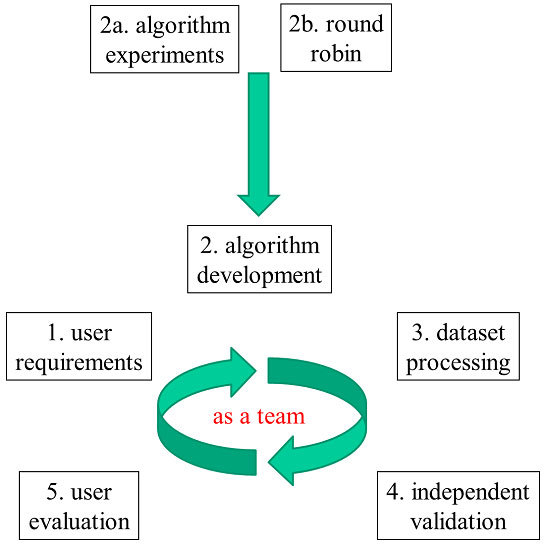
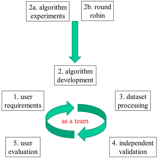
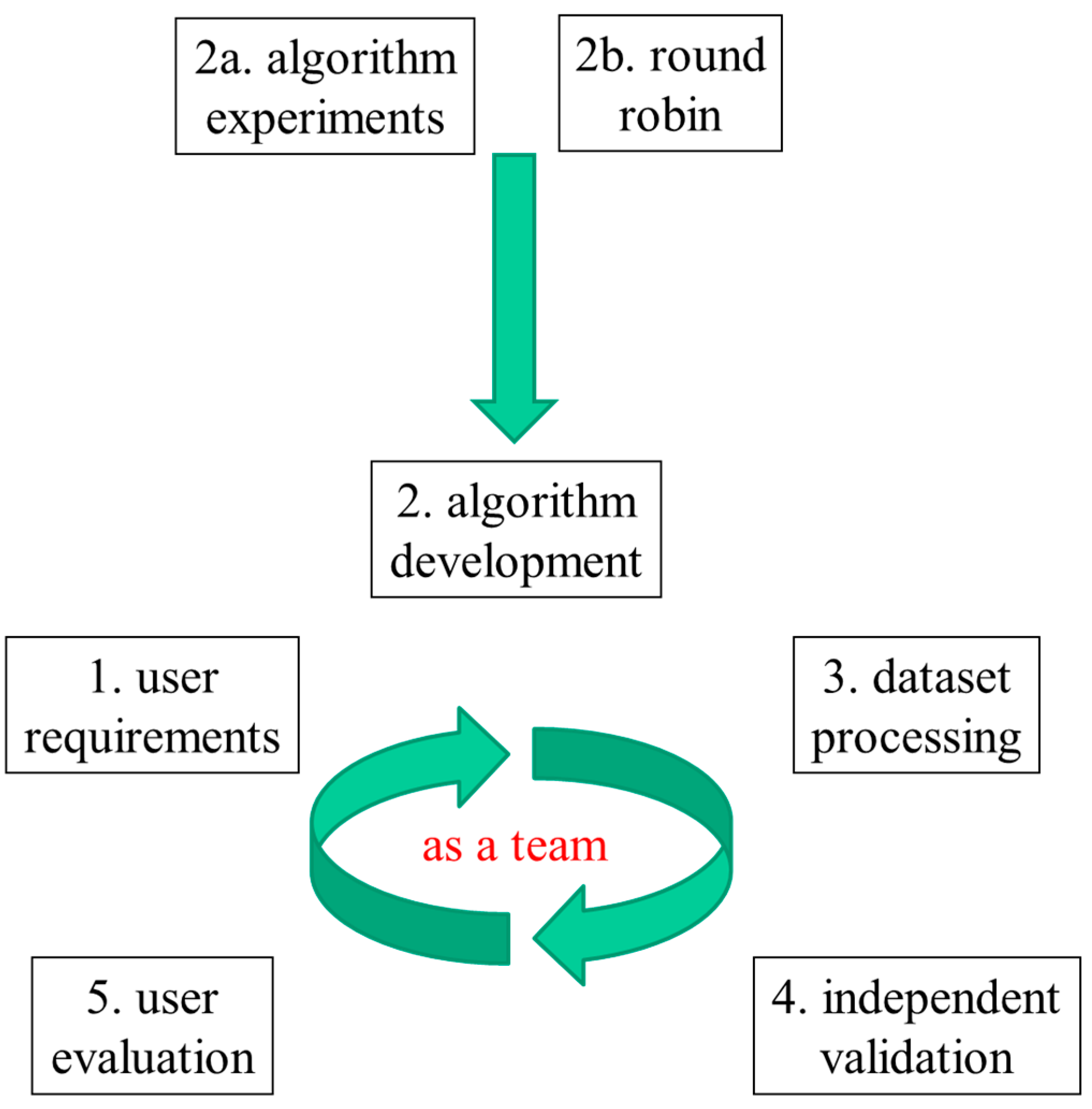
2. Iterative Algorithm Development and Evolution Demonstrated with ATSR AOD CDRs

2.1. General Approach

In order to satisfy the GCOS climate monitoring principles [6] and provide aerosol CDRs of the best possible quality, a cyclic approach has been implemented (see Figure 1). Iteration of this sequence of steps has proven necessary, since aerosol retrieval algorithms have to make use of experimental elements due to the ill-posed nature of the underlying retrieval problem (e.g., use of auxiliary/climatological datasets, simplifications of aerosol models and surface treatment). It can thus not be expected that theoretical considerations alone will solve all problems. The successful use of such experimental elements is based on a retrieval expert’s experience and can only be justified through validation of the resulting dataset.

The cycle starts with the application-specific refinement of user requirements (building on GCOS requirements, [2]). In our case, requirements from specific user communities are added. Algorithm development is then conducted and small quantities of data are processed and undergo independent validation (comparison to reference datasets which have a smaller error than the satellite data products). Finally, the time series are tested by users in concrete applications to understand their value, strengths and limitations in various domains. The loop closes by comparing the original requirements to the data assessment and identifying remaining needs for improvements. In each iteration more demanding requirements to tackle new scientific questions and applications may need to be included. During all steps, users, algorithm developers, validation experts and system engineers remain in close dialogue. A similar concept has been presented in the context of satellite data uncertainty characterization by [21].

Algorithm development can start with preparatory elements: Algorithm experiments identify key sensitivities or areas for harmonization across a set of algorithms (e.g., [19]). As one example, a common definition of optical aerosol components was defined and implemented within eight different AOD algorithms. Other modules, such as cloud masking or surface treatment, were shown to be algorithm-intrinsic (and were therefore not harmonized). To avoid cloud contamination, post-processing was found to be most efficient excluding AOD outliers which are probably cloud contaminated [22].

A round robin exercise (e.g., [20]) conducts a validation of several precursor algorithms against external references, comparing their results. A precursor algorithm has already reached a minimum standard of maturity and documentation (nominally a peer-reviewed publication of its principles). This round robin exercise allows the selection of algorithms with suitable quality for large-scale processing and further developments.

The amount of data processed and validated may increase during the evolution of both the algorithms and their processing systems. Assessments may start with small data amounts, sufficient to understand sensitivities during algorithm experiments (e.g., one month of global data), extend to more comprehensive volumes (e.g., covering all seasons) and finally consider full-mission time series.

2.2. New ECV CDRs from Two Dual-View ATSR Radiometers

This section outlines an implementation of the development and evaluation cycle of Figure 1. Total AOD is retrieved using three different algorithms, each based on different principles, applied to the ATSR instruments (ATSR-2 onboard ERS-2 (European Remote Sensing Satellite 2), useful for aerosol retrieval from 1995 until 2003; and AATSR (Advanced Along-Track Scanning Radiometer) onboard ENVISAT (ESA’s Environmental Satellite), used from March 2002 until April 2012). The datasets from these two instruments have an overlap of about one year. Three algorithms, ADV/ASV (AATSR Dual/Single View), in brief denoted as ADV), ORAC (Oxford RAL Aerosol and Cloud retrieval) and SU (Swansea University), are used. An overview of the ATSR-2/AATSR datasets discussed in this paper is presented in

Table 1. Overview of ATSR (Along Track Scanning Radiometer) data records and algorithms discussed in this paper.

Vertical	Parameter	Sensor(s)	Coverage, Resolution	Algorithm, Version	Characteristics	References
Total column	AOD 0.55 µm, 0.67 µm, 0.87 µm	ATSR-2 AATSR	1995–2003 2002–2012 global 10 × 10 km, 6-daily 1° × 1° daily/monthly	Principle: dual view radiometer in the visible and near-infrared; thermal infrared for cloud masking
				ADV/ASV V2.30	LUT approach	[20]
					land surface: spectral constant reflectance ratio	[23]
					ocean surface: modelled reflectance	[24]
					aerosol model: mixing Aerosol_cci common components	[20]
					cloud mask: combined thresholds,	[25]
					post-processing	[26]
				ORAC V3.02	optimal estimation	[27]
					land surface: bi-directional reflectance model	[28]
					ocean surface: modelled reflectance	[29]
					aerosol model: mixing Aerosol_cci common components	[20]
					cloud mask: combined thresholds
				SU V4.21	Iterative model inversion	[30]
					land surface: bi-directional reflectance model	[28]
					ocean surface: modelled reflectance	[31]
					aerosol model: mixing Aerosol_cci common components	[20]
					cloud mask: combined thresholds	[26]

; for more extensive descriptions we refer to [20] or the references provided in Table 1.

These data records are freely disseminated through the Aerosol_cci ftp site ([32]; common account and password can be obtained from [33]). Datasets are provided in sensor projection (termed “level 2” or in short “L2” datasets) and as gridded datasets (named “level 3” or “L3”; aggregated into daily, weekly or monthly products).

Initially, the three ATSR algorithms were studied alongside five other AOD algorithms to identify modules for improvement [19]. A round robin exercise [20] selected these three algorithms as the most promising for future development. This benchmarking also found that no single algorithm demonstrated superior performance in all conditions.

2.3. Extended User Requirements from the Aerosol Climate Modelling Community

For an application-specific adaptation of the GCOS requirements, we focus on the climate modelling community (Aerosol Comparisons between Observations and Models AEROCOM, Aerosol-Cloud-Precipitation-Chemistry ACPC) supporting climate studies for IPCC (within CMIP). This community typically works with gridded model datasets (e.g., 1° latitude/longitude grid) to analyze long-term changes and trends in aerosols over regions of interest. Their representatives outline accuracy requirements that bridge the intrinsic satellite resolution and the grid model size. By averaging pixel-level AODs over space and time, the random part of their uncertainties can typically be reduced. Model analysis often studies large patterns, i.e., regional or seasonal homogeneous aggregations. To detect changes in those, accuracy requirements become more stringent with increasing spatial/temporal scale (

Table 2. Total column Aerosol Optical Depth (AOD) accuracy requirements as function of spatial/temporal resolution.

Total Column Properties
Property	Satellite Product	Model Grid	Regional	Inter-Annual	Decadal
Spatial Resolution	0.1° × 0.1°	1° × 1°	10° × 10°	10° × 10°	10° × 10°
Temporal Resolution	2 h	daily	monthly	seasonal	annual
AOD, 550 nm	0.04	0.02	0.01	0.008	0.006
Fine mode AOD, 550 nm	0.03	0.015	0.008	0.006	0.005
Absorbing AOD, 550 nm	0.01	0.005	0.003	0.0025	0.002
Dust AOD, 550 nm	0.03	0.015	0.008	0.006	0.005

). Furthermore, the rather weakly qualified GCOS need for “additional aerosol properties” is rationalized to mean parameters that are suitable for satellite retrieval and can be directly compared to model datasets. Fine mode AOD or dust AOD are highlighted as these can also serve as proxies for cloud condensation nuclei (CCN) or ice nuclei (IN), respectively, in aerosol-cloud interaction studies. Required accuracies for those quantities are derived by multiplying their maximum fraction of total AOD with the AOD accuracy.

2.4. Algorithm Development and Validation—Benefit of Repeated Development Cycles for ATSR Datasets

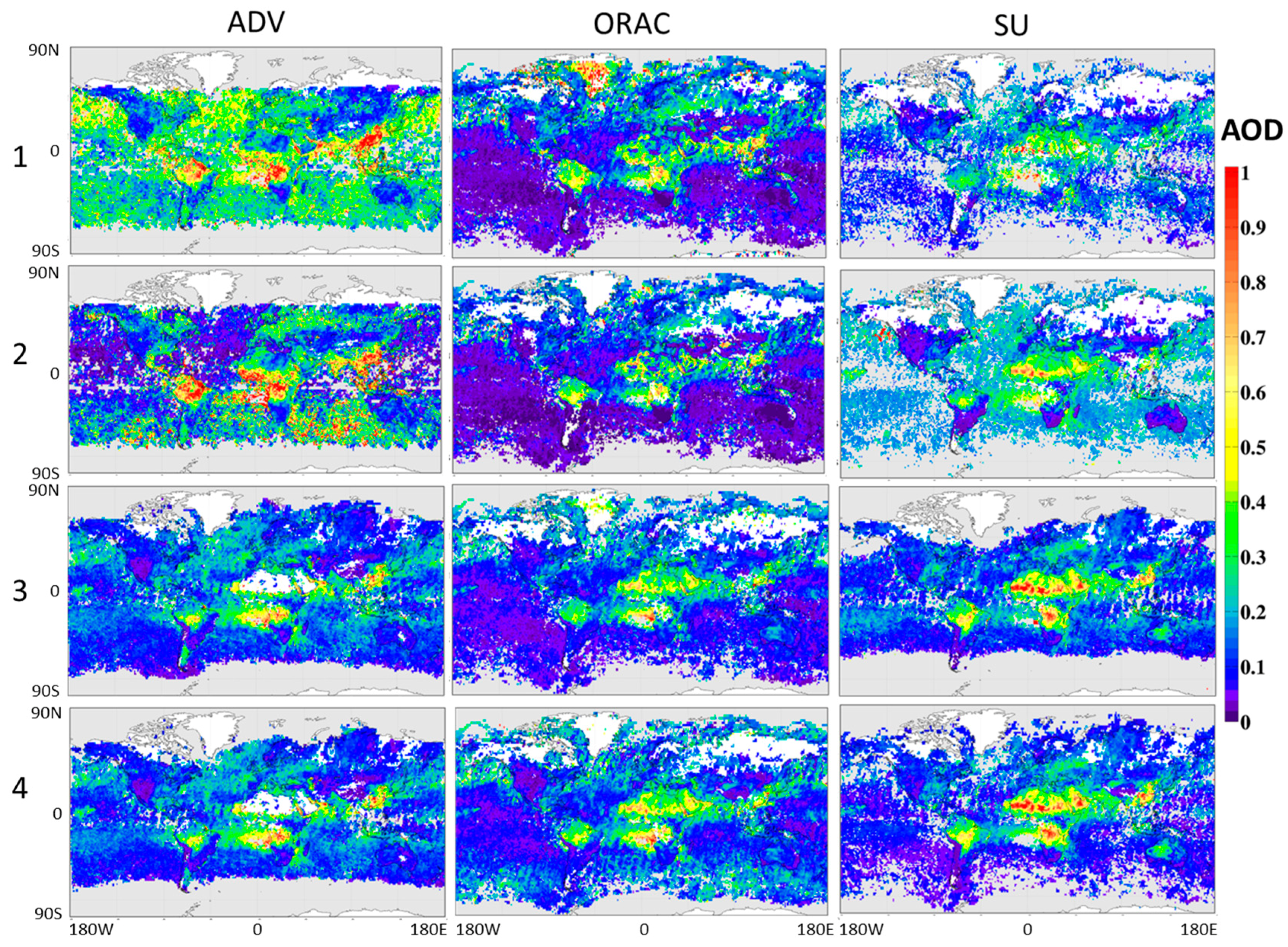
2.4.1. Overall Improvement of Algorithms

Iterative algorithm development and independent validation assure transparent and credible proof of any changes made. The cycle improves the individual algorithms while producing a convergence of their datasets. Our validation is based on comparison to independent data from the AERONET [34] and MAN [35] sun photometer networks [36]. The results are first validated for L2 products. A spatial threshold of +/−35 km and a time frame of +/−30 min is used to match satellite pixels with the independent data.

The following metrics are considered: Pearson correlation coefficients (K), bias, Root Mean Square Error (RMSE) of satellite retrieved AOD vs. the reference AOD data set and the fraction of retrieved pixels which satisfy the GCOS requirement for AOD accuracy (named “GCOS fraction”).

Table 3. Validation of the oldest and latest versions of the three AATSR (Advanced Along-Track Scanning Radiometer) AOD (aerosol optical depth) datasets vs. AERONET (Aerosol Robotic Network) AOD for September, 2008. Improved metrics are highlighted in green, metrics which became worse are in red colors.

Metric	Algorithm
	ADV/ASV		ORAC		SU
	V1.0	V2.3	V1.0	V3.02	V1.0	V4.21
Over Ocean
number of points	75	64	65	102	13	52
bias	0.04	0.02	0.07	0.10	0.06	−0.002
RMSE	0.16	0.09	0.15	0.16	0.08	0.06
correlation	0.58	0.89	0.81	0.93	0.89	0.86
GCOS fraction (%)	17	66	46	31	15	58
Over Land
number of points	306	185	262	262	138	343
bias	−0.005	−0.05	0.03	−0.002	−0.001	−0.01
RMSE	0.16	0.13	0.16	0.08	0.08	0.11
correlation	0.59	0.66	0.59	0.86	0.72	0.82
GCOS fraction (%)	37	54	40	51	46	62

shows these for the oldest and newest versions of the three AATSR algorithms (newest versions are 2.30 for ADV, 3.02 for ORAC and 4.21 for SU). This analysis evaluates only the small volume of data processed at the start of the development cycle (September 2008 global; [19]). All but three metrics improve after the development cycle. Similar results have been achieved for ATSR-2 despite smaller data volumes.

2.4.2. Algorithm Validation with Growing Data Volumes

A validation exercise should be designed such that its results are independent of the volume of data considered. Results drawn from excessively small comparison datasets can be misleading as the data may omit localized biases. However, it may not be appropriate to process full mission datasets in the early stages of algorithm evolution. To evaluate our procedure, we compare the validation results for AOD retrieved over land with the Swansea algorithm (v4.21) over three different data volumes: four months (one in each season) from 2008 (round robin exercise; [20]); the entire year of 2008; and the complete AATSR mission period 2002–2012 (Figure 2 and

Table 4. Validation of AATSR SU retrieved AOD (L2) v4.21 vs. AERONET AOD for different data volumes: one month of 2008, for four months of 2008, the whole year 2008, for years 2002–2012.

Metric	Data Volumes
	September 2008	March, June, September, December 2008	All 2008	2002–2012
Over Ocean
number of points	52	235	716	5808
bias	−0.002	−0.002	−0.002	0.006
RMSE	0.06	0.07	0.07	0.08
correlation	0.86	0.93	0.91	0.87
GCOS fraction	58	64	66	62
Over Land
number of points	343	993	3313	28,123
bias	−0.01	0.007	0.007	0.003
RMSE	0.11	0.12	0.14	0.15
correlation	0.82	0.86	0.81	0.79
GCOS fraction	62	56	51	52

). The top row shows scatter plots while the bottom row shows probability density functions (PDFs) of the difference between AOD values retrieved from satellite and AERONET (Aerosol Robotic Network). Those PDFs are separated for low and high aerosol loading (blue color corresponds to PDF for AOD > 0.2, red color corresponds to PDF for AOD < 0.2, black color shows their sum). Figure 2 and Table 4 demonstrate that all of the statistical measures are robust across the different data volumes; this remains also true when analyzing only 1 month of global data (see Table 4).

In the upper panels of Figure 2 we also show a linear regression fit. We are aware that the use of this metric can be problematic, since the log-normal distribution of AOD tends to make such a linear fit sensitive to high AOD outliers and biases in low AOD retrievals. We do therefore refrain from discussing the regression parameters other than to note that we found them insensitive to the volume of validation data used. As alternative means to obtain a more detailed insight, we have also done regional and seasonal analysis as far as statistically valid. These can be accessed at the AEROCOM website for Aerosol_cci [37] with gridded data analysis as discussed in Section 2.5.1. Despite their limitations, linear regression fits are commonly used to test how closely retrieval results fit the one-to-one line. They serve as a simple, global metric of a global dataset. In our analysis, linear regression fits did not alter the ranking of datasets.

2.4.3. Convergence between Algorithms for the Same Sensor

Since large areas of the globe are only sparsely covered by AERONET stations (part of the Southern hemisphere, open oceans, deserts), a comparison of global maps provides additional insight into the evolving performance of algorithms. We must avoid confusing users with large differences between three AOD datasets retrieved from the same sensors. Some aspects of the algorithms were harmonized to allow for easy comparison of the results (e.g., using the same format and grid, common basic set of aerosol components, see [19]). However, the mathematical formulation and treatment of clouds and the surface remained distinct. This leads to differences in both the retrieved values and their coverage. Monthly mean maps (September 2008) show convergence of the coverage with each cycle (Figure 3). By the last step, the locations of the primary plumes (e.g., over the Atlantic, South America, China) are qualitatively in good agreement while retaining some differences in the absolute AOD values. Figure 4 highlights that these differences cancel out in the global average. The remaining quantitative AOD differences between the three algorithms, together with the differences in coverage, justify the continued development of the three algorithms as no single one is best everywhere and under all environmental conditions.

In Figure 3 one can also see a broadening of coverage with each version. This responded to user needs for coverage, extending data where validation proved it was reliable. In cases where validation showed unreliable results, coverage was reduced (the Sahara and Arabian Peninsula for ADV or snow-covered areas such as Greenland for ORAC). The global average AOD (Figure 4) will be affected by these changes in coverage, but the areas concerned are too small to fully explain the total changes observed. Significant absolute AOD value changes can be seen for ADV over large areas of ocean and where the major aerosol plumes occur. For ORAC, changing coverage in the Northern Hemisphere over land makes a larger contribution to the average AOD changes. For the SU dataset, an increase in coverage over Northern hemisphere mid-latitudes is dominant.

2.5. User Evaluation

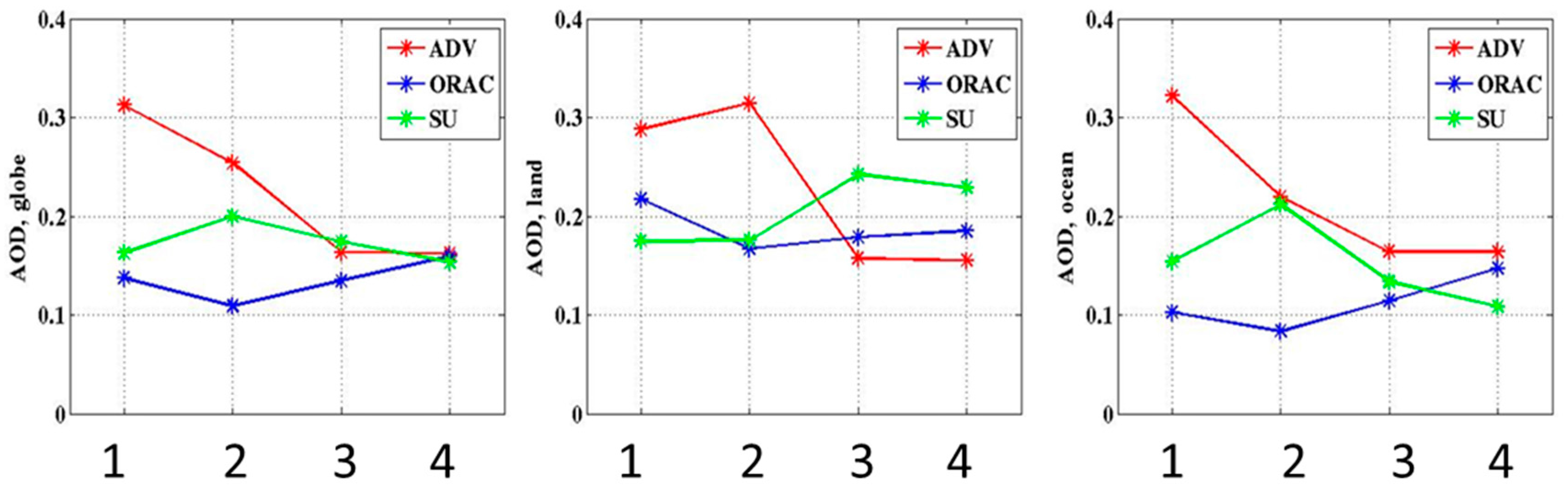
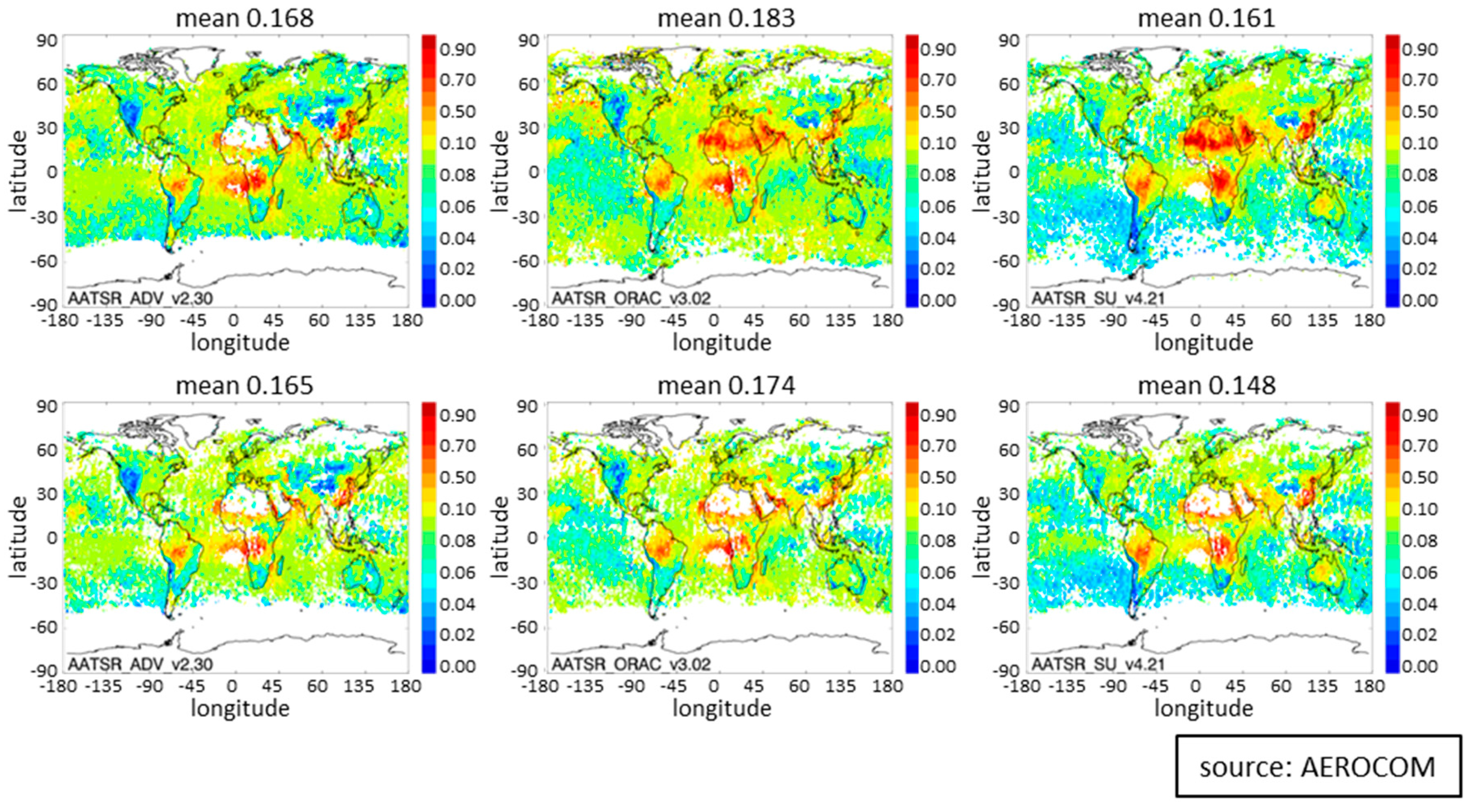
2.5.1. Common Point Evaluation of Gridded L3 Products

Global models typically use gridded daily or monthly datasets. The first step of user assessment of our retrieval products is validation of gridded daily products aggregated from the satellite datasets, matching the nearest satellite 1° × 1° grid cell to daily mean AERONET values. We assess whether this analysis yields different results to the analysis at pixel-level in Section 2.4. In the gridded analysis, the sampling and data gaps inside a grid box are taken into account to evaluate how comparable these datasets are to typical model datasets. A challenge in any retrieval product evaluation is to account for differences in coverage between the retrievals. We show the impact of using a “common data point filter”. The three gridded AATSR L3 retrieval products are compared to daily AERONET sun photometer level 2.0 AOD products (as downloaded from the AERONET website on 21 November 2015) from sites situated below 1000 m height. In order to conduct an “apples-to-apples” comparison, we consider only grid cells where all three retrieval products and AERONET provided a result (i.e., the “common points”). For example, in September 2008 this filtering keeps 71% of the ADV data points in the evaluation, 69% of ORAC and 70% of SU data points.

In Figure 5 the effect of the “common data point filter” is visualized using a quasi-logarithmic color bar to emphasize differences for low AOD values. Due to ADV’s inability to retrieve above bright surfaces, nearly the entire Sahara region is missing from the comparison. The northern part of Siberia is missing due to ORAC. A vital part of the biomass burning outflow region west of Africa is removed because of SU. Parts of the very southern oceans are removed from comparison because of the ADV retrieval. Global mean AOD values are provided on top of each map, demonstrating that the common data point filtering leads to only a small reduction (~0.01) of global averages, which is within algorithm uncertainties. However, the common point filter excludes some interesting cases where only a single algorithm deals with difficult but important regions of the globe.

Table 5. Statistics of L3 evaluation of the three AATSR retrievals against AERONET on common data points for September and the entire year 2008.

Metric	Algorithm
	ADV/ASV v2.30		ORAC v3.02		SU v4.21
	September 2008	All 2008	September 2008	All 2008	September 2008	All 2008
number of points	586	6072	586	6072	586	6072
bias	−0.048 (−26%)	−0.04 (−25%)	−0.001 (−2%)	−0.007 (−8%)	−0.025 (−9%)	−0.021 (−9%)
RMSE	0.12	0.11	0.11	0.11	0.11	0.10
correlation	0.71	0.80	0.74	0.79	0.80	0.83
GCOS fraction	53	52	50	49	60	59

shows a compilation of the resulting statistical metrics. For the “GCOS fraction” we assume an uncertainty in any AERONET measurement of 0.01 here (making the overall criterion: 0.04 or 10%). The analysis is given for two time frames (September 2008 and all 2008), which again agree very well. Comparing the results of Table 5 to those of Table 3 and Table 4, shows that this analysis is consistent with that of Section 2.4.

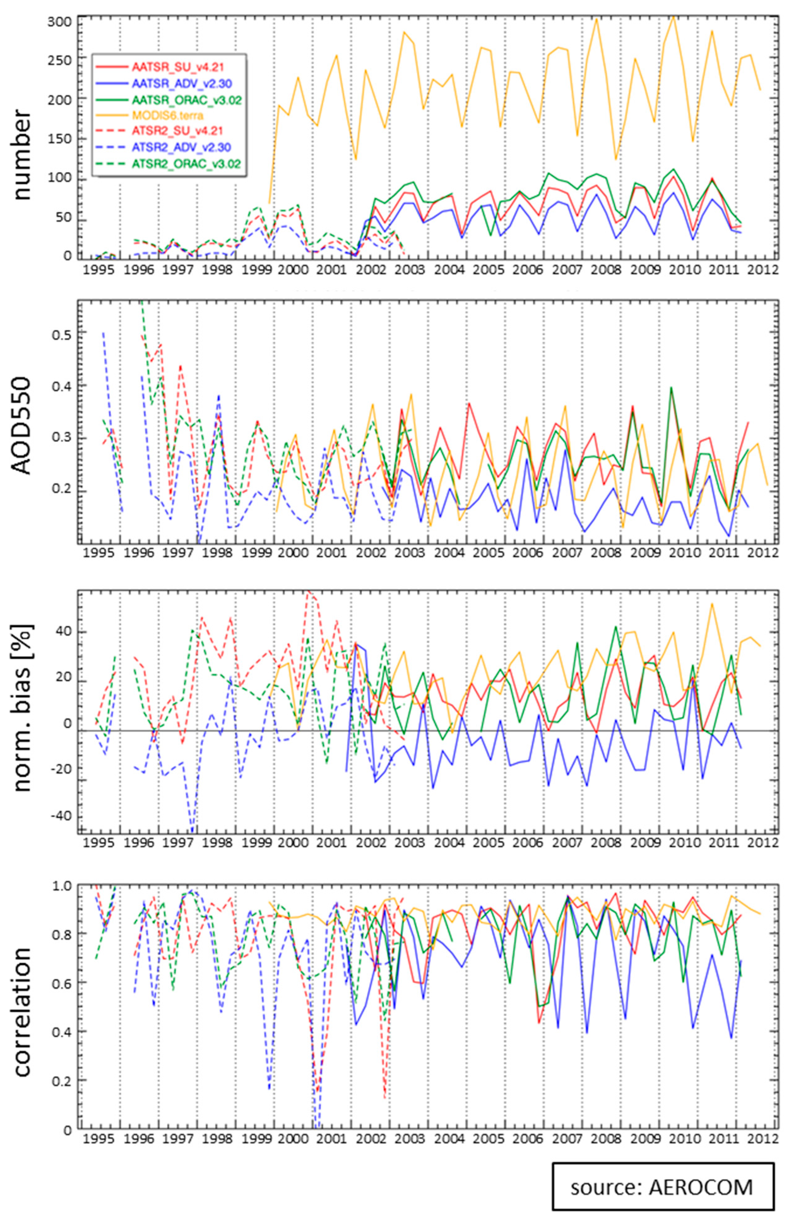
2.5.2. Evaluation of ATSR-2/AATSR Aerosol Optical Depth Temporal Stability

Validating the stability of CDRs is an essential step in proving their suitability for climate applications. This analysis is challenging because the satellite sensors and surface network have evolved inconsistently over time. The ATSR seasonal AOD data record is evaluated by applying AEROCOM tools to derive evaluation statistics based on all daily data points from 1995 to 2012.

Very few AERONET sites were in operation before 2000 (the first five years of the ATSR-2 operation). The following AERONET sites exhibit the longest record: Avignon (Southern France), Banizoumbou (Niger), Bratts Lake (Canada), Capo Verde (Republik Cabo Verde), CEILAPBA (Argentia), GSFC (USA), Sedeboker (Israel) and Lille (Northern France). These are used to evaluate the three 17-year AOD CDRs (ADV, ORAC, SU). We also consider the MODIS Terra collection 6 dataset [38] from 2000. The small number of sites may produce less reliable statistics and limit the ability to represent all global environments. However, this avoids introducing a spatial bias between different years, which would inevitably appear had the entire network been used as it covers more and more regions over time.

In Figure 6 the number of observations within each grid cell is higher by a factor of about 4 for MODIS than for all three AATSR data records (from 2002). This is due to the smaller swath width (also by a factor of 4) of the ATSR instruments compared to MODIS. Figure 6 shows large fluctuation in the number of daily observations at the eight chosen AERONET sites. Four distinct periods can be identified. Before 1999 sun photometer measurements were irregular and sparse. The years 1999 and 2000 provide the best chance to evaluate the ATSR-2 products. MODIS Terra is used from the year 2000 onward to check for any peculiar impact from surface network instability. The stable number of observations after the year 2000 indicates that the 8 sites delivered a rather homogenous data record for validation. The ATSR time series suffers from sensor problems with ATSR-2, limiting the overlap between ATSR-2 and AATSR. From autumn 2002 onward the number of data points available from AATSR per season is mostly constant until mission failure in 2012. Numbers of observations differ among the AATSR retrievals, due to coverage issues mentioned earlier. The second plot in Figure 6 shows the resulting time series of AOD from the three retrievals, split into the ATSR-2 and AATSR record, along with MODIS terra. The inconsistent coverage by the ATSR data records is believed to explain their differences.

The modified normalized mean bias (MNMB, defined as the mean bias divided by the average of the mean satellite AOD and the mean AERONET AOD) in the third plot confirms that most of the time the ADV retrieval shows the smallest values at the selected sites. This is likely related to ADV missing observations in the desert region. Biases for ORAC and SU are correlated, which is most probably due to the fact that they use the same surface model. Comparing 1999 and 2000 MNMB against that of later periods reveals no systematic bias of ATSR-2 against AATSR. Finally, the correlation time series as depicted in the last plot confirm the ATSR-2 and AATSR records have similar quality. Overall, it can be concluded that no instability can be detected in the ATSR-2/AATSR data records. Note, that the MODIS-Terra collection 6 time series shows a slight increase in bias from 2004 to 2012 in Figure 6 (despite of improvements made from the collection 5 to 6 algorithm).

3. Special Aspects of Algorithm Evaluation

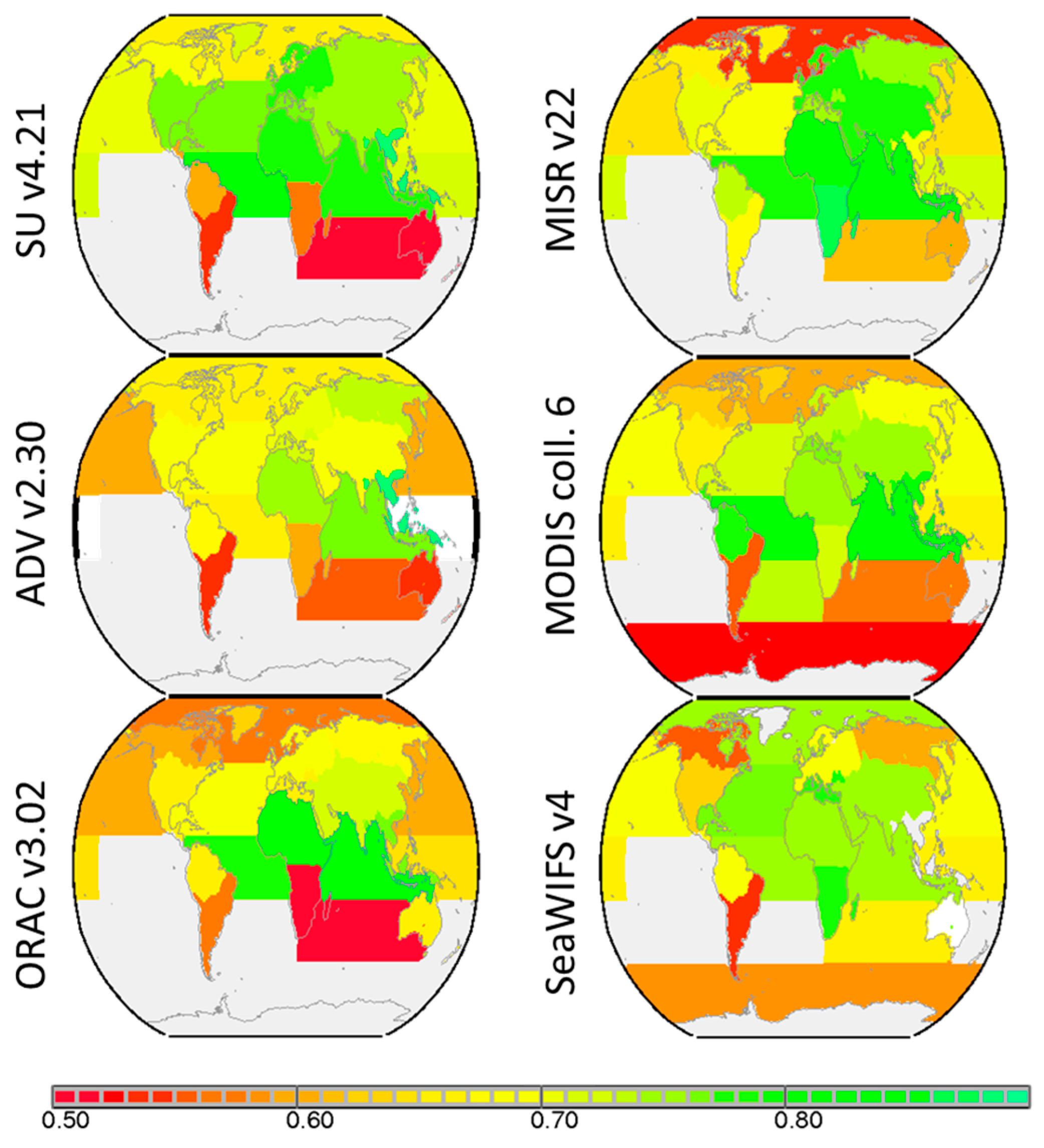
3.1. Assessment of Spatial and Temporal Correlations

A complementary test of the performance of the three ATSR retrievals is the use of skill scores with respect to AERONET and MAN (Maritime Aerosol Network) data. Daily L3 satellite data (of the local time morning overpasses) are compared to AERONET/MAN observations within half an hour of the satellite overpass. To simplify comparisons, all sun photometer data were gridded to the spatial 1° × 1° resolution of the satellite data.

A scoring method (see [20]) has been developed to assess the overall ability of a data record to observe regional and seasonal patterns with respect to trusted reference data. This is done by making the overall score a product of multiple sub-scores. At the smallest (temporal and spatial) scales, bias and correlations are determined and later combined. To minimize misinterpretation due to data outliers, the sub-scoring is based on the relative ordering (or ranking) of values rather than their magnitude and on central statistics (e.g., median, interquartile average and range) instead on general (Gaussian) statistics (e.g., averages and standard deviation).

The total score’s sign indicates the bias direction. For any score, the absolute value ranges from 0 to 1, with 1 being optimal. Statistically meaningful evaluations are often not possible for pre-defined global regions due to retrieval coverage and the lack of reference data. Only regions with successful scores are combined (separately for land and ocean; see

Table 6. Evaluation scores for the three ATSR AOD datasets at 550 nm based on daily L3 “common data point” matches to AERONET data for the year 2008. Total scores are listed in column 2 and the underlying sub-scores for bias, temporal correlation and spatial correlation are presented in columns 3–5.

Algorithm	Total Score	Sub Scores
		Bias	Temporal Correlation	Spatial Correlation
Over Coastal/Ocean Regions
ADV v2.30	−0.74	−0.87	0.84	0.74
ORAC v3.02	+0.73	0.88	0.83	0.77
SU v4.21	+0.75	0.89	0.84	0.77
Over Land Regions
ADV v2.30	−0.68	−0.86	0.80	0.85
ORAC v3.02	+0.70	0.86	0.82	0.86
SU v4.21	+0.73	0.86	0.85	0.87

), globally. The score comparison of Table 6 indicates that the SU algorithm is slightly better over land than ORAC and ADV, particularly in temporal correlations. Over ocean/coastal sites, differences between the three algorithms are small.

In a second step, scores for three different NASA retrievals (Multi-angle Imaging Spectro Radiometer—MISR, version 22, ([39], and references therein); MODIS collection 6 [38] and SeaWiFS version 4 [13]) are included for comparison (Figure 7,

Table 7. AOD evaluation scores for 3 AATSR algorithms and 3 NASA AOD retrievals over land and ocean based on daily L3 matches to AERONET data for the year 2008.

Algorithm	Total Score	Sub Scores
		Bias	Temporal Correlation	Spatial Correlation
Over Coastal/Ocean Regions
ADV v2.30	+0.64	0.82	0.77	0.72
ORAC v3.02	+0.68	0.88	0.77	0.75
SU v4.21	+0.72	0.89	0.81	0.80
MISR v22	+0.71	0.82	0.86	0.81
MODIS collection 6	+0.67	0.81	0.82	0.82
SeaWIFS v4	+0.66	0.89	0.75	0.81
Over Land Regions
ADV v2.30	−0.68	−0.85	0.80	0.82
ORAC v3.02	+0.68	0.87	0.78	0.82
SU v4.21	+0.69	0.86	0.80	0.83
MISR v22	+0.76	0.88	0.87	0.85
MODIS collection 6	+0.73	0.88	0.83	0.78
SeaWIFS v4	+0.70	0.87	0.80	0.78

) as was repeatedly requested by users. Working with six datasets prevents use of a common point filter. As an advantage, skill scores can be calculated for more regions, but the comparability between different datasets is reduced (a regional sub-score can be based on observations of entirely different aerosol episodes).

While land and ocean scores are quite similar, regional skill scores, as illustrated in Figure 7, are quite diverse. Poorer scores usually occur over continents, the Southern hemisphere, the Pacific and higher latitude ocean regions. Many of these low scores are associated with relatively poor statistics. Over land, MODIS and MISR AOD scores are on average better than AATSR scores (mainly due to better temporal correlation scores). Over oceans, AATSR scores are comparable but coverage is also much smaller than MODIS and SeaWiFS. The regional total scores in Figure 7 show that no single ATSR retrieval is better than any other ATSR retrieval simultaneously in all regions (with available scores). Over oceans the MISR retrieval scores surprisingly well, despite its known positive biases for low AOD values there. It should be noted that many regions where the MISR bias is relatively large do not contribute to the MISR ocean total score.

3.2. Assessment over a Special Region with Sparse Standard Reference Data (AOD over China)

In order to validate the new ATSR AOD records over mainland China, where AERONET data are sparse, we compare to data from the China Aerosol Remote Sensing Network (CARSNET) for 2008. AERONET sites in China are limited in number and most are located in eastern China. Most collocated pairs are in March to November with few in winter. The combination of AERONET and CARSNET alleviates issues from the small numbers and uneven distribution of AERONET sites.

CARSNET uses the same type of instrument as AERONET. The total uncertainty in its AOD values is about 0.01 to 0.02. Five CARSNET sun photometers were calibrated at the global observatories which are the master calibration sites for AERONET. These instruments were then installed at the Beijing-CAMS site (39.93N, 116.32E, which is operated for both CARSNET and AERONET), and they were used as masters to inter-calibrate all field CARSNET instruments at least once a year, following the AERONET calibration protocol [40]. A comparison between the AODs calculated with the CARSNET procedure vs. AERONET results showed that the AOD values at visible wavelengths were about 0.01 larger than those from AERONET; correlation coefficients were larger than 0.999 and had a 99.9% significance level. Thus, the sets of results from the two networks are highly consistent with one another.

The validation results for the three AOD products over China are shown in

Table 8. Validation of AATSR L2 AOD products (ADV, ORAC and SU) with ground-based data in China for the year 2008 (AERONET alone, AERONET and CARSNET).

Metric	Algorithm
	ADV/ASV		ORAC		SU
	AERONET	AERONET + CARSNET	AERONET	AERONET + CARSNET	AERONET	AERONET + CARSNET
number of points	50	307	66	612	57	435
bias	−0.08	−0.15	0.03	−0.06	−0.03	−0.12
RMSE	0.09	0.12	0.19	0.21	0.09	0.14
correlation	0.92	0.79	0.72	0.47	0.91	0.82

. Using reference data from both networks changes the evaluation results compared to using AERONET alone. The SU and the ADV products have higher accuracy but less coverage, while the ORAC product has more coverage at the cost of accuracy. The performances of SU and ADV products are similar with correlation coefficients of about 0.8–0.9 and RMSE (Root Mean Square Error) within 0.15. The analysis included high AOD values (AOD > 1). The SU algorithm retrieves more high AODs than ADV, leading to more validation matches. All algorithms tend to underestimate AOD to some degree. Scatter plots (not shown) indicate that the underestimation gets more severe with larger AOD.

3.3. Validation of Pixel-Level Uncertainties

Uncertainty is a vital component of any dataset for climate applications as it provides the context with which to understand the quality of the data and how it compares to other measurements. As highlighted in Figure 1, validation against independent observations is a fundamental step in the development of a dataset. This applies equally to assessing the capability to predict pixel-level uncertainties which are contained in the datasets. The validation of uncertainty is not frequently discussed, but without it there is little reason to trust the uncertainty values produced. To validate uncertainty, it is necessary to demonstrate that it provides a useful representation of the distribution of error. Technically, the “true” value of AOD will never be known and so the error cannot be specified exactly. Direct-sun observations of AOD from the AERONET sun-photometer network are substantially more accurate than those produced by satellites as they suffer fewer sources of error (e.g., there is no influence from the surface, the impact of multiple scattering is minimized using a long baffle). By neglecting the uncertainty in AERONET observations and possible issues with their ability to represent a satellite pixel area, the error in the retrieval can be approximated by the difference between the satellite and AERONET retrievals (herein referred to as “error”).

To evaluate how well the standard uncertainty σ_ATSR represents the observed distribution of error, we consider the metric

$$∆ =\frac{AO{D}_{\text{ATSR}}-AO{D}_{\text{AERONET}}}{{\sigma }_{\text{ATSR}}}$$

For one pixel, a standard uncertainty σ_ATSR (which is contained in the level2 files for each pixel) implies that we expect the errors AOD_ATSR − AOD_AERONET to have a Gaussian distribution with a standard deviation of σ_ATSR. A non-zero mean of Δ indicates the presence of residual systematic errors (which may be resolved in future algorithm development). A standard deviation of Δ greater than one indicates that uncertainties are underestimated, which could result from neglecting an important source of error. On the other hand, a standard deviation less than one indicates an overestimate. AERONET data has been cloud filtered (in a different manner to the satellite observations). The comparison will only represent the subset of environments that contain an AERONET station (e.g., a consistently poor retrieval over remote mountainous regions would not be identified by this validation) and that have a high probability of being cloud-free. If Δ is normally distributed, 68.3% of values should fall within the range [−1,+1]. If the fraction is smaller, uncertainties are underestimated; if it is larger, uncertainties are overestimated.

Such a validation has been performed for all three ATSR algorithms over the full 17-year period using collocations with AERONET (retrievals centred within 50 km radius and 30 min interval of a valid L2 observation at any site). For brevity, only the results of the SU algorithm are discussed here. Considering their histograms, the estimated uncertainty had a substantially fatter tail than the observed error in the earlier version. In response to this evaluation, the treatment of uncertainty in the algorithm was revised and the validation was repeated. The revised uncertainty appears to be a more accurate representation of the error, with ~60% of values falling within the range [−1,+1]. Uncertainties better reproduce the distribution of error over land than at coastal sites. This is not surprising since these regions will contain mixtures of land and water, which will be poorly represented, and coastal waters are difficult to model as they tend to be shallow and contain sediments. The histogram of absolute values of uncertainty (Figure 8) shows that v4.21 contains a good reproduction of the observed error, though it contains an excess of very small values. The comparison of the earlier version with the newest version confirms that the iterative evolution cycle has led to enhanced ability to estimate pixel-level uncertainties. This represents an important achievement in addition to improving AOD retrieval accuracy.

The stability of the ability of the uncertainty to represent the distribution of error is evaluated in Figure 9. The fraction of the points where the ratio Δ falls within [−1,+1] shows that this version presents a sensible representation of the error over land throughout the 17-year record. The underestimation of coastal uncertainty exhibits greater variability, indicating the sources of error omitted from the current uncertainty estimate are more likely to be transient, such as data coverage, rather than a relatively consistent feature, such as the incorrect modelling of shallow waters. We remind the reader that for the early part of the ATSR-2 period there were many fewer AERONET sites.

4. Application of the Cyclic Approach to Other Complementary Aerosol Datasets

The analysis of further satellite aerosol datasets with complementary information content is necessary so that all relevant aerosol information as requested by GCOS and AEROCOM can be obtained and validated globally. Accordingly, we extend our description to four more aerosol datasets. Note, that it is not our intention to describe the full analysis of each dataset in this paper. We aim rather at showing the transferability of our iterative user-driven approach and at illustrating one additional aspect of the evolution cycle with each of them. We start with a CDR evaluation by polarization satellite retrievals in regions with few ground-based data. We consider the evaluation of aerosol properties such as dust or absorption by evaluating thermal infrared and UV measurements. For aerosol extinction profiles we analyze star occultation observations. The datasets and algorithm characteristics of those four studies are summarized in

Table 9. Overview of further data sets and algorithms discussed in this paper.

Vertical	Parameter	Sensor(s)	Coverage, Resolution	Algorithm, Version	Characteristics	References
Total column	AOD 0.55 µm + several aerosol/surface properties	POLDER/PARASOL	2008 selected regions 6 × 6 km, ~weekly 1° × 1° daily/monthly	Principle: polarization, multi-angle, multi-spectral radiometer in the visible
				GRASP V0.07	multi-pixel aerosol/surface retrieval, smoothness constraints	[41,42,43,44,45]
					land surface: bi-directional reflectance/polarization models	[46,47]
					ocean surface: water-leaving radiance model	[48]
					aerosol model: spheroidal kernels	[43]
					cloud mask: POLDER cloud mask	[49]
	Dust AOD 10 µm, 0.55 µm	IASI	2013 Global dust belt 12 km, twice daily 1° × 1° daily/monthly	Principle: thermal infrared spectrometer
				IMARS V4.2	Spectral pattern recognition	[50]
					land/ocean surface: 24 example emissivity spectra	[51]
					aerosol model: Asymptotic Approximation Approach	[52]
					cloud mask: probability based a posteriori cloud filtering
				LMD V1.3	Look-up table	[53]
					surface temperature co-retrieved with AOD and altitude
					land surface: monthly grid of IASI surface emissivity	[54]
					aerosol model: Mie calculations, fixed size distribution	[55]
					cloud mask: threshold filtering during inversion process	[56]
				MAPIR V3.0	Optimal Estimation (dust profiles and surface temperature)	[57]
					land surface: emissivity from Zhou et al.	[58]
					ocean surface: emissivity from Newman et al.	[59]
					aerosol model: spherical, Reff 2 µm, HITRAN refract. index	[60]
					vertical profile: a priori	[61]
					cloud mask: IASI level2 (max 10%)
				ULB V5.0	Neural network	[62]
					Surface emissivity database	[58]
					CALIPSO dust altitude climatology aerosol model: spherical	[63]
					lognormal, preset refractive indices	[64]
					cloud mask: IASI L2 (Eumetsat), 0% threshold
	Absorbing Aerosol Index AAI	TOMS GOME SCIAMACHY GOME-2 OMI	1978–1993 1995–2003 2002–2012 2007– 2004– 1° × 1° daily/monthly	Principle: UV spectrometer, ratio of two UV wavelengths
				AAI V1.4.7	index based on 2 UV reflectances	[65]
					compared to simulated Rayleigh reflectances
					Wavelength pairs: 340/380 nm (GOME(-2), SCIAMACHY), 331/360 nm (TOMS) and 354/388 nm (OMI)
					Sensitivities: mostly aerosol concentration and height
					Degradation correction	[66]
					No cloud masking needed
					sun glint and solar eclipse filtering
Vertical profile	Aerosol extinction 0.55 µm	GOMOS	2002–2012 Global 2.5° × 10° Monthly 5° × 60° 5 daily	Principle: Star occultation spectrometer in the UV, visible, and NIR
				AERGOM V2.14 V2.19	vertical extinction profiles in the stratosphere	[67,68]
					estimate of stratospheric AOD	[69]
					Wavelengths: 300–750 nm; (so far at 550 nm)	[70]
					Polar stratospheric clouds (PSC) and subvisible cirrus clouds	[71]

.

While the more mature algorithms (GOMOS—Global Ozone Monitoring by Occultation of Stars, AAI—Absorbing Aerosol Index) have been developed and evaluated in parallel with the ATSR CDR, the cyclic evaluation of further algorithms (POLDER—POLarization and Directionality of the Earth’s Reflectances, IASI—Infrared Atmospheric Sounding Interferometer) has started later. In all cases, an iterative approach with repeated algorithm development and evaluation by an integrated team of developers and users as shown in Figure 1 is applied. In three cases only one algorithm is applied, whereas for IASI again an ensemble of four algorithms is compared. For later cycles (e.g., IASI), lessons learned from the earlier rounds (ATSR, GOMOS) were taken into account, which enabled faster progress already during the round robin exercise step. We summarize those activities here, to demonstrate the general applicability of the evolution cycle proposed.

4.1. Qualifying a Satellite Dataset as Quasi-Reference (POLDER GRASP AOD and Aerosol Properties)

Validation requires suitable ground-based reference data. Where AERONET has sparse coverage, validation remains difficult. Here an alternative solution is suggested: use another satellite dataset as a quasi-reference. To be useful, this quasi-reference needs to exhibit a higher accuracy than the satellite datasets under validation. With the highest information content (polarization, multi-angular, multi-spectral) the POLDER instrument is the best candidate to produce such a reference dataset. Here we discuss the validation of the new multi-pixel GRASP (Generalized Retrieval of Aerosol and Surface properties) algorithm over land applied to POLDER/PARASOL data in data-sparse regions around one selected AERONET site, each. However, GRASP provides also valuable capability to retrieve additional aerosol properties, such as absorption and size.

Table 10. Comparison of GRASP/PARASOL AOD and SSA at 670 nm vs. AERONET over Mongu, Banizoumbou, IER_Cinzana, Agoufou, Ilorin sites in Africa for 2008 with two different “fitting residuals” of 7 % and 3 %. Green colors indicate improvement for lower fitting residuals.

Metric	Parameter/Quality Control
	AOD670/7% Fit Residual	AOD670/3% Fit Residual	SSA670/7% Fit Residual	SSA670/3% Fit Residual
L2 Validation (Pixel Window, Time Window, All Points)
number of points	455	182	233	100
bias	0.02	0.05	−0.01	0
RMSE	0.18	0.14	0.06	0.04
correlation	0.88	0.95	0.65	0.72

shows the dependence of the quality of GRASP retrievals on the degree to which they fit the top of atmosphere measurements (“fitting residual”). As can be seen from the table, more accurate fitting of PARASOL multi-angle, multi-spectral photo-polarimetric measurements secures more accurate retrieval.

GRASP aerosol retrievals from POLDER/PARASOL (with a “fitting residual” threshold of 3%) in several geographical zones are then validated against AERONET data. The summary of those comparisons is shown in

Table 11. Comparison of GRASP/PARASOL AOD at different wavelengths, Ångström exponent (AE) and single scattering albedo (SSA) vs. AERONET over sites in Africa (Mongu, Banizoumbou, IER_Cinzana, Agoufou, Ilorin) and over Beijing and Kanpur for 2008. Values are covering high extremes (AOD: 0–4, AE: 0–2.5, SSA: 0.73–1.0).

Metric	Parameter
	AOD440	AOD670	AOD865	AE (670–865)	SSA670	SS865
Over African Sites
number of points	182	182	182	157	100	100
bias	0.004	0.05	0.04	0.03	0	0.01
RMSE	0.14	0.14	0.14	0.18	0.04	0.04
correlation	0.96	0.95	0.95	0.91	0.72	0.76
Over Beijing and Kanpur
number of points	58	58	58	56	21	21
bias	0.03	0.01	−0.002	0.04	0.01	0.02
RMSE	0.25	0.18	0.14	0.28	0.06	0.06
correlation	0.97	0.96	0.95	0.86	0.55	0.67

and Figure 10: GRASP aerosol retrievals are in a good agreement with AERONET observations, the correlation coefficients are substantially higher over land than those of the ATSR retrievals (see Table 3) and RMSE values are similar to them; furthermore, SSA is available with similar quality. To understand the strength of the validation shown in Figure 10, it is important to note that the AOD extends to values which are much larger than for AATSR in Figure 2. Furthermore, in Africa, difficult bright surfaces are included among the reference sites. This means that those RMSE values are also of highest quality.

These results suggest that the GRASP algorithm can provide robust extended aerosol characterization over diverse land cover areas including very bright surfaces. Although GRASP does not reach the quality of AERONET, it is overall better than ATSR and can thus serve as quasi-reference for validating ATSR retrievals in absence of AERONET. It should be noted that so far no global full mission CDR was processed with GRASP due to the large computing resources needed.

4.2. Round Robin Exercise for Dust AOD from Thermal Infrared Measurements by IASI

In this section, dust AOD derived from a thermal infrared spectrometer (IASI) by four different algorithms (Table 9, acronym list in the appendix) is analyzed in a round-robin exercise. This responds to one of the AEROCOM required variables. The IASI instrument is a Michelson interferometer operating in the thermal infrared (TIR) spectral range with a high spectral resolution (0.5 cm⁻¹ after apodization) and a ground resolution of 12 km at nadir. Desert dust has a clearly identifiable extinction signal in the TIR window range caused by vibrational resonance peaks of silicates (e.g., [72]. Consequently, it is possible to retrieve dust AOD from IASI, together with other dust properties such as altitude, particle size and dust composition. Moreover, the infrared domain allows observation over bright desert surfaces, where many retrieval algorithms in the solar domain are not well suited [73]. A drawback is the limited sensitivity of TIR observations near the surface. Finally, both day and night observations provide information on diurnal variations of dust loadings as unique inputs for models.

The four retrieval algorithms are largely different as characterized in Table 9. For the first time the independent European groups working on TIR aerosol retrieval were brought together for a round robin exercise of IASI dust AOD. This round robin exercise assesses the state of the TIR retrieval development and sets the stage for subsequent algorithm evolution cycles. Already in preparation for this first-ever IASI aerosol round robin exercise iterative algorithm development and validation was conducted and led to important dataset improvements. For the round robin exercise, one year of data (2013) has been processed with all four algorithms for a region covering the major dust source and outflow (from 80°W to 120°E and from 0°N to 40°N). This data volume was chosen based on that used in the round robin exercise for AATSR but adapted to the differing IASI characteristics: wider swath (~2000 km), geophysical focus of dust observations in the selected region, 12 months of data, slightly larger pixel size (12 km vs. 10 km ATSR super pixels).

For independent validation, AERONET data are used as “ground truth” for dust AOD. However, AERONET does not provide dust AOD. Consequently, coarse mode AOD at 0.55 µm from the AERONET direct-sun spectral deconvolution algorithm (SDA) product is used as a proxy for desert dust, even though it does not always represent desert dust. Additional filtering for small Ångström exponent (AE) was tested, but did not introduce major changes (except reducing data amounts significantly). Another problem arises from the conversion of the IASI AOD values from infrared to visible wavelengths. This is not trivial since an accurate knowledge of both composition and particle size is required but is not available [51,53]. The conversion factors used for the different algorithms are bound to strong approximations which introduce additional uncertainty into the converted dust AOD at 0.55 µm. Due to the different retrieval approaches, it is not possible to use the same conversion factors for all four algorithms.

The validation against AERONET is conducted with daytime (descending orbit) IASI data over L2 (satellite pixels) and L3 (gridded daily one degree) datasets. Figure 11 presents the scatter density plots and difference histograms vs. AERONET coarse mode AOD for the L2 comparison of the four algorithms, whereas

Table 12. Validation of IASI AOD at 550 nm for the four datasets (L2 and L3) against AERONET SDA coarse mode AOD at 550 nm for the region 80°W to 120°E and from 0°N to 40°N over the whole year 2013 for L2 (satellite projection) and L3 (gridded) datasets.

Metric	Algorithm
	IMARS v4.2	LMD v1.3	MAPIR v3.0	ULB v5.0
L2 Validation (Pixel Window, Time Window, All Points)
number of points	4408	4972	3141	5053
bias	−0.08	−0.01	+0.28	+0.02
RMSE	0.14	0.12	0.40	0.12
correlation	0.45	0.60	0.41	0.80
L3 Validation (Gridded, Daily; Common Points)
number of points	2652	2652	2637	2652
bias	−0.08 (−67%)	−0.05 (−38%)	+0.12 (+94%)	+0.01 (+8%)
RMSE	0.16	0.12	0.28	0.12
correlation	0.40	0.66	0.47	0.76

shows the L2 and L3 comparisons to AERONET.

It can be seen that there are substantial differences between the algorithms. The ULB and LMD results tend to be similar and closer to AERONET than those of IMARS and MAPIR (under and overestimating dust AOD, respectively). Additionally, the differences in coverage/number of validation points become obvious. The reliability of the validation results is documented by the fact that the analysis of L2 and L3 data show similar tendencies for each algorithm. For all algorithms, further algorithm development and evaluation is needed to come closer to the user requirements as stated in Table 2. Currently, the full 10 year IASI records are processed using further improved algorithm versions based on the validation results of the round robin exercise. As we had learned with the ATSR algorithms after their round robin exercise, no single algorithm is perfect; the evolution cycle is continued with all four algorithms. Ultimately, different dust AOD datasets from entirely different sensors and retrieval algorithms for IASI, AATSR and POLDER will be inter-compared.

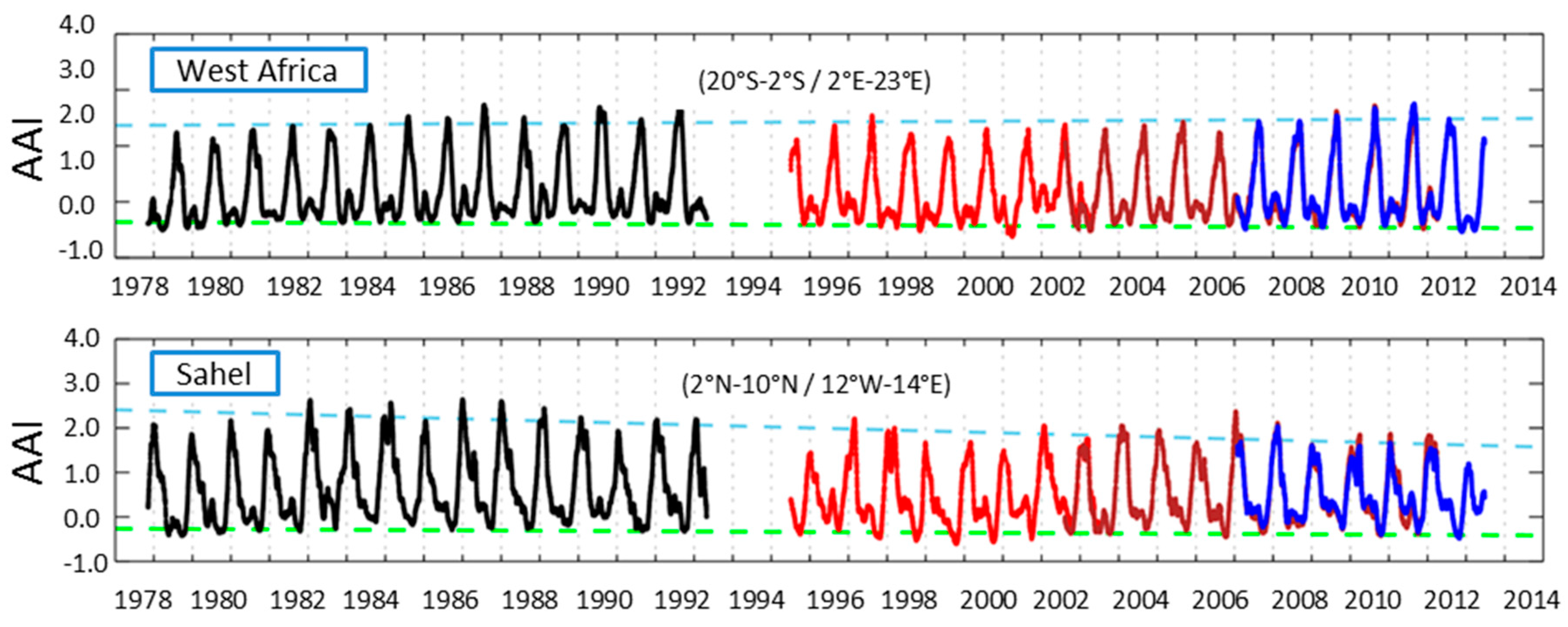
4.3. Evaluating a Time Series of a Qualitative Data Record for Absorption (AAI)

Here, we discuss the use of a qualitative multi-sensor 35-year data record to study absorption, a variable required by GCOS. The absorbing aerosol index (AAI) is a qualitative index based on Earth reflectance measurements performed at two UV wavelengths [65,74]. The AAI from 1978 until present from five different satellite instruments (TOMS, GOME-1—Global Ozone Monitoring Experiment, SCIAMACHY—Scanning Imaging Absorption SpectroMeter for Atmospheric CHartographY, OMI, and GOME-2 ) is the longest global dataset on aerosol absorption. The five individual sensor datasets can be merged after extensive calibration efforts (e.g., pre-processing correction on the Earth reflectances, [66]). The OMI instrument shows very small instrument degradation and therefore does not require any stability correction.

In Figure 12 we present time series of regional mean AAI for two frequently studied desert dust and biomass burning aerosol regions. The OMI AAI time series is not plotted because it overlaps largely with the other AAI time series. A first impression is that seasonal variations are captured by all of the AAI data records for all regions, and that there are no obvious inconsistencies in and between the AAI data record parts.

For discussion we focus on the first time series, labeled “West Africa”. This biomass burning area with relatively small year-to-year variability is ideally suited for studying the integrity and consistency of the various AAI time series. There is good consistency between the GOME-1 and SCIAMACHY AAI in the overlapping time period (August 2002–June 2003) and also between the SCIAMACHY and GOME-2 AAI (January 2007–April 2012). Minima in the seasonal variation occur in months when biomass burning is minimal. A best linear fit through the annual minima is shown by the dashed green line. The calculated trend is −0.003 ± 0.005 index points per year, which corresponds to a total decrease of 0.1 ± 0.2 index points for the entire time period. This is a small trend compared to the estimated accuracy of the method that was used to correct for instrument degradation (errors less than 0.1 index point, see[66]) and the estimated error on the trend is larger than the apparent trend itself. Also for five other regions no significant trend in the aerosol minima (background conditions) was detected. This indicates that the multi-sensor AAI data record has good stability.

Based on this background stability, we investigate the use of AAI time series for studies of trends in the presence of aerosol. To do this, we calculate the best linear fit of annual maxima. For the biomass burning region “West Africa” no significant trend is noticeable (+0.12 ± 0.2 change over the full period). Similar small values (−0.20 ± 0.2, and −0.06 ± 0.2), respectively, were calculated for regions “Rice straw burning” (18°N–28°N, 100°E–120°E) and “Amazonia” (27°S–5°S, 66°W–52°W). We conclude that the selected biomass burning regions do not show a significant trend in the presence of aerosol which is in agreement with other findings (e.g., [75]).

The second region “Sahel” is mostly dominated by desert dust aerosol types (native and/or by transport). The maxima trend analysis reveals a significant AAI reduction of −0.79 ± 0.2 over the 35 years. Further dust-dominated regions “Sahara” (19°N–31°N, 7°W–15°E) and “North Atlantic Ocean” (8°N–25°N, 52°W–17°W) show similar reductions of −0.42 ± 0.2 and −0.64 ± 0.2, respectively, over the 35-year period. This decreasing AAI trend in the presence of aerosol in dust regions is in agreement with other studies (e.g., [75]).

Since the AAI itself is a qualitative index, it must be kept in mind that it is sensitive to aerosol concentration but also to the height of the aerosol thus making its direct interpretation somewhat difficult. Nevertheless, it may be very useful for qualitative comparisons with aerosol presence in global atmospheric chemical transport models. An AAI simulator, which is meant to bridge the gap between AAI and (A)AOD (Absorbing Aerosol Optical Depth) and to fully exploit the information content of the AAI, is currently being developed. Serving as input for this AAI simulator, the multi-sensor AAI data record can act as an important independent reference for the behavior of chemical transport models, especially for the earlier years which are currently not covered by satellite measurements of (A)AOD. We conclude that the multi-sensor AAI record is a consistent time series resulting from a stable (re-)calibration covering a 35-year time period. Its analysis is particularly meaningful in regions of rather homogeneous conditions.

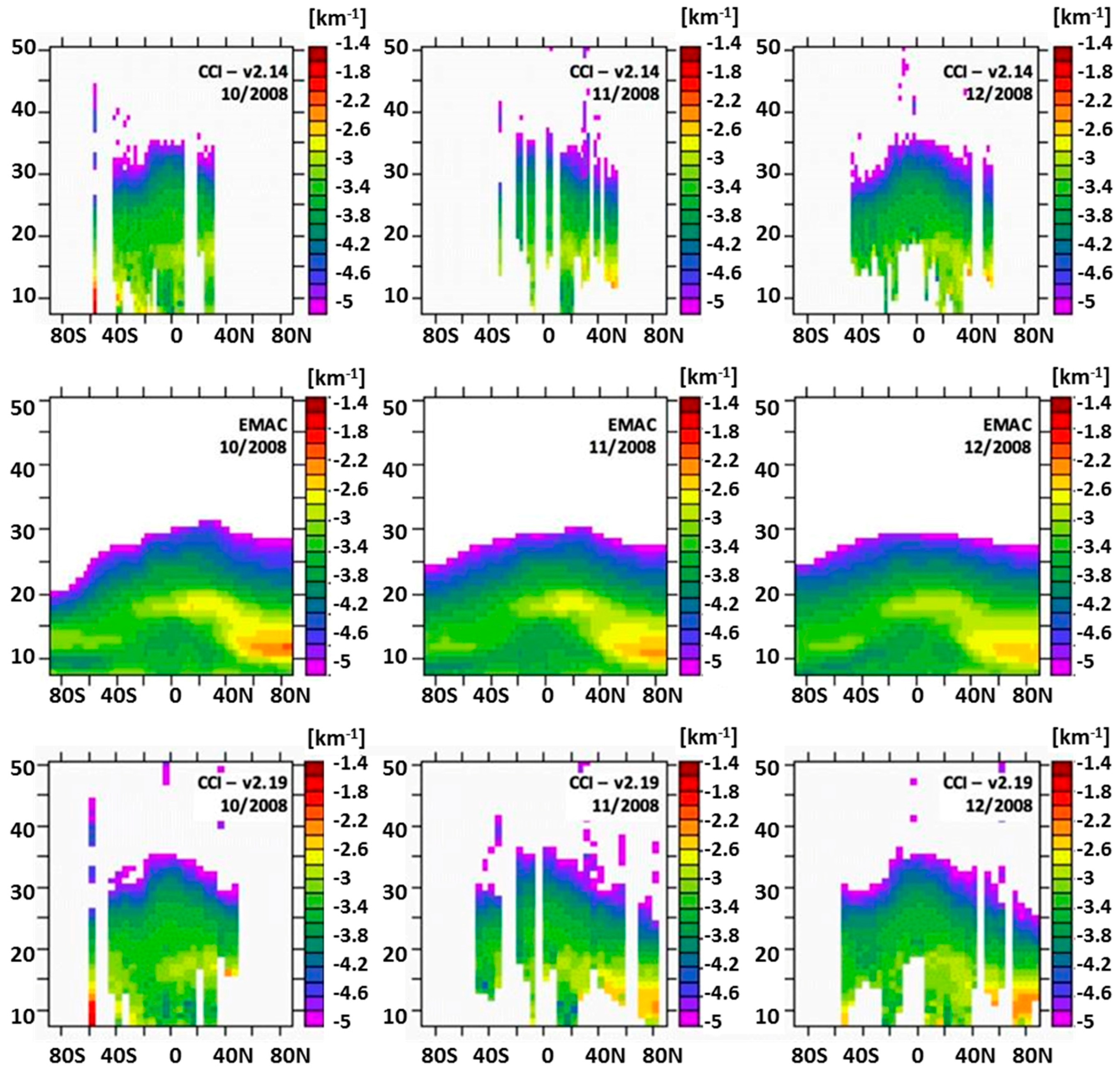
4.4. Iterative Optimization of Product Resolution to Quantify Stratospheric Extinction Profiles (GOMOS)

Finally, we consider a 10-year stratospheric extinction profile CDR to evaluate the vertical coverage of aerosol, as requested by GCOS. GOMOS onboard ENVISAT used the stellar occultation technique to measure transmission spectra from the Earth’s limb in the UV-Vis-NIR (ultraviolet, visible, near-infrared) spectral range. The stratospheric product used here is generated from AerGOM (GOMOS Aerosol Profile Information Retrieval Prototype Processor Development) extinction profiles [70,71]. In order to reduce the noise and to increase the quality of the stratospheric extinction, a subset of occultations are averaged. Accordingly, unlike the tropospheric products, a L3 gridded dataset of several parameters is provided: aerosol extinction and AOD at 550 nm, and their spectral dependence (expressed by the Ångström exponent). Each variable is also accompanied by its associated uncertainty. After several evolution cycles, the stratospheric products are currently available in two versions with different spatial and temporal resolutions. We discuss here the importance of the close interaction with users to take the right decisions in optimizing a CDR during the iteration.

A modeling group evaluated the stratospheric product as a basis for comparison with their model EMAC (ECHAM/MESSy Atmospheric Chemistry model, [76]). In this model the main source for background stratospheric aerosol is the oxidation of carbonyl sulfide (COS). It also includes all known major, small to medium scale explosive volcanic eruptions where the plume reached the stratosphere or the upper troposphere with an injected SO₂ mass above 14 km exceeding 15 kt. The volcanic SO₂ injections have been estimated from the NASA SO₂ database and MIPAS (Michelson Interferometer for Passive Atmospheric Sounding) onboard ENVISAT observations [77]. To compare with the observations, aerosol extinction is derived from the model and calculated from Mie theory using pre-calculated look-up tables for six aerosol components: water, water-soluble species (including sulfuric acid and sulfate aerosol), organic carbon, black carbon, mineral dust, and sea salt in the Aitken, accumulation, and coarse modes.

A comparison of the EMAC model and the GOMOS product was initially done for 2008; results are shown for the last 3 months in the upper and middle panels of Figure 13. The volcanic sulfate aerosol from the Kasatochi eruption (52°N) was visible in both GOMOS data and the model results in the northern hemisphere near the tropopause (maxima at the right side of the monthly plots). In the middle stratosphere the satellite extinction product was larger than in the model pointing to neglected extinction of meteoric dust in the model.

A detailed examination led to a set of user recommendations guiding further algorithm development without compromising product quality by including the treatment of more difficult measurements. Sparse coverage, particularly at high latitudes, should be improved in addition to the removal of undesirable negative extinction values. It was also recommended to flag rather than filter polar stratospheric clouds (PSCs). Finally, it was suggested that a finer temporal resolution be made available, as the monthly means used in the early versions were often not sufficient to observe small to medium scale volcanic events. In response to this assessment, an improved data record has been produced. The selection of purely dark limb observations has been relaxed to partly include observations in twilight situations (solar zenith angle >105°), improving the coverage at high latitudes without impacting significantly the product quality. A more refined selection of profiles improved the negative extinction issues. In addition, coverage was improved near the polar regions by changing the limitations on solar zenith angle. Finally, a different spatio-temporal resolution has been made available in addition to the original monthly product: a 5-day resolution data record aimed at better capability to follow smaller volcanic eruptions or rapidly evolving dynamical patterns, though the spatial resolution had to be adjusted to ensure a sufficient number of profiles per bin. All these changes increased the coverage and detail in the dataset while not decreasing its accuracy. The lower panels in Figure 13 illustrate the improvements made to the data record using the latter version with high temporal resolution (version 2.19), especially compared with the previous results (version 2.14) presented in the upper panels. Both data records now span the entire ENVISAT mission between 2002 and 2012.

Analysis of the new product by the users confirms that it is suitable for the observation of volcanic eruption signatures which were not visible in the previous grid. In particular, the GOMOS data record is able to provide data in spatio-temporal regions which were insufficiently covered by other space experiments (MIPAS, OSIRIS - Optical Spectrograph and InfraRed Imager System, etc.). This constitutes a highly valuable data source to describe the injection of aerosols from volcanic eruptions into the upper troposphere and the stratosphere. The 10-year ENVISAT data record is sufficiently long to contribute to the detailed inventory of volcanic emissions behind the observed increase of aerosol burden since 2000 [76,78]. A detailed description of this contribution will be the subject of a future publication.

5. Conclusions

This paper summarizes the lessons learned (scientific and programmatic) during algorithm development and evaluation cycles for aerosol Climate Data Records (CDRs) during the ESA Aerosol_cci project. This is (so far a 5 year) collaboration of much of the European satellite remote sensing community with 18 partner institutions and several external contributors. Having worked on the iterative development and evolution of five different satellite aerosol CDRs with different maturity we can draw general conclusions. We demonstrate the benefit of such a collaborative approach with one of our most mature datasets (three ATSR 17-year CDRs). Furthermore, we highlight important aspects of dataset evaluation with the ATSR CDRs and other four records which contain complementary aerosol information. Through the steps outlined in this paper, we demonstrate a practical implementation of the GCOS climate monitoring principles [6] that is relevant to algorithms and datasets (in the following we identify numbered GCOS principles as GCOS-NN in brackets).

Firstly, new algorithm versions must be fully validated (GCOS-1 new systems or changes). Validation needs to be comprehensive and take sampling limitations into account (GCOS-4 regular assessment, GCOS-8, GCOS-b and GCOS-11 appropriate sampling). This is done by calculating statistics at a global scale (separately for land and ocean in the case of tropospheric aerosols) complemented by seasonal and regional statistics (as shown in the scoring analysis of ATSR AOD). It can only be applied where sufficient reference stations observe fairly homogenous conditions. When comparing different algorithms, it is recommended to analyze both all points independently (to look at maximal coverage) and only those points observed by all data sets (a “common point” filter) to ensure a like-for-like comparison. The two comparisons will produce different results and need to be interpreted with care but provide additional insight into the strengths and limitations of each algorithm. For validation using ground-based point measurements, there are potential issues regarding the representativity of the reference observations as, by selecting collocated cloud-filtered sun photometer data, an additional cloud clearing is implicitly included. Thus, the validated satellite dataset may be of better quality than the total dataset.

Validation of the datasets needs to be fully transparent and documented (GCOS-3 metadata and documentation)—the CCI documentation standards (followed in this paper) provide a framework to achieve this. For example, the limitations of validation described above need to be clearly stated for users. For credibility, validation must be done by independent experts not involved in algorithm development. If any selection of algorithms is envisaged, the selection criteria need to be defined and agreed in advance. Criteria include typical statistical quantities, visual appearance of maps and quantitative evaluation of the capacity to monitor spatial and temporal features. Furthermore, coverage in space and time of important regions needs to be considered.

For long time series, an assessment of stability is mandatory (GCOS-2 and GCOS 12 overlaps and consistency). This requires reference datasets to be available over the whole period, which becomes more unlikely the further into the past the assessment extends (despite GCOS-6 and GCOS-19 requesting uninterrupted operation and maintenance of complementary in situ data). Limiting validation to stations with AOD measurements throughout the satellite time series restricts the analysis to Europe and North America but this remains a useful assessment of systematic instability of the sensors and algorithms in a variety of retrieval conditions. In addition, the consistency of a time series should be assessed, for example by evaluating the trend over areas where no trends are expected (shown here for the AAI) or in overlapping periods of subsequent sensors (demonstrated for the ATSR instruments and AAI).

Whenever a sufficient amount of reference data is available, validation should be done both at the data’s native resolution and with daily gridded datasets as often used by the modelling community (to account for differences in sampling, GCOS-b and GCOS-11 appropriate sampling). The analyses in this paper were typically unaffected by using L2 or L3 data. Since the information content of an aerosol retrieval depends on the aerosol loading, validation should be stratified into different AOD ranges.

With our iterative algorithm development and evaluation cycle, we have learned several new lessons. We recommend that any CDR generation uses an open development team with retrieval experts, independent validation partners and core users working together within an iterative development and assessment cycle. The cycle starts with addressing user requirements specific to the desired application followed by algorithm development towards those needs, independent validation of the results and user evaluation of the products’ fitness-for-purpose. Algorithm development may involve algorithm experiments to understand critical sensitivities and round robin exercises to assess the suitability of multiple algorithms for large-scale processing. The open team benefits from elements of collaboration and “friendly competition” to share best practice and stimulate progress among the participants.

The involvement of core users from the earliest stages of the cycle helps to tie algorithm development to concrete user needs. The evolution cycle for each data record is driven by the validation and evaluation results, ensuring algorithms evolve towards satisfying the user requirements. Those user requirements are tied to the intended application. As an example, a link between the required accuracy and spatial/temporal resolution has been quantified by the global aerosol climate modeling community supporting IPCC assessments (GCOS-5 user needs, e.g., from IPCC). User involvement throughout the evolution cycle is of substantial benefit, as shown in the trade-off between spatial and temporal resolution in the stratospheric extinction CDR. The combined expertise of users and providers is needed to ensure a CDR is fit for purpose, in particular for qualitative indicators such as the absorbing aerosol index.

As is common practice for tropospheric satellite aerosol retrievals, different algorithm modules are applied over land and ocean due to their differing surface properties. In our case, AOD fields in the transition from land to ocean were scanned manually to detect any offset introduced by this approach in aerosol plumes or low background values (not discussed further in this paper).

Qualification of an algorithm for climate data record processing requires producing a sufficient data volume to provide a statistically significant sample, and representing the global variability of aerosol and environmental conditions. A minimum of four months of global data covering the four seasons can provide this for the ATSR CDRs, since it was demonstrated that the validation results did not change much when evaluating one or 17 year(s) of data rather than four months. Alternatively one can work with a full year of data over an important region, as shown for the IASI datasets over the global dust belt. The evaluation of spatial and temporal correlations in different regions requires a full year of global data to achieve significant statistics.

For an early qualification of multiple algorithms, a round robin exercise is recommended, as demonstrated here with four IASI algorithms, which were brought together in one comparison for the first time. A round robin exercise is a reasonable starting point for fully-fledged algorithm development since it defines evaluation criteria and sets the scene for analyses to monitor progress towards them in a consistent manner.

Sufficient reference data for direct comparison may not always be available, as shown in the validation of mineral dust AOD. In this case, it may be necessary to transform the data into a form suitable for comparison to existing references (here conversion into the visible), or—as in the case of AAI—to compare against models. Both choices introduce significant uncertainty. In order to extend the capabilities for validation, the use of another satellite dataset with a greater number of independent observables offers a possible way out. For this purpose, it has to be shown that this quasi-reference can be filtered for the highest accuracy results. This was done for POLDER/PARASOL retrievals, which have a good accuracy for a large range of AOD values and underlying surfaces (including desert). It should be clear that no satellite retrieval can ever replace ground-based validation, but it can extend it into regions with sparse coverage. One important region for future assessment of different retrieval principles such as multi-angle, thermal infrared, polarization is the inner Sahara (since there no regular ground-based measurements are available). Particular efforts on validation in climate sensitive regions with sparse ground-based network coverage (GCOS-7 priorities) were demonstrated over China.

To demonstrate progress towards achieving the GCOS requirements in an easily communicated manner, it is recommended to provide statistical validation results in a way which can directly be compared to those. This should state the fraction of pixels within the GCOS required envelope (for normally distributed uncertainties, 68% of all pixels should fall within it).

When comparing different algorithms, we often found that no single algorithm performs best everywhere. Algorithms can have a different sensitivity to aerosol in different aerosol conditions (loading, type), environmental conditions (surface, clouds) and observation geometries. Thus the combined use of several algorithms needs to be studied further as a possible way to optimize monitoring of the global aerosol distributions.

An increasing number of users want uncertainties embedded into data records at the pixel/grid cell level, as is done for all CDRs discussed in this paper (GCOS-20 errors and biases). Those per-pixel uncertainties also need to be thoroughly validated (as discussed for AATSR) and their limitations need to be thoroughly described (e.g., processing steps not yet modelled in the uncertainty propagation, unknown correlation statistics, or conditions where reference data are not available). Where several algorithms are applied to the same sensor their differences can be used as means of understanding uncertainties of satellite retrievals. However, relying on the spread between different retrievals can lead to an overestimation of the uncertainty of an individual dataset and underestimate the impact of common but incorrect assumptions; it is therefore not generally recommended.

Having passed through the algorithm development and evaluation cycle described in this paper, the ATSR AOD datasets have now achieved the quality level suitable for a Climate Data Record (up to 60% of pixels with accuracy within the GCOS required range). Their RMSE and bias are similar to state-of-the-art NASA retrievals. They cannot completely fulfill the very challenging GCOS requirements, but neither can any other satellite aerosol dataset. This is due to technical specifications of the sensors (e.g., enabling observations only once a day at similar local time) and to the ill-posed retrieval problem. Further improvements are needed, in particular for high AOD values (above 0.2). With a stable data record over 17 years, they are useful for climate studies and extend 5 years before the MODIS time series. However, there is a gap from 2012 until the present (despite GCOS-6 uninterrupted observing systems). The successor instrument SLSTR (Sea and Land Surface Temperature Radiometer), launched on the Sentinel-3 satellite on 16 February 2016, will resume this record in the near future.

The GOMOS stratospheric extinction Climate Data Record covers 10 years. For some of its vertical range, it comes close to the GCOS accuracy requirement of 10% (not shown here, validation coincidences to ground-based lidars are quite sparse). Its spatial and temporal resolution meet the GCOS requirement and its usefulness was demonstrated in particular for the lower part of its vertical coverage to identify smaller volcanic eruptions and their contribution to stratospheric aerosol.

The AAI data record provides time series of a qualitative measure for aerosol absorption. With a stable record of 35 years (with only one gap of about two years) from five different sensors, it allows analysis of trends in regions with homogeneous conditions. However, its use for comparison to aerosol modelling requires a translation from model variables (i.e., an AAI simulator).

The POLDER/GRASP dataset has shown good quality and contains additional aerosol properties, but no full mission global CDR has yet been processed. The analysis of four IASI retrievals shows promising capabilities for monitoring a complementary quantity required by modelers, mineral dust aerosol, and helped to identify necessary improvements prior to the first full mission reprocessing over the global dust belt.

The Aerosol_cci project has worked for several years on improving aerosol CDRs through several evolution cycles. One further evolution cycle of full-mission reprocessing is currently funded. In two cases (IASI, ATSR instruments) the results from different algorithms evaluating the same data provides an ensemble which will be assessed for potential means of combining the strengths of several algorithms to overcome the difficulties of aerosol retrieval.

Overall, the experiences made in the course of the development and assessment cycles for different aerosol products prove a practical implementation of the main rationale behind the GCOS climate monitoring principles to establish credibility of long-term data records suitable for climate research. Free access to the datasets and all associated documentation is available through the Aerosol_cci website [33] (GCOS-17 user-friendly access to documentation and datasets).

References

1. IPCC. Climate Change 2013: The Physical Science Basis; Contribution of Working Group I to the Fifth Assessment Report of the Intergovernmental Panel on Climate Change; Stocker, T.F., Qin, D., Plattner, G.-K., Tignor, M., Allen, S.K., Boschung, J., Nauels, A., Xia, Y., Bex, V., Midgley, P.M., Eds.; Cambridge University Press: Cambridge, UK; New York, NY, USA, 2013; p. 1535. [Google Scholar]
2. GCOS. Systematic Observation Requirements for Satellite-Based Data Products for Climate; 2011 Update, Supplemental Details to the Satellite-Based Component of the “Implementation Plan for the Global Observing System for Climate in Support of the UNFCCC (2010 Update)”, GCOS-154; WMO: Geneva, Switzerland, 2011. [Google Scholar]
3. Kokhanovsky, A.A.; de Leeuw, G. Satellite Aerosol Remote Sensing over Land; Springer: Berlin, Germany, 2009; pp. 135–160. [Google Scholar]
4. De Leeuw, G.; Kinne, S.; Leon, J.F.; Pelon, J.; Rosenfeld, D.; Schaap, M.; Veefkind, P.J.; Veihelmann, B.; Winker, D.M.; von Hoyningen-Huene, W. Retrieval of aerosol properties. In The Remote Sensing of Tropospheric Composition from Space; Burrows, J.P., Platt, U., Borrell, P., Eds.; Springer-Verlag: Berlin/Heidelberg, Germany, 2011. [Google Scholar]
5. Thomason, L.; Peter, T. Assessment of Stratospheric Aerosol Properties (ASAP). Available online: www.sparc-climate.org/publications/sparc-reports/ (accessed on 1 December 2015).
6. GCOS. Guideline for the Generation of Satellite-Based Datasets and Products Meeting GCOS Requirements; GCOS-128, WMO/TD No. 1488; WMO: Geneva, Switzerland, 2009. [Google Scholar]
7. Levy, R.C.; Munchak, L.A.; Mattoo, S.; Patadia, F.; Remer, L.A.; Holz, R.E. Towards a long-term global aerosol optical depth record: Applying a consistent aerosol retrieval algorithm to MODIS and VIIRS-observed reflectance. Atmos. Meas. Tech. 2015, 8, 4083–4110. [Google Scholar] [CrossRef]
8. Stowe, L.L.; Jacobowitz, H.; Ohring, G.; Knapp, K.R.; Nalli, N.R. The advanced very high resolution radiometer (AVHRR) Pathfinder Atmosphere (PATMOS) climate dataset: Initial analyses and evaluations. J. Climatol. 2002, 15, 1243–1260. [Google Scholar] [CrossRef]
9. Mishchenko, M.I.; Geogdzhayev, I.V.; Rossow, W.B.; Cairns, B.; Carlson, B.E.; Lacis, A.A.; Liu, L.; Travis, L.D. Long-term satellite record reveals likely recent aerosol trend. Science 2007, 315. [Google Scholar] [CrossRef] [PubMed]
10. Torres, O.; Bhartia, P.K.; Herman, J.R.; Sinyuk, A.; Ginoux, P.; Holben, B. A long term record of aerosol optical depth from TOMS observations and comparison to AERONET measurements. J. Atmos. Sci. 2002, 59, 398–413. [Google Scholar] [CrossRef]
11. Herman, J.R.; Bhartia, P.K.; Torres, O.; Hsu, C.; Seftor, C.; Celarier, E. Global distributions of UV-absorbing aerosols from Nimbus 7/TOMS data. J. Geophys. Res. 1997, 102, 16911–16922. [Google Scholar] [CrossRef]
12. Jethva, H.; Torres, O.; Ahn, C. Global assessment of OMI aerosol single-scattering albedo using ground-based AERONET inversion. J. Geophys. Res. Atmos. 2014, 119. [Google Scholar] [CrossRef]
13. Hsu, N.-Y.C.; Gautam, R.; Sayer, A.M.; Bettenhausen, C.; Li, C.; Jeong, M.-J.; Tsay, S.-C.; Holben, B. Global and regional trends of aerosol optical depth over land and ocean using SeaWiFS measurements from 1997 to 2010. Atmos. Chem. Phys. 2012, 12, 8037–8053. [Google Scholar] [CrossRef]
14. Fromm, M.; Alfred, J. A unified, long-term, high-latitude stratospheric aerosol and cloud database using SAM II, SAGE II, and POAM II/III data: Algorithm description, database definition, and climatology. J. Geophys. Res. 2003, 108. [Google Scholar] [CrossRef]
15. Bauman, J.J.; Russel, P.B.; Geller, M.A.; Hamil, P. A stratospheric aerosol climatology from SAGE II and CLAES measurements: 2. Results and comparisons, 1984–1999. J. Geophys. Res. 2003, 108. [Google Scholar] [CrossRef]
16. Bingen, C.; Vanhellemont, F.; Fussen, D. A global climatology of stratospheric aerosol size distribution parameters derived from SAGE II data over the period 1984–2000: 2. Reference data. J. Geophys. Res. 2004, 109. [Google Scholar] [CrossRef]
17. Wurl, D.; Grainger, R.G.; McDonald, A.J.; Deshler, T. Optimal estimation retrieval of aerosol microphysical properties from SAGE II satellite observations in the lower stratosphere. Atmos. Chem. Phys. 2010, 10, 4295–4317. [Google Scholar] [CrossRef]
18. Hollmann, R.; Merchant, C.J.; Saunders, R.; Downy, C.; Buchwitz, M.; Cazenave, A.; Chuvieco, E.; Defourny, P.; de Leeuw, G.; Forsberg, R.; et al. The ESA climate change initiative: Satellite data records for essential climate variables. Bull. Am. Meteorol. Soc. 2013, 11. [Google Scholar] [CrossRef]
19. Holzer-Popp, T.; de Leeuw, G.; Griesfeller, J.; Martynenko, D.; Klüser, L.; Bevan, S.; Davies, W.; Ducos, F.; Deuzé, J.L.; Graigner, R.G.; et al. Aerosol retrieval experiments in the ESA Aerosol_cci project. Atmos. Meas. Tech. 2013, 6, 1919–1957. [Google Scholar] [CrossRef]
20. De Leeuw, G.; Holzer-Popp, T.; Bevan, S.; Davies, W.; Descloitres, J.; Grainger, R.G.; Griesfeller, J.; Heckel, A.; Kinne, S.; Klüser, L.; et al. Evaluation of seven European aerosol optical depth retrieval algorithms for climate analysis. Remote Sens. Environ. 2015, 162, 295–315. [Google Scholar] [CrossRef]
21. Povey, A.C.; Grainger, R.G. Known and unknown unknowns: Uncertainty estimation in satellite remote sensing. Atmos. Meas. Tech. 2015, 8, 4699–4718. [Google Scholar] [CrossRef]
22. Sogacheva, L.; Kolmonen, P.; Virtanen, T.H.; Rodriguez, E.; Saponaro, G.; de Leeuw, G. Post-processing to remove residual clouds from aerosol optical depth retrieved using the Advanced Along Track Scanning Radiometer. Atmos. Meas. Tech. 2016. submitted. [Google Scholar]
23. Veefkind, J.P.; de Leeuw, G.; Durkee, P.A. Retrieval of aerosol optical depth over land using two-angle view satellite radiometry during TARFOX. Geophys. Res. Lett. 1998, 25, 3135–3138. [Google Scholar] [CrossRef]
24. Veefkind, J.P.; de Leeuw, G. A new algorithm to determine the spectral aerosol optical depth from satellite radiometer measurements. J. Aerosol Sci. 1998, 29, 1237–1248. [Google Scholar] [CrossRef]
25. Robles Gonzalez, C. Retrieval of Aerosol Properties Using ATSR-2 Observations and Their Interpretation. Ph.D. Thesis, University of Utrecht, Utrecht, The Netherlands, 2003. [Google Scholar]
26. Kolmonen, P.; Sogacheva, L.; Virtanen, T.H.; de Leeuw, G.; Kulmala, M. The ADV/ASV AATSR aerosol retrieval algorithm: Current status and presentation of a full-mission AOD data set. Int. J. Digit. Earth 2015. [Google Scholar] [CrossRef]
27. Poulsen, C.A.; Siddans, R.; Thomas, G.E.; Sayer, A.M.; Grainger, R.G.; Campmany, E.; Dead, S.M.; Arnold, C.; Watts, P.D. Cloud retrievals from satellite data using optimal estimation: Evaluation and application to ATSR. Atmos. Meas. Tech. 2012, 5, 1889–1910. [Google Scholar] [CrossRef]
28. North, P.R.J.; Briggs, S.A.; Plummer, S.E.; Settle, J.J. Retrieval of land surface bidirectional reflectance and aerosol opacity from ATSR-2 multiangle imagery. IEEE Trans. Geosci. Remote Sens. 1999, 37, 526–537. [Google Scholar] [CrossRef]
29. Sayer, A.M.; Thomas, G.E.; Grainger, R.G. A sea surface reflectance model for (A) ATSR, and application to aerosol retrievals. Atmos. Meas. Tech. 2010, 3, 813–838. [Google Scholar] [CrossRef]
30. Bevan, S.L.; North, P.R.J.; Los, S.O.; Grey, W.M.F. A global dataset of atmospheric aerosol optical depth and surface reflectance from AATSR. Remote Sens. Environ. 2012, 116, 119–210. [Google Scholar] [CrossRef]
31. North, P.R.J. Estimation of aerosol opacity and land surface bidirectional reflectance from ATSR-2 dual-angle imagery: Operational method and validation. J. Geophys. Res. 2002, 107. [Google Scholar] [CrossRef]
32. Ftp archive of Aerosol_cci products. Available online: http://www.icare.univ-lille1.fr/archive/?dir=CCI-Aerosols (accessed on 1 December 2015).
33. Aerosol_cci Project. Available online: http://www.esa-aerosol-cci.org/ (accessed on 1 December 2015).
34. Holben, B.N.; Eck, T.F.; Slutsker, I.; Tanr´e, D.; Buis, J.P.; Setzer, A.; Vermote, E.; Reagan, J.A.; Kaufman, Y.J.; Nakajima, T.; et al. AERONET—A federated instrument network and data archive for aerosol characterization. Remote Sens. Environ. 1998, 66, 1–16. [Google Scholar] [CrossRef]
35. Smirnov, A.; Holben, B.N.; Slutsker, I.; Giles, D.M.; McClain, C.R.; Eck, T.; Sakerin, S.M.; Macke, A.; Croot, P.; Zibordi, G.; et al. Maritime Aerosol Network as a component of Aerosol Robotic Network. J. Geophys. Res. 2009, 114. [Google Scholar] [CrossRef] [Green Version]
36. AERONET. Available online: http://aeronet.gsfc.nasa.gov/ (accessed on 1 December 2015).
37. AEROCOM. Available online: http://aerocom.met.no/cgi-bin/aerocom/surfobs_annualrs.pl?PROJECT=cci-Aerosol (accessed on 1 December 2015).
38. Levy, R.C.; Mattoo, S.; Munchak, L.A.; Remer, L.A.; Sayer, A.M.; Patadia, F.; Hsu, N.C. The Collection 6 MODIS aerosol products over land and ocean. Atmos. Meas. Tech. 2013, 6, 2989–3034. [Google Scholar] [CrossRef]
39. Martonchik, J.V.; Kahn, R.A.; Diner, D.J. Retrieval of aerosol properties over land using MISR observations. In Satellite Aerosol Remote Sensing over Land; Kokhanovsky, A., de Leeuw, G., Eds.; Springer: Berlin, Germany, 2009; pp. 267–293. [Google Scholar]
40. Che, H.; Zhang, X.Y.; Chen, H.B.; Damiri, B.; Goloub, P.; Li, Z.Q.; Zhang, X.C.; Wei, Y.; Zhou, H.G.; Dong, F.; et al. Instrument calibration and aerosol optical depth validation of the China Aerosol Remote Sensing Network. J. Geophys. Res. 2009, 114. [Google Scholar] [CrossRef]
41. Dubovik, O.; King, M.D. A flexible inversion algorithm for retrieval of aerosol optical properties from Sun and sky radiance measurements. J. Geophys. Res. 2000, 105, 20673–20696. [Google Scholar] [CrossRef]
42. Dubovik, O. Optimization of numerical inversion in photopolarimetric remote sensing. In Photopolarimetry in Remote Sensing; Videen, G., Yatskiv, Y., Mishchenko, M., Eds.; Kluwer Academic Publishers: Dordrecht, The Netherlands, 2004; pp. 65–106. [Google Scholar]
43. Dubovik, O.; Sinyuk, A.; Lapyonok, T.; Holben, B.N.; Mishchenko, M.; Yang, P.; Eck, T.F.; Volten, H.; Munoz, O.; Veihelmann, B.; et al. Application of light scattering by spheroids for accounting for particle non-sphericity in remote sensing of desert dust. J. Geophys. Res. 2006, 111. [Google Scholar] [CrossRef]
44. Dubovik, O.; Herman, M.; Holdak, A.; Lapyonok, T.; Tanré, D.; Deuzé, J.L.; Ducos, F.; Sinyuk, A.; Lopatin, A. Statistically optimized inversion algorithm for enhanced retrieval of aerosol properties from spectral multi-angle polarimetric satellite observations. Atmos. Meas. Tech. 2011, 4, 975–1018. [Google Scholar] [CrossRef] [Green Version]
45. Dubovik, O.; Lapyonok, T.; Litvinov, P.; Herman, M.; Fuertes, D.; Ducos, F.; Lopatin, A.; Chaikovsky, A.; Torres, B.; Derimian, Y.; et al. GRASP: A versatile algorithm for characterizing the atmosphere. Proc. SPIE 2014. [Google Scholar] [CrossRef]
46. Litvinov, P.; Hasekamp, O.; Cairns, B. Models for surface reflection of radiance and polarized radiance: comparison with airborne multi-angle photo-polarimetric measurements and implications for modeling top-of-atmosphere measurements. Remote Sens. Environ. 2011, 115, 781–792. [Google Scholar] [CrossRef]
47. Litvinov, P.; Hasekamp, O.; Dubovik, O.; Cairns, B. Model for land surface reflectance treatment: Physical derivation, application for bare soil and evaluation on airborne and satellite measurements. J. Quant. Spectrosc. Radiat. Transf. 2012, 113, 2023–2039. [Google Scholar] [CrossRef]
48. Cox, C.; Munk, W. Measurements of the roughness of the sea surface from photographs of the Sun’s glitter. J. Opt. Soc. Am. 1954, 44, 838–850. [Google Scholar] [CrossRef]
49. Bréon, F.M.; Colzy, S. Cloud detection from the spaceborne POLDER instrument and validation against surface synoptic observations. J. Appl. Meteorol. 1999, 38, 777–785. [Google Scholar] [CrossRef]
50. Klüser, L.; Martynenko, D.; Holzer-Popp, T. Thermal infrared remote sensing of mineral dust over land and ocean: A spectral SVD based retrieval approach for IASI. Atmos. Meas. Tech. 2011, 4, 757–773. [Google Scholar] [CrossRef]
51. Klüser, L.; Banks, J.R.; Martynenko, D.; Bergemann, C.; Brindley, H.E.; Holzer-Popp, T. Information content of space-borne hyperspectral infrared observations with respect to mineral dust properties. Remote Sens. Environ. 2015, 156, 294–309. [Google Scholar] [CrossRef]
52. Klüser, L.; di Biagio, C.; Kleiber, P.D.; Formenti, P.; Grassian, V.H. Optical properties of non-spherical desert dust particles in the terrestrial infrared—An asymptotic approximation approach. J. Quant. Spectrosc. Radiat. Transf. 2016, 178, 209–223. [Google Scholar] [CrossRef]
53. Capelle, V.; Chédin, A.; Siméon, M.; Tsamalis, C.; Pierangelo, C.; Pondrom, M.; Armante, R.; Crevoisier, C.; Crépeau, L.; Scott, N.A. Evaluation of IASI derived dust aerosols characteristics over the tropical belt. Atmos. Chem. Phys. 2014, 14, 9343–9362. [Google Scholar] [CrossRef]
54. Chevallier, F.; Chéruy, F.; Scott, N.A.; Chédin, A. A neural network approach for a fast and accurate computation of longwave radiative budget. J. Appl. Meteorol. 1998, 37, 1385–1397. [Google Scholar] [CrossRef]
55. Capelle, V.; Chédin, A.; Péquignot, E.; Schluessel, P.; Newman, S.M.; Scott, N.A. Infrared continental surface emissivity spectra and skin temperature retrieved from IASI observations over the tropics. J. Appl. Meteorol. Climatol. 2012, 51, 1164–1179. [Google Scholar] [CrossRef]
56. Balkanski, Y.; Schulz, M.; Claquin, T.; Guibert, S. Reevaluation of mineral aerosol radiative forcings suggests a better agreement with satellite and AERONET data. Atmos. Chem. Phys. 2007, 7, 81–95. [Google Scholar] [CrossRef]
57. Vandenbussche, S.; Kochenova, S.; Vandaele, A.C.; Kumps, N.; de Mazière, M. Retrieval of desert dust aerosol vertical profiles from IASI measurements in the TIR atmospheric window. Atmos. Meas. Tech. 2013, 6, 2577–2591. [Google Scholar] [CrossRef]
58. Zhou, D.; Larar, A.; Liu, X.; Smith, W.; Strow, L.; Yang, P.; Schlüssel, P.; Calbet, X. Global land surface emissivity retrieved from satellite ultraspectral IR measurements. IEEE Trans. Geosci. Remote Sens. 2011, 49, 1277–1290. [Google Scholar] [CrossRef]
59. Newman, S.M.; Smith, J.A.; Glew, M.D.; Rogers, S.M.; Taylor, J.P. Temperature and salinity dependence of sea surface emissivity in the thermal infrared. Q. J. R. Meteorol. Soc. 2005, 131, 2539–2557. [Google Scholar] [CrossRef]
60. Massie, S.; Goldman, A. The infrared absorption cross-section and refractive-index data in HITRAN. J. Quant. Spectrosc. Radiat. Transf. 2003, 82, 413–428. [Google Scholar] [CrossRef]
61. Amiridis, V.; Wandinger, U.; Marinou, E.; Giannakaki, E.; Tsekeri, A.; Basart, S.; Kazadzis, S.; Gkikas, A.; Taylor, M.; Baldasano, J.; et al. Optimizing CALIPSO Saharan dust retrievals. Atmos. Chem. Phys. 2013, 13, 12089–12106. [Google Scholar] [CrossRef] [Green Version]
62. Clarisse, L.; Coheur, P.-F.; Prata, F.; Hadji-Lazaro, J.; Hurtmans, D.; Clerbaux, C. A unified approach to infrared aerosol remote sensing and aerosol type specification. Atmos. Chem. Phys. 2013, 13, 2195–2221. [Google Scholar] [CrossRef] [Green Version]
63. Nalli, N.; Minnett, P.; van Delst, P. Emissivity and reflection model for calculating unpolarized isotropic water surface-leaving radiance in the infrared. I: Theoretical development and calculations. Appl. Opt. 2008, 47, 3701–3721. [Google Scholar] [CrossRef] [PubMed]
64. Volz, F. Infrared optical constants of ammonium sulfate, Sahara dust; volcanic pumice and flyash. Appl. Opt. 1973, 12, 564–568. [Google Scholar] [CrossRef] [PubMed]
65. De Graaf, M.; Stammes, P.; Torres, O.; Koelemeijer, R.B.A. Absorbing aerosol index: Sensitivity analysis, application to GOME and comparison with TOMS. J. Geophys. Res. 2005, 110. [Google Scholar] [CrossRef]
66. Tilstra, L.G.; de Graaf, M.; Aben, I.; Stammes, P. In-flight degradation correction of SCIAMACHY UV reflectances and Absorbing Aerosol Index. J. Geophys. Res. 2012, 117. [Google Scholar] [CrossRef] [Green Version]
67. Kyrölä, E.; Tamminen, J.; Leppelmeier, G. GOMOS on Envisat: An overview. Adv. Space Res. 2004, 33, 1020–1028. [Google Scholar] [CrossRef]
68. Kyrölä, E.; Tamminen, J.; Sofieva, V.; Bertaux, J.L.; Hauchecorne, A.; Dalaudier, F.; Fussen, D.; Vanhellemont, F.; Fanton d’Andon, O.; Barrot, G.; et al. Retrieval of atmospheric parameters from GOMOS data. Atmos. Chem. Phys. 2010, 10, 11881–11903. [Google Scholar] [CrossRef] [Green Version]
69. Bertaux, J.-L.; Kyrölä, E.; Fussen, D.; Hauchecorne, A.; Dalaudier, F.; Sofieva, V.; Tamminen, J.; Vanhellemont, F.; Fanton d’Andon, O.; Barrot, G.; et al. Global ozone monitoring by occultation of stars: An overview of GOMOS measurements on ENVISAT. Atmos. Chem. Phys. 2010, 10, 12091–12148. [Google Scholar] [CrossRef] [Green Version]
70. Vanhellemont, F.; Mateshvili, N.; Blanot, L.; Robert, C.E.; Bingen, C.; Tétard, C.; Fussen, D.; Dekemper, E.; Sofieva, V.; Kyrölä, E.; et al. AerGom, an improved algorithm for stratospheric aerosol extinction retrieval from GOMOS observations Part 1: Algorithm development. Atmos. Meas. Tech. Disc. 2016. [Google Scholar] [CrossRef]
71. Robert, C.E.; Bingen, C.; Vanhellemont, F.; Mateshvili, N.; Dekemper, E.; Tétard, C.; Fussen, D.; Zehner, C.; Thomason, L.W.; McElroy, C.T.; et al. AerGom, an improved algorithm for stratospheric aerosol extinction retrieval from GOMOS observations Part 2: Intercomparisons. Atmos. Meas. Tech. Disc. 2016. [Google Scholar] [CrossRef]
72. Ackerman, S.A. Remote sensing aerosols using satellite infrared observations. J. Geophys. Res. 1997, 102, 17069–17079. [Google Scholar] [CrossRef]
73. Carboni, E.; Thomas, G.E.; Sayer, A.M.; Siddans, R.; Poulsen, C.A.; Grainger, R.G.; Ahn, C.; Antoine, D.; Bevan, S.; Braak, R.; Brindley, H.; et al. Veihelmann, intercomparison of desert dust optical depth from satellite measurements. Atmos. Meas. Tech. 2012, 5, 1973–2002. [Google Scholar] [CrossRef]
74. Torres, O.; Bhartia, P.K.; Herman, J.R.; Ahmad, Z.; Gleason, J. Derivation of aerosol properties from satellite measurements of backscattered ultraviolet radiation: Theoretical basis. J. Geophys. Res. 1998, 103, 17099–17110. [Google Scholar] [CrossRef]
75. Chin, M.; Diehl, T.; Tan, Q.; Prospero, J.M.; Kahn, R.A.; Remer, L.A.; Yu, H.; Sayer, A.M.; Bian, H.; Geogdzhayev, I.V.; et al. Multi-decadal aerosol variations from 1980 to 2009: A perspective from observations and a global model. Atmos. Chem. Phys. 2014, 14, 3657–3690. [Google Scholar] [CrossRef]
76. Brühl, C.; Lelieveld, J.; Tost, H.; Höpfner, M.; Glatthor, N. Stratospheric sulfur and its implications for radiative forcing simulated by the chemistry climate model EMAC. J. Geophys. Res. Atmos. 2015, 120, 2103–2118. [Google Scholar] [CrossRef] [PubMed]
77. Höpfner, M.; Boone, C.D.; Funke, B.; Glatthor, N.; Grabowski, U.; Günther, A.; Kellmann, S.; Kiefer, M.; Linden, A.; Lossow, S.; et al. Sulfur dioxide (SO2) from MIPAS in the upper troposphere and lower stratosphere 2002–2012. Atmos. Chem. Phys. 2015, 15, 7017–7037. [Google Scholar] [CrossRef]
78. Solomon, S.; Daniel, J.S.; Neely, R.R., III; Vernier, J.P.; Dutton, E.G.; Thomason, L.W. The persistently variable “background” stratospheric aerosol layer and global climate change. Science 2011, 333, 866–870. [Google Scholar] [CrossRef] [PubMed]
Figure 1. Overview of the cyclic evolution to produce climate quality Climate Data Records (CDRs) starting from user requirements (1) via algorithm development (2); dataset processing (3); independent validation (4) and user evaluation (5). In preparation for algorithm development, algorithm experiments (2a) and round robin exercises (2b) may be conducted.
Remotesensing 08 00421 g001
Figure 2. Validation of AATSR SU (Swansea University) retrieved AOD version 4.21 (L2—level 2) over land vs. AERONET AOD at 550 nm for four months of 2008 (panels on the (left) hand side); for the whole year 2008 ((middle) panels) and for the years 2002–2012 (panels on the (right) hand side). Upper panels show AOD scatter plots, lower panels contain probability histograms of the difference between satellite and AERONET AODs. In upper panels the solid line shows a linear regression fit and the dashed lines indicate the Global Climate Observing System (GCOS) envelope.
Remotesensing 08 00421 g002
Figure 3. Monthly mean AOD for September 2008 from 3 algorithms (3 columns) for 4 stages (4 lines, 1: algorithm experiments; 2: round robin exercise; 3: one-year data processing; 4: 17 year data processing) of the development cycle.
Remotesensing 08 00421 g003
Figure 4. Evolution of the monthly mean AOD for September 2008 from three algorithms during the four stages (here denoted as 1–4, as in Figure 3) of the development cycle; (left) global average; (center) global land average; (right) global ocean average.
Remotesensing 08 00421 g004
Figure 5. Monthly means of total AOD at 550nm for September 2008 derived from daily data from three AATSR retrievals. In the upper panels all data points retrieved by the different algorithms are used, in the lower panels only those data points where all three algorithms provided a valid retrieval are averaged. Global average AOD is given above the figures.
Remotesensing 08 00421 g005
Figure 6. Time series over the eight long-term AERONET sites (for three ATSR algorithms and MODIS Terra collection 6). From top to bottom: number of data points, seasonal mean AOD550, modified normalized mean bias, Pearson correlation. Note, that ADV usually misses the one station in a desert region, Sede Boker.
Remotesensing 08 00421 g006
Figure 7. Total regional skill score from AOD evaluation for the three AATSR retrievals and three NASA AOD retrievals for the year 2008. AATSR versions (left column), MISR, MODIS and SeaWiFS data (right column). Better scores are in green and poorer scores are in red. Differences in regional coverage are related to retrieval area coverage and retrieval frequency.
Remotesensing 08 00421 g007
Figure 8. Improvement of histograms of the estimated uncertainty (in blue) compared to the AOD difference to AERONET (in red) for the SU algorithm (10 years AATSR) for two versions (upper: v4.2, lower: v4.21) over land (left) and coastal (right) sites.
Remotesensing 08 00421 g008
Figure 9. Percentage of Δ within [−1,+1] per year for version 4.21 of the SU algorithm for ATSR-2and AATSR over land and coastal sites. The black line shows the optimum percentage value.
Remotesensing 08 00421 g009
Figure 10. Comparison of GRASP/PARASOL retrieved parameters AOD, AE and SSA at 670 nm vs. AERONET station measurements over sites Mongu, Banizoumbou, IER_Cinzana, Agoufou, Ilorin, DMN_Maine_Soroa in Africa for 2008. The red lines show the linear regression fit.
Remotesensing 08 00421 g010
Figure 11. Scatter density plots (upper line) and difference histograms of dust AOD at 550 nm for the four IASI datasets (4 columns from left to right: DLR/IMARS (Infrared Mineral Aerosol Retrieval Scheme), LMD, BIRA/MAPIR (Mineral Aerosol Profiling from thermal Infrared Radiances), ULB) vs. AERONET SDA (Spectral Deconvolution Algorithm) coarse mode AOD at 550 nm for the region 80°W to 120°E and from 0°N to 40°N over the whole year 2013. The red lines show the linear regression fit.
Remotesensing 08 00421 g011
Figure 12. Time series of regional mean AAI for two aerosol regions. The geographical extent of the regions is provided in the plot windows. Different instruments are shown in different colors (TOMS: black, GOME-1: red, SCIAMACHY: brown, GOME-2: blue; OMI is not shown). The dashed green lines represent linear fits to the yearly minima of the time series to characterize the stability of the data record (in the absence of aerosol) for that particular region. The dashed light blue lines represent linear fits to the yearly maxima of the time series to represent trends in aerosol presence for the considered regions.
Remotesensing 08 00421 g012
Figure 13. Zonally averaged stratospheric extinction at 550 nm for 3 months in 2008 (scaled in power of 10): upper row GOMOS (Global Ozone Monitoring by Occultation of Stars) version 2.14 dataset with monthly resolution, center row simulation by the EMAC model, lower row GOMOS version 2.19 dataset with 5-day resolution This period was impacted by the Kasatochi eruption (52°N, 176°W) in August of that year.
Remotesensing 08 00421 g013