
An Easy-to-Use Airborne LiDAR Data Filtering Method Based on Cloth Simulation

 , , ,
, , ,
Abstract
:
1. Introduction
2. Method
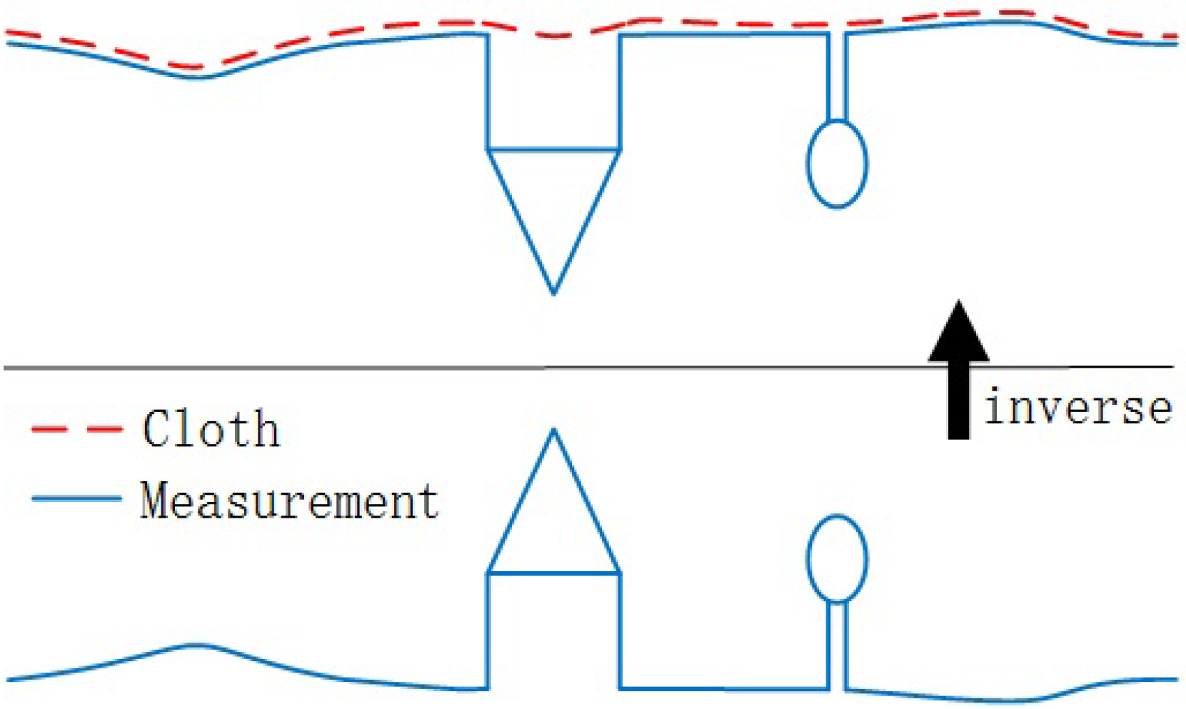
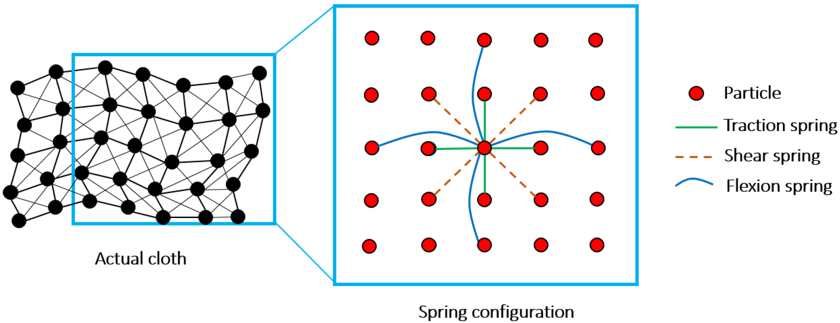
2.1. Fundamental of the Cloth Simulation
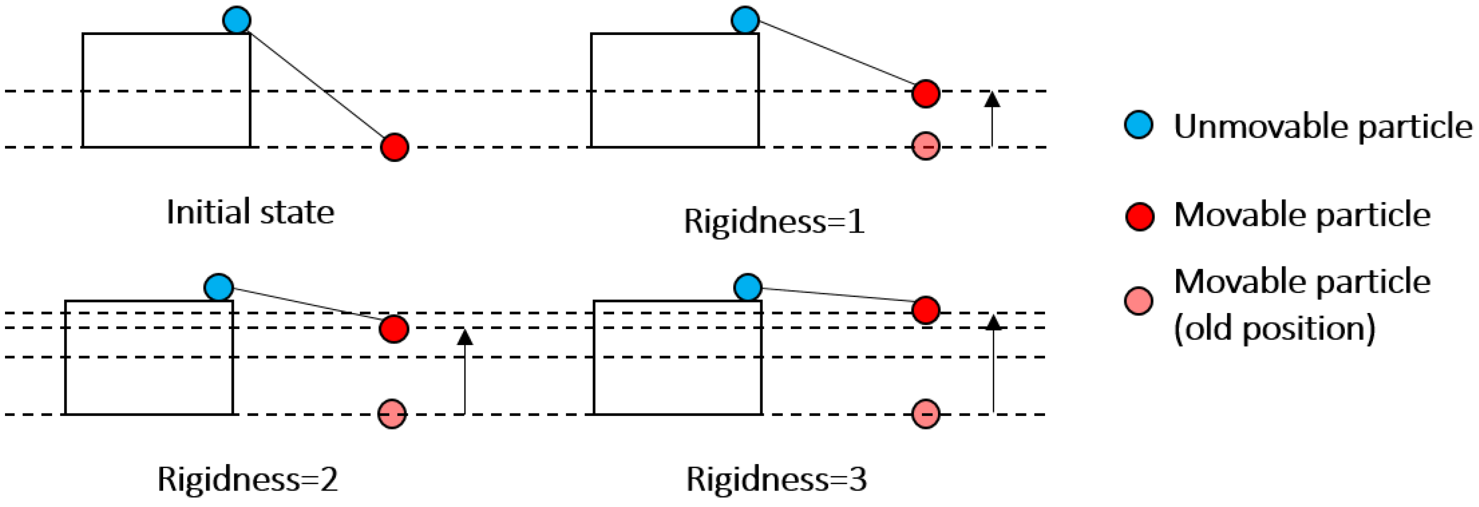
2.2. Modification of the Cloth Simulation
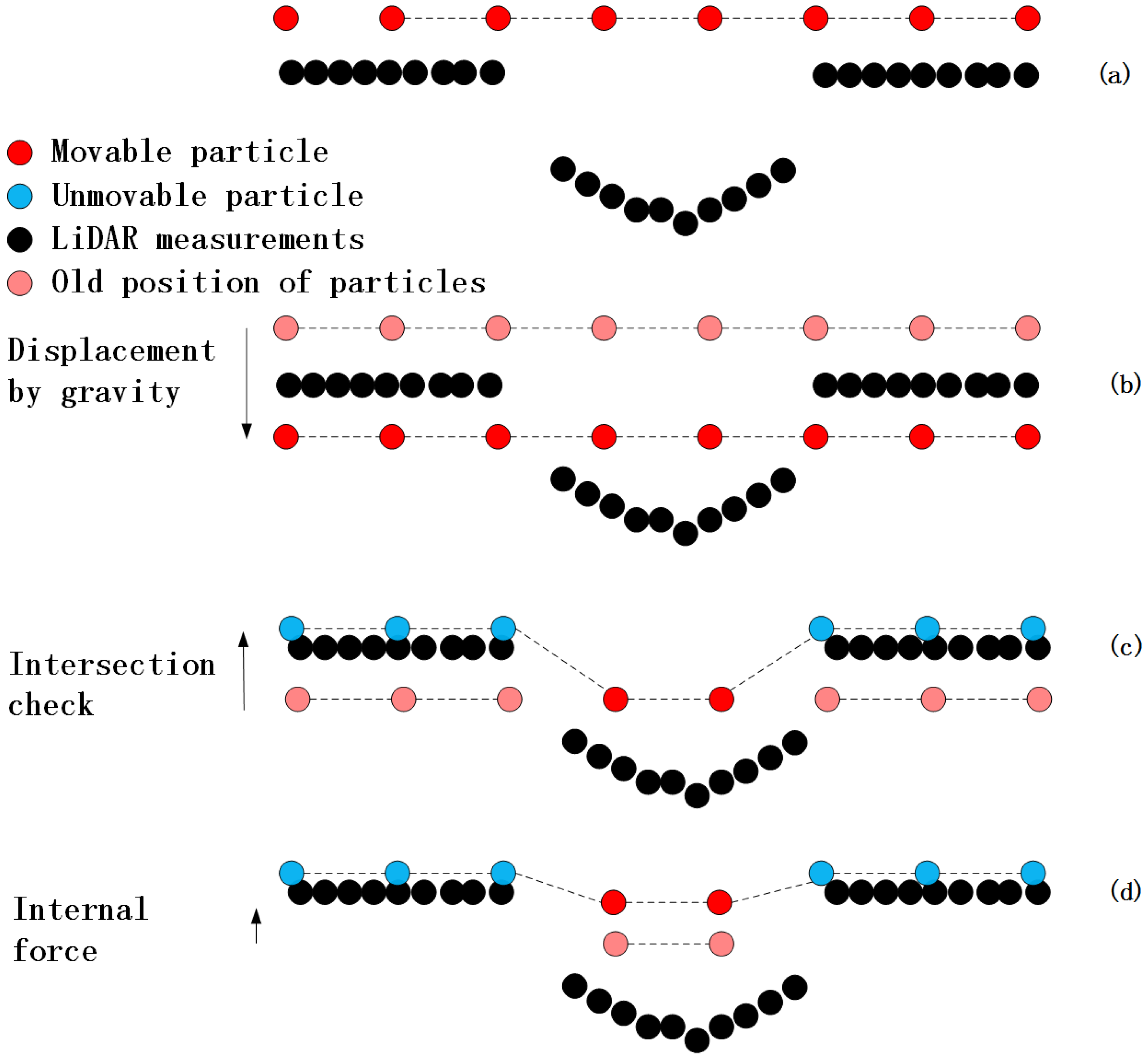
2.3. Implementation of CSF
- Automatic or manual outliers handling using some third party software (such as cloudcompare).
- Inverting the original LiDAR point cloud.
- Initiating cloth grid. Determining number of particles according to the user defined grid resolution (GR). The initial position of cloth is usually set above the highest point.
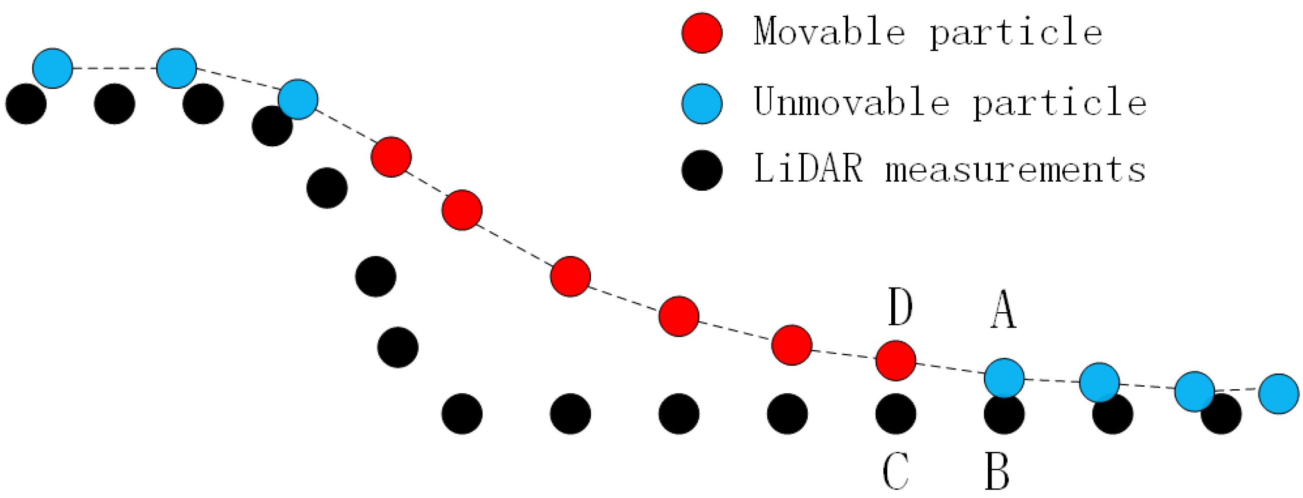
- Projecting all the LiDAR points and grid particles to a horizontal plane and finding the CP for each grid particle in this plane. Then recording the IHV.
- For each grid particle, calculating the position affected by gravity if this particle is movable, and comparing the height of this cloth particle with IHV. If the height of particle is equal to or less than IHV, then this particle is placed at the height of IHV and is set as “unmovable”.
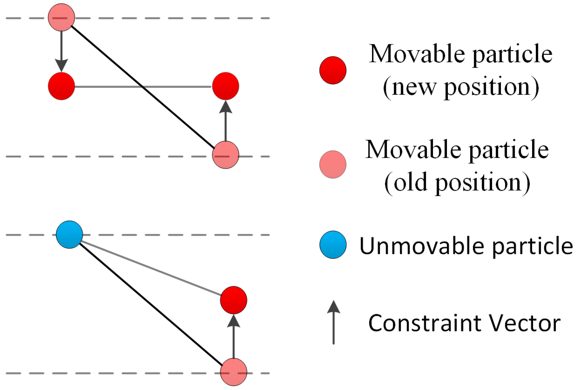
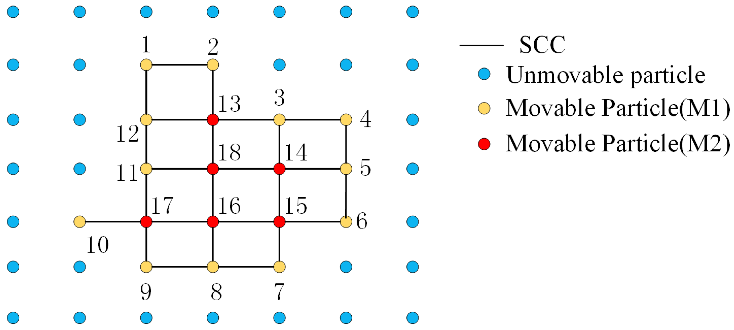
- For each grid particle, calculating the displacement of each particle affected by internal forces.
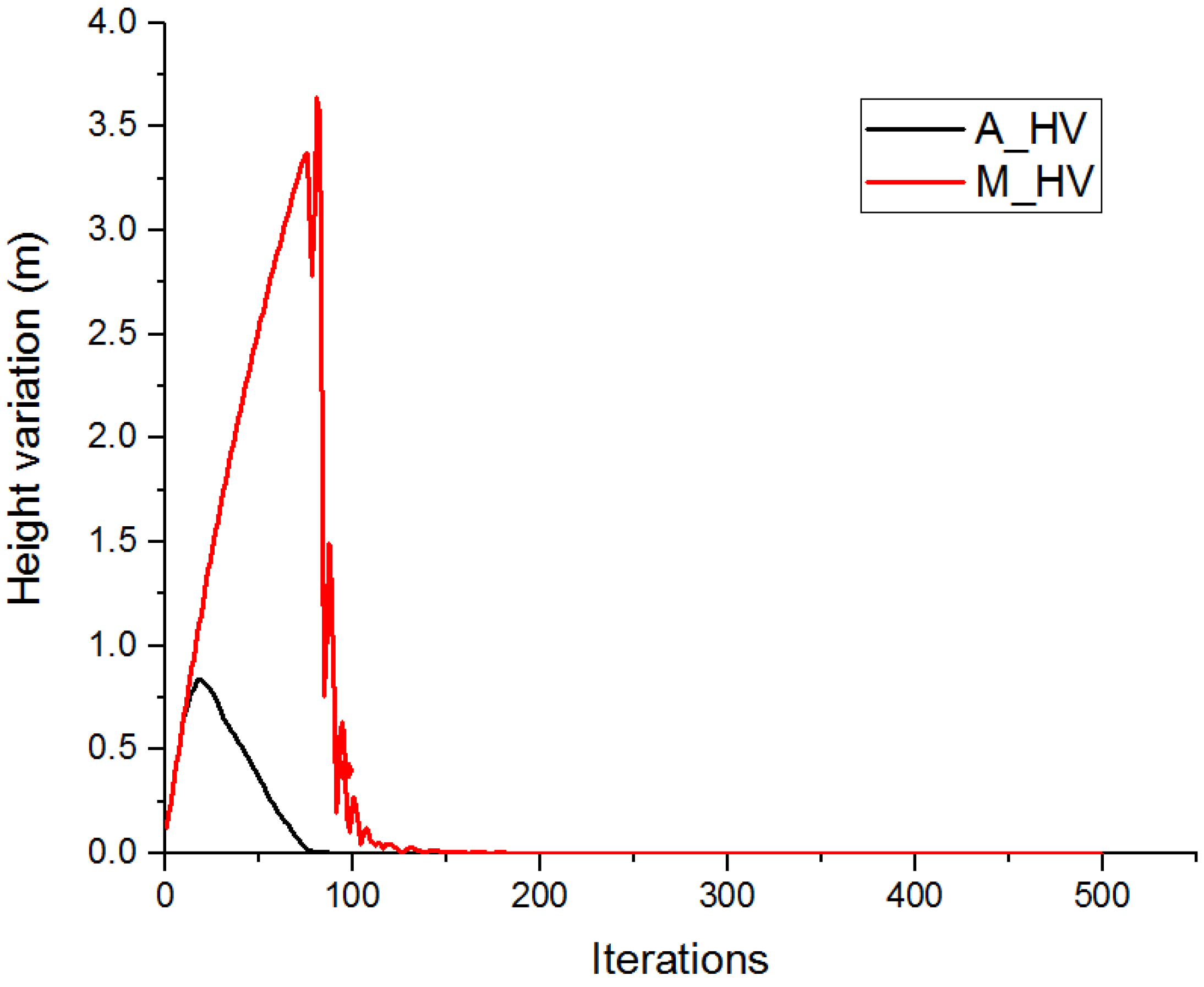
- Repeating (5)–(6). The simulation process will terminate when the maximum height variation (M_HV) of all particles is small enough or when it exceeds the maximum iteration number which is specified by the user.
- Computing the cloud to cloud distance between the grid particles and LiDAR point cloud.
- Differentiating ground from non-ground points. For each LiDAR points, if the distance to the simulated particles is smaller than , this point is classified as BE, otherwise it is classified as OBJ.
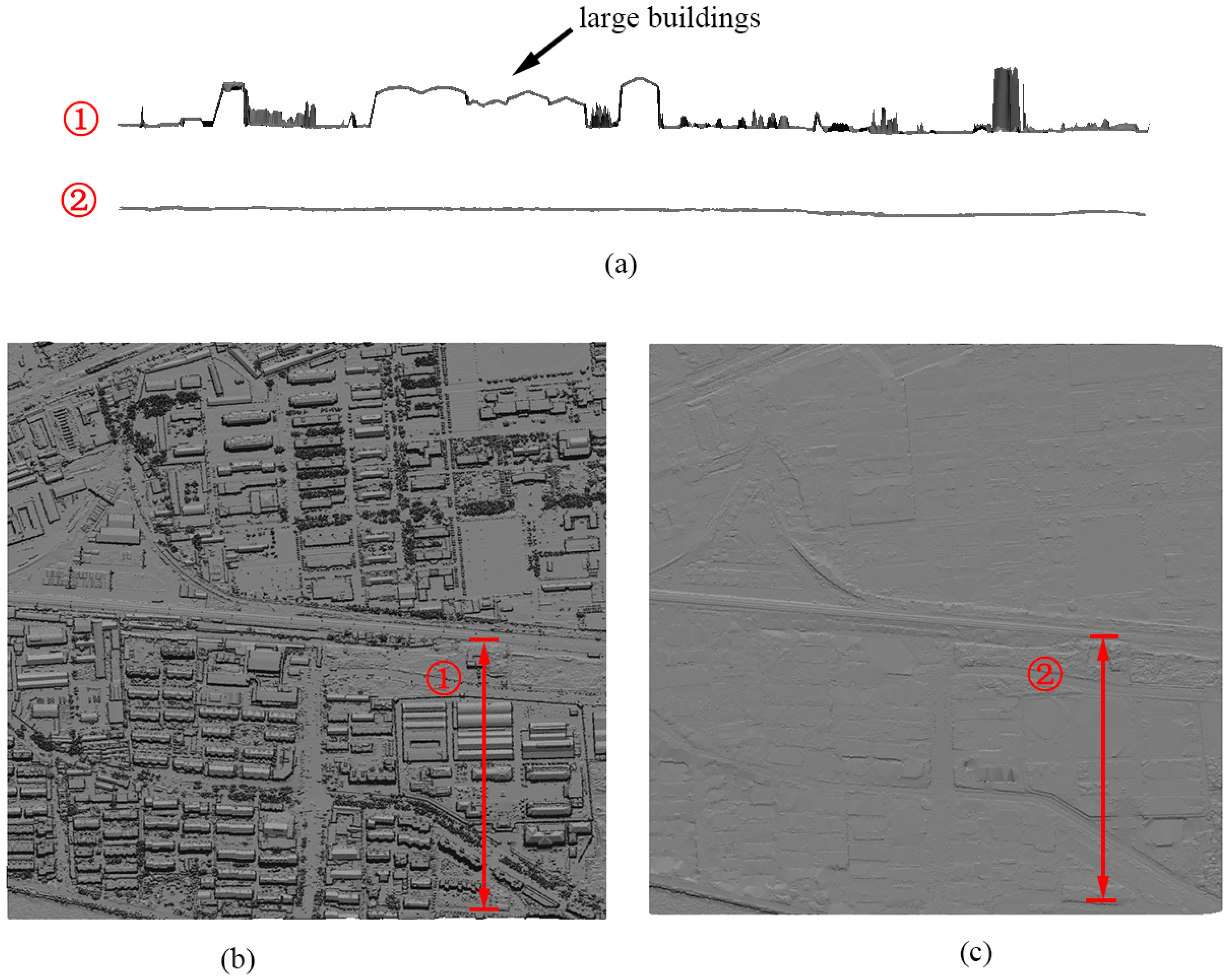
2.4. Post-Processing
2.5. Parameters
3. Experiment and Results
3.1. Validation of the Filtering
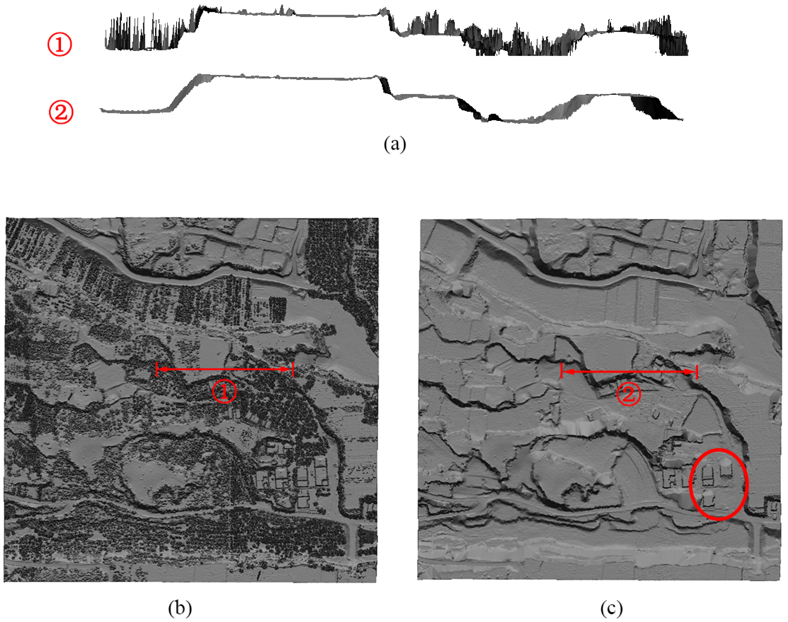
3.2. Testing with Dense Point Cloud
4. Discussion
4.1. Accuracy
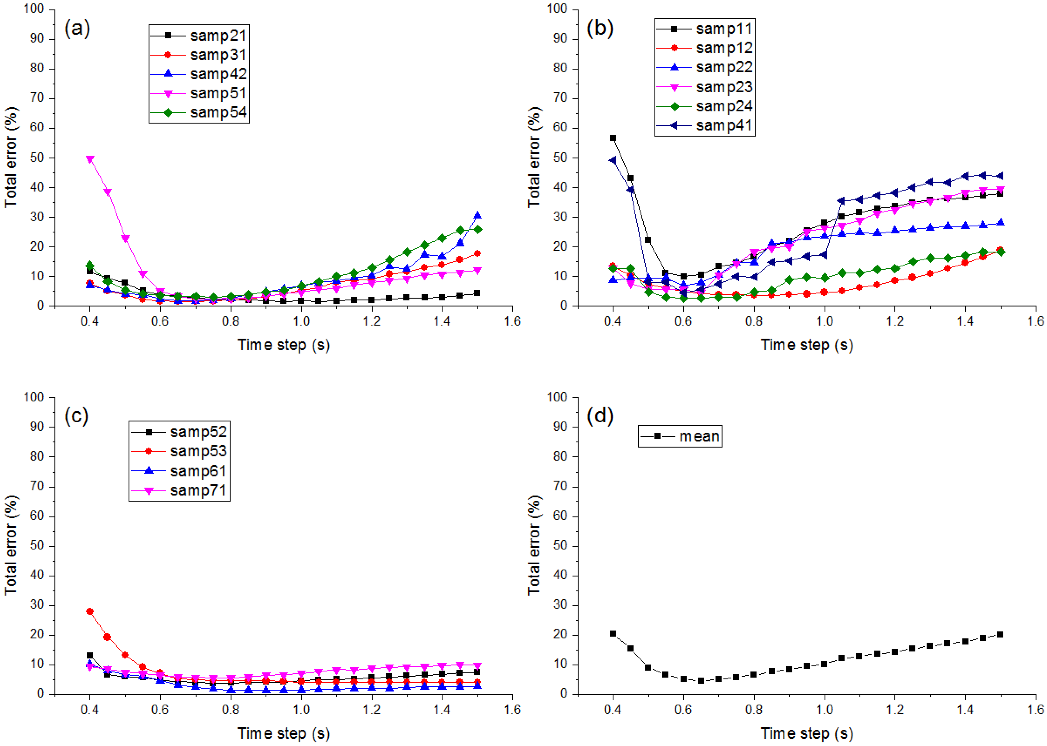
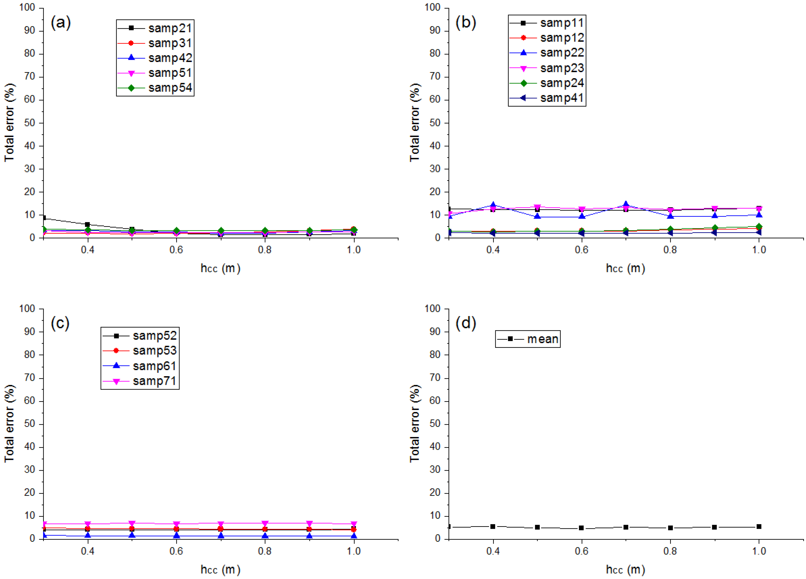
4.2. Parameter Setting
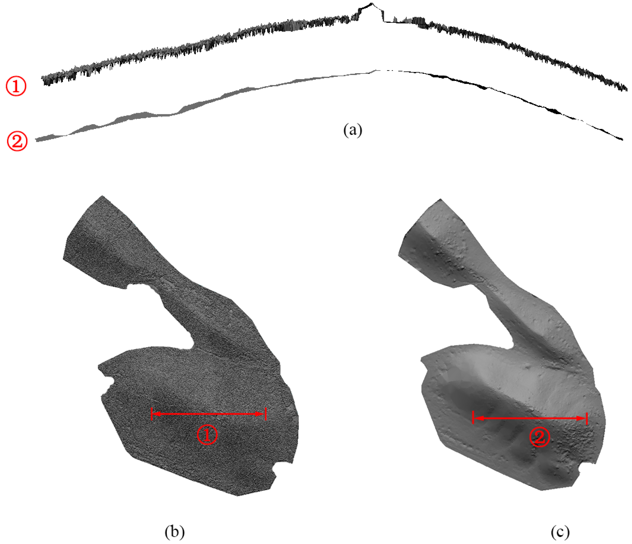
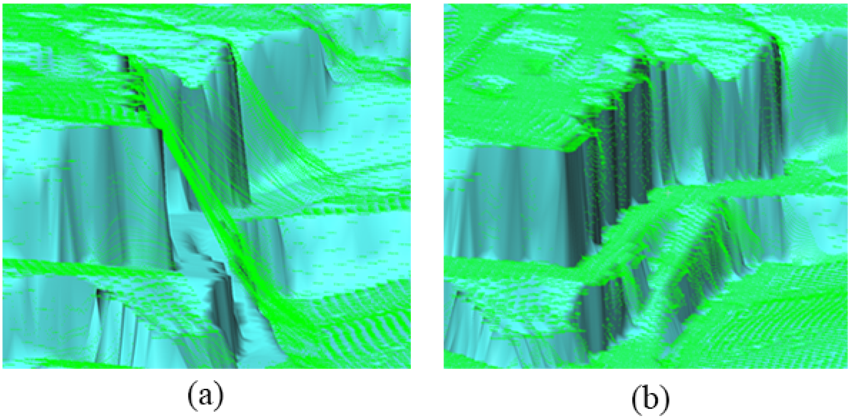
4.3. Steep Slopes
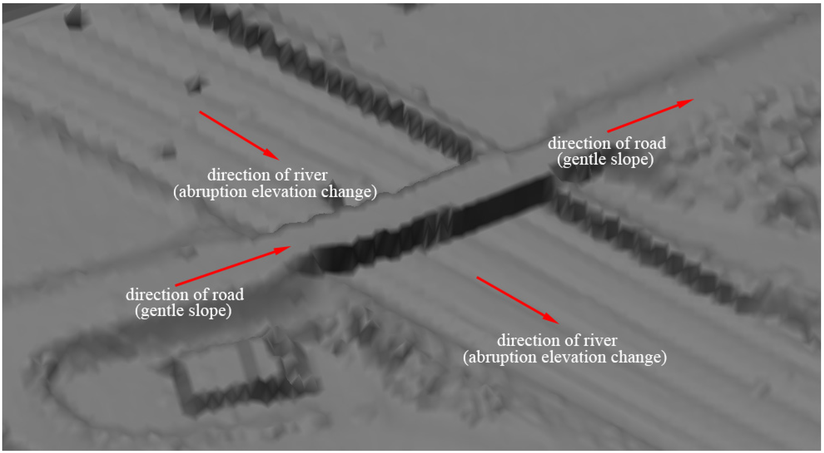
4.4. Bridge
4.5. Outlier Processing
5. Conclusions
Acknowledgments
Author Contributions
Conflicts of Interest
References
- Kobler, A.; Pfeifer, N.; Ogrinc, P.; Todorovski, L.; Oštir, K.; Džeroski, S. Repetitive interpolation: A robust algorithm for DTM generation from Aerial Laser Scanner Data in forested terrain. Remote Sens. Environ. 2007, 108, 9–23. [Google Scholar] [CrossRef]
- Vosselman, G. Slope based filtering of laser altimetry data. Int. Arch. Photogramm. Remote Sens. 2000, 33, 935–942. [Google Scholar]
- Shan, J.; Aparajithan, S. Urban DEM generation from raw lidar data. Photogramm. Eng. Remote Sens. 2005, 71, 217–226. [Google Scholar] [CrossRef]
- Meng, X.; Wang, L.; Silván-Cárdenas, J.L.; Currit, N. A multi-directional ground filtering algorithm for airborne LIDAR. ISPRS J. Photogramm. Remote Sens. 2009, 64, 117–124. [Google Scholar] [CrossRef]
- Sithole, G. Filtering of laser altimetry data using a slope adaptive filter. Int. Arch. Photogramm. Remote Sens. Spat. Inf. Sci. 2001, 34, 203–210. [Google Scholar]
- Susaki, J. Adaptive slope filtering of airborne LiDAR data in urban areas for digital terrain model (DTM) generation. Remote Sens. 2012, 4, 1804–1819. [Google Scholar] [CrossRef] [Green Version]
- Wang, C.K.; Tseng, Y.H. Dem generation from airborne LiDAR data by an adaptive dual-directional slope filter. In Proceedings of the ISPRS Commission VII Mid-Term Symposium 100 Years ISPRS—Advancing Remote Sensing Science, Vienna, Austria, 5–7 July 2010.
- Liu, X. Airborne LiDAR for DEM generation: Some critical issues. Progress Phys. Geogr. 2008, 32, 31–49. [Google Scholar]
- Sithole, G.; Vosselman, G. Filtering of airborne laser scanner data based on segmented point clouds. Int. Arch. Photogramm. Remote Sens. Spat. Inf. Sci. 2005, 36, W19. [Google Scholar]
- Zhang, K.; Chen, S.C.; Whitman, D.; Shyu, M.L.; Yan, J.; Zhang, C. A progressive morphological filter for removing nonground measurements from airborne LIDAR data. IEEE Trans. Geosci. Remote Sens. 2003, 41, 872–882. [Google Scholar] [CrossRef]
- Chen, Q.; Gong, P.; Baldocchi, D.; Xie, G. Filtering airborne laser scanning data with morphological methods. Photogramm. Eng. Remote Sens. 2007, 73, 175–185. [Google Scholar] [CrossRef]
- Li, Y. Filtering Airborne LIDAR Data by AN Improved Morphological Method Based on Multi-Gradient Analysis. ISPRS Int. Arch. Photogramm. Remote Sens. Spat. Inf. Sci. 2013, XL-1/W1, 191–194. [Google Scholar] [CrossRef]
- Li, Y.; Yong, B.; Wu, H.; An, R.; Xu, H. An Improved Top-Hat Filter with Sloped Brim for Extracting Ground Points from Airborne Lidar Point Clouds. Remote Sens. 2014, 6, 12885–12908. [Google Scholar] [CrossRef]
- Mongus, D.; Lukač, N.; Žalik, B. Ground and building extraction from LiDAR data based on differential morphological profiles and locally fitted surfaces. ISPRS J. Photogramm. Remote Sens. 2014, 93, 145–156. [Google Scholar] [CrossRef]
- Pingel, T.J.; Clarke, K.C.; McBride, W.A. An improved simple morphological filter for the terrain classification of airborne LIDAR data. ISPRS J. Photogramm. Remote Sens. 2013, 77, 21–30. [Google Scholar] [CrossRef]
- Mongus, D.; Žalik, B. Parameter-free ground filtering of LiDAR data for automatic DTM generation. ISPRS J. Photogramm. Remote Sens. 2012, 67, 1–12. [Google Scholar] [CrossRef]
- Axelsson, P. DEM generation from laser scanner data using adaptive TIN models. Int. Arch. Photogramm. Remote Sens. 2000, 33, 111–118. [Google Scholar]
- Zhang, J.; Lin, X. Filtering airborne LiDAR data by embedding smoothness-constrained segmentation in progressive TIN densification. ISPRS J. Photogramm. Remote Sens. 2013, 81, 44–59. [Google Scholar] [CrossRef]
- Kraus, K.; Pfeifer, N. Determination of terrain models in wooded areas with airborne laser scanner data. ISPRS J. Photogramm. Remote Sens. 1998, 53, 193–203. [Google Scholar] [CrossRef]
- Pfeifer, N.; Reiter, T.; Briese, C.; Rieger, W. Interpolation of high quality ground models from laser scanner data in forested areas. Int. Arch. Photogramm. Remote Sens. 1999, 32, 31–36. [Google Scholar]
- Chen, C.; Li, Y.; Li, W.; Dai, H. A multiresolution hierarchical classification algorithm for filtering airborne LiDAR data. ISPRS J. Photogramm. Remote Sens. 2013, 82, 1–9. [Google Scholar] [CrossRef]
- Su, W.; Sun, Z.; Zhong, R.; Huang, J.; Li, M.; Zhu, J.; Zhang, K.; Wu, H.; Zhu, D. A new hierarchical moving curve-fitting algorithm for filtering lidar data for automatic DTM generation. Int. J. Remote Sens. 2015, 36, 3616–3635. [Google Scholar] [CrossRef]
- Hui, Z.; Hu, Y.; Yevenyo, Y.; Yu, X. An Improved Morphological Algorithm for Filtering Airborne LiDAR Point Cloud Based on Multi-Level Kriging Interpolation. Remote Sens. 2016, 8, 35. [Google Scholar] [CrossRef]
- Elmqvist, M. Automatic Ground Modelling Using Laser Radar Data. Master’s Thesis, Linköping University, Linköping, Sweden, 2000. [Google Scholar]
- Guan, H.; Li, J.; Yu, Y.; Zhong, L.; Ji, Z. DEM generation from lidar data in wooded mountain areas by cross-section-plane analysis. Int. J. Remote Sens. 2014, 35, 927–948. [Google Scholar] [CrossRef]
- Weil, J. The synthesis of cloth objects. ACM Siggraph Comput. Graph. 1986, 20, 49–54. [Google Scholar] [CrossRef]
- Provot, X. Deformation Constraints in a Mass-Spring Model to Describe Rigid Cloth Behaviour; Graphics Interface; Canadian Information Processing Society: Mississauga, ON, Canada, 1995. [Google Scholar]
- Mosegaards Cloth Simulation Coding Tutorial. Available online: http://cg.alexandra.dk/?p=147 (accessed on 8 June 2016).
- Girardeau-Montaut, D. Cloud Compare-Open Source Project; OpenSource Project: Grenoble, France, 2011. [Google Scholar]
- Sithole, G.; Vosselman, G. Experimental comparison of filter algorithms for bare-Earth extraction from airborne laser scanning point clouds. ISPRS J. Photogramm. Remote Sens. 2004, 59, 85–101. [Google Scholar] [CrossRef]
- Cohen, J. A coefficient of agreement for nominal scales. Educ. Psychol. Measur. 1960, 20, 37–46. [Google Scholar] [CrossRef]
- Hu, H.; Ding, Y.; Zhu, Q.; Wu, B.; Lin, H.; Du, Z.; Zhang, Y.; Zhang, Y. An adaptive surface filter for airborne laser scanning point clouds by means of regularization and bending energy. ISPRS J. Photogramm. Remote Sens. 2014, 92, 98–111. [Google Scholar] [CrossRef]
- Terrasolid, Ltd. TerraScan User’s Guide; Terrasolid, Ltd.: Helsinki, Finland, 2010. [Google Scholar]
- Pfeifer, N.; Stadler, P.; Briese, C. Derivation of digital terrain models in the SCOP++ environment. In Proceedings of the OEEPE Workshop on Airborne Laserscanning and Interferometric SAR for Detailed Digital Terrain Models, Stockholm, Sweden, 1–3 March 2001; Volume 3612.
- CSF Software and Introduction. Available online: http://ramm.bnu.edu.cn/researchers/wumingzhang/english/default_contributions.htm (accessed on 8 June 2016).


| Environment | Site | Sample | Features |
|---|---|---|---|
| Urban | 1 | 11 | Mixture of vegetation and buildings on hillside |
| 12 | Buildings on hillside | ||
| 2 | 21 | Large buildings and bridge | |
| 22 | Irregularly shaped buildings | ||
| 23 | Large, irregularly shaped buildings | ||
| 24 | Steep slopes | ||
| 3 | 31 | Complex buildings | |
| 4 | 41 | Data gaps | |
| 42 | Railway station with trains | ||
| Rural | 5 | 51 | Mixture of vegetation and buildings on hillside |
| 52 | Buildings on hillside | ||
| 53 | Large buildings and bridge | ||
| 54 | Irregularly shaped buildings | ||
| 6 | 61 | Large, irregularly shaped buildings | |
| 7 | 71 | Steep slopes |
| Group | Feature | Parameters | Samples |
|---|---|---|---|
| I | Flat terrain or gentle slope, no steep slopes | RI = 3 ST = false | 21, 31, 42, 51, 54 |
| II | With steep or terraced slopes (e.g., river bank, ditch, terrace) | RI = 2 ST = true | 11, 12, 22, 23, 24, 41 |
| III | High and steep slopes (e.g., pit, cliff) | RI = 1 ST = true | 52, 53, 61, 71 |
| Samples | T.I(%) | T.II(%) | T.E.(%) | Kappa(%) |
|---|---|---|---|---|
| samp11 | 7.23 | 18.44 | 12.01 | 75.17 |
| samp12 | 1.15 | 4.9 | 2.97 | 94.04 |
| samp21 | 3.89 | 1.78 | 3.42 | 90.47 |
| samp22 | 1.29 | 25.9 | 8.94 | 77.72 |
| samp23 | 3.52 | 6.21 | 4.79 | 90.38 |
| samp24 | 1.03 | 7.73 | 2.87 | 92.68 |
| samp31 | 0.96 | 2.38 | 1.61 | 96.75 |
| samp41 | 1.48 | 8.78 | 5.14 | 89.73 |
| samp42 | 3.28 | 0.87 | 1.58 | 96.18 |
| samp51 | 2.67 | 4.57 | 3.08 | 91.13 |
| samp52 | 1.01 | 28.79 | 3.93 | 77.05 |
| samp53 | 3.85 | 37.08 | 5.2 | 46.86 |
| samp54 | 3.79 | 2.64 | 3.18 | 93.61 |
| samp61 | 0.87 | 18.94 | 1.49 | 78.1 |
| samp71 | 1.61 | 37.85 | 5.71 | 68.03 |
| Samples | Axelsson (1999) | Elmqvist (2000) | Pfeifer (2001) | Mongus (2012) | Li (2013) | Chen (2013) | Pingel (2013) | Zhang (2013) | Hu (2014) | Mongus (2014) | Hui (2016) | CSF |
|---|---|---|---|---|---|---|---|---|---|---|---|---|
| samp11 | 10.76 | 22.4 | 17.35 | 11.01 | 12.85 | 13.01 | 8.28 | 18.49 | 8.31 | 7.5 | 13.34 | 12.01 |
| samp12 | 3.25 | 8.18 | 4.5 | 5.17 | 3.74 | 3.38 | 2.92 | 5.92 | 2.58 | 2.55 | 3.5 | 2.97 |
| samp21 | 4.25 | 8.53 | 2.57 | 1.98 | 2.55 | 1.34 | 1.1 | 4.95 | 0.95 | 1.23 | 2.21 | 3.42 |
| samp22 | 3.63 | 8.93 | 6.71 | 6.56 | 4.06 | 4.67 | 3.35 | 14.18 | 3.23 | 2.83 | 5.41 | 8.94 |
| samp23 | 4.00 | 12.28 | 8.22 | 5.83 | 6.16 | 5.24 | 4.61 | 12.06 | 4.42 | 4.34 | 5.11 | 4.79 |
| samp24 | 4.42 | 13.83 | 8.64 | 7.98 | 5.67 | 6.29 | 3.52 | 20.26 | 3.80 | 3.58 | 7.47 | 2.87 |
| samp31 | 4.78 | 5.34 | 1.8 | 3.34 | 2.47 | 1.11 | 0.91 | 2.32 | 0.90 | 0.97 | 1.33 | 1.61 |
| samp41 | 13.91 | 8.76 | 10.75 | 3.71 | 6.71 | 5.58 | 5.91 | 20.44 | 5.91 | 3.18 | 10.6 | 5.14 |
| samp42 | 1.62 | 3.68 | 2.64 | 5.72 | 3.06 | 1.72 | 1.48 | 3.94 | 0.73 | 1.35 | 1.92 | 1.58 |
| samp51 | 2.72 | 21.31 | 3.71 | 2.59 | 3.92 | 1.64 | 1.43 | 5.31 | 2.04 | 2.73 | 4.88 | 3.08 |
| samp52 | 3.07 | 57.95 | 19.64 | 7.11 | 15.43 | 4.18 | 3.82 | 12.98 | 2.52 | 3.11 | 6.56 | 3.93 |
| samp53 | 8.91 | 48.45 | 12.6 | 8.52 | 11.71 | 7.29 | 2.43 | 5.58 | 2.74 | 2.19 | 7.47 | 5.2 |
| samp54 | 3.23 | 21.26 | 5.47 | 6.73 | 3.93 | 3.09 | 2.27 | 6.4 | 2.35 | 2.16 | 4.16 | 3.18 |
| samp61 | 2.08 | 35.87 | 6.91 | 4.85 | 5.81 | 1.81 | 0.86 | 16.13 | 0.84 | 0.96 | 2.33 | 1.49 |
| samp71 | 1.63 | 34.22 | 8.85 | 3.14 | 4.58 | 1.33 | 1.65 | 10.44 | 1.50 | 2.49 | 3.73 | 5.71 |
| Avg. | 4.82 | 20.73 | 8.02 | 5.62 | 6.18 | 4.11 | 2.97 | 10.63 | 2.85 | 2.74 | 5.33 | 4.39 |
| Std. | 3.44 | 15.92 | 5.09 | 2.39 | 3.84 | 3.06 | 2.00 | 6.01 | 2.03 | 1.64 | 3.23 | 2.76 |
| Samples | Axelsson (1999) | Elmqvist (2000) | Pfeifer (2001) | Chen (2013) | Pingel (2013) | Hu (2014) | Hui (2016) | CSF |
|---|---|---|---|---|---|---|---|---|
| samp11 | 78.48 | 56.68 | 66.09 | 74.12 | 83.12 | 82.97 | 72.92 | 75.17 |
| samp12 | 93.51 | 83.66 | 91 | 93.23 | 94.15 | 94.83 | 93.00 | 94.04 |
| samp21 | 86.34 | 77.4 | 92.51 | 96.1 | 96.77 | 97.23 | 93.35 | 90.47 |
| samp22 | 91.33 | 80.3 | 84.68 | 89.03 | 92.21 | 92.04 | 87.58 | 77.72 |
| samp23 | 91.97 | 75.59 | 83.59 | 89.49 | 90.73 | 91.14 | 89.74 | 90.38 |
| samp24 | 88.5 | 54.13 | 78.43 | 84.53 | 91.13 | 90.39 | 81.93 | 92.68 |
| samp31 | 90.43 | 89.31 | 96.37 | 97.76 | 98.17 | 98.19 | 97.33 | 96.75 |
| samp41 | 72.21 | 82.46 | 78.51 | 88.83 | 88.18 | 88.18 | 78.78 | 89.73 |
| samp42 | 96.15 | 90.86 | 93.67 | 95.81 | 96.48 | 98.25 | 95.38 | 96.18 |
| samp51 | 91.68 | 52.74 | 89.61 | 95.17 | 95.76 | 93.9 | 85.06 | 91.13 |
| samp52 | 83.63 | 9.36 | 41.02 | 78.91 | 81.04 | 86.24 | 69.51 | 77.05 |
| samp53 | 39.13 | 7.05 | 30.83 | 46.69 | 68.12 | 66.43 | 41.84 | 46.86 |
| samp54 | 93.52 | 55.88 | 88.93 | 93.9 | 95.44 | 95.28 | 91.63 | 93.61 |
| samp61 | 74.52 | 10.31 | 47.09 | 77.36 | 87.22 | 86.76 | 67.82 | 78.1 |
| samp71 | 91.44 | 26.26 | 75.27 | 93.19 | 91.81 | 92.59 | 79.86 | 68.03 |
| Avg. | 84.19 | 56.8 | 75.84 | 86.27 | 90.02 | 90.29 | 81.72 | 83.86 |
| Std. | 13.9 | 29.18 | 19.87 | 12.72 | 7.58 | 7.74 | 13.95 | 13.12 |
| Dataset | Type | Point Number | Scope | Features |
|---|---|---|---|---|
| 1 | Urban | 1559933 | 1 km × 1 km | Flat terrain, large and dense buildings, high vegetation coverage |
| 2 | Urban | 1522256 | 1 km × 1 km | Flat terrain with dense bungalow areas |
| 3 | Rural | 2093506 | 2 km × 1 km | dense vegetation coverage |
| 4 | Rural | 1418228 | 0.5 km × 0.5 km | Large number of steep slopes |
| Dataset | T.I(%) | T.II(%) | T.E.(%) |
|---|---|---|---|
| 1 | 0.72 | 13.36 | 6.84 |
| 2 | 5.29 | 9.29 | 7.84 |
| 3 | 36.09 | 1.84 | 5.49 |
| 4 | 8.57 | 22.61 | 14.09 |
© 2016 by the authors; licensee MDPI, Basel, Switzerland. This article is an open access article distributed under the terms and conditions of the Creative Commons Attribution (CC-BY) license (http://creativecommons.org/licenses/by/4.0/).
Share and Cite
Zhang, W.; Qi, J.; Wan, P.; Wang, H.; Xie, D.; Wang, X.; Yan, G. An Easy-to-Use Airborne LiDAR Data Filtering Method Based on Cloth Simulation. Remote Sens. 2016, 8, 501. https://0-doi-org.brum.beds.ac.uk/10.3390/rs8060501
Zhang W, Qi J, Wan P, Wang H, Xie D, Wang X, Yan G. An Easy-to-Use Airborne LiDAR Data Filtering Method Based on Cloth Simulation. Remote Sensing. 2016; 8(6):501. https://0-doi-org.brum.beds.ac.uk/10.3390/rs8060501
Chicago/Turabian StyleZhang, Wuming, Jianbo Qi, Peng Wan, Hongtao Wang, Donghui Xie, Xiaoyan Wang, and Guangjian Yan. 2016. "An Easy-to-Use Airborne LiDAR Data Filtering Method Based on Cloth Simulation" Remote Sensing 8, no. 6: 501. https://0-doi-org.brum.beds.ac.uk/10.3390/rs8060501