Early Detection of Summer Crops Using High Spatial Resolution Optical Image Time Series

Abstract

In the context of climate change, agricultural managers have the imperative to combine sufficient productivity with durability of the resources. Many studies have shown the interest of recent satellite missions as suitable tools for agricultural surveys. Nevertheless, they are not predictive methods. A system able to detect summer crops as early as possible is important in order to obtain valuable information for a better water management strategy. The detection of summer crops before the beginning of the irrigation period is therefore our objective. The study area is located near Toulouse (southwestern France), and is a region of mixed farming with a wide variety of irrigated and non-irrigated crops. Using the reference data for the years concerned, a set of fixed thresholds are applied to a vegetation index (the Normalized Difference Vegetation Index, NDVI) for each agricultural season of multi-spectral satellite optical imagery acquired at decametric spatial resolutions from 2006 to 2013. The performance (i.e., accuracy) is contrasted according to the agricultural practices, the development states of the different crops and the number of acquisition dates (one to three in the results presented here). The detection of summer crops reaches 64% to 88% with a single date, 80% to 88% with two dates and 90% to 99% with three dates. The robustness of this method is tested for several years (showing an impact of meteorological conditions on the actual choice of images), several sensors and several resolutions.

1. Introduction

In a context of global climate change, corroborated by a temperature increase [1], a change in the precipitation regime [2] and an increase in world population, farming techniques need to be able to achieve sufficiently high yields. Agriculture has to satisfy food supply needs, while minimizing the use of natural resources and its environmental impact [3]. For example, farming is the main consumer of limited water resources [4]. Agricultural practices are therefore a major concern because of their environmental impact, the amount of water they use and the quantity of food they are able to supply. Since irrigated croplands provide a large fraction of the world agricultural production, ensuring a balance between the needs for irrigation and the resources available is a crucial objective. In this context, land use and land cover changes over time, which mainly result from anthropic and natural factors, are key parameters. Farming practices are organized within the landscape depending on different internal and external constraints (climate, soil, size of the plots, water availability, social and cultural constraints, etc.). The choice and the implementation of these practices are guided by local factors (production methods, work management at farm scale), local policies, and national and international regulations [5].

As specified by McNairn et al. [6] most of the regional and international initiatives for agricultural management have so far been based on information coming from in situ data. Meanwhile, satellite imagery, offering observations in a wide range of wavelengths, with large spatial and frequent temporal observation capabilities, has been widely used for land use mapping [7,8], crop monitoring [9,10,11,12], identification of agricultural practices [13,14] and estimation of yield and crop parameters [15,16,17,18,19]. Until now, crop map production with identification of summer crops (i.e., corn, sunflower, sorghum, soybean, hemp), with accurate information about their location using multi-temporal image classification, has been possible only at the end of the crop season [20,21]. This late detection is a problem for water resource management and earlier availability of this information during the spring, before the beginning of the irrigation period, would allow the implementation of better strategies at watershed scale. In this context, McNairn et al. [6] investigated the possibility of early-season monitoring for two agricultural classes (soybean and corn) using TerraSAR-X and Radarsat-2 time series. Additionally, the increasing availability of high spatial and temporal resolution imagery thanks to recent or upcoming systems (Landsat 8, Sentinel-2, Venµs), may provide land managers with information about crop status and crop area extents at the watershed and landscape scales. These new missions will give access to near-real-time images allowing operational crop management as well as early land-use detection [22,23,24,25].

Phenology is defined as the periodicity of key events in the life cycle of living species, their chronology and their relationship with weather and climate [26]. In the case of crops, an understanding of phenology is needed for irrigation planning, fertilizer management, yield forecasting and greenhouse gas studies [27,28,29]. The Normalized Difference Vegetation Index (NDVI), which is computed with the reflectances in the red and near-infrared spectral bands, allows active vegetation to be distinguished from other types of land cover [30,31]. Furthermore, a temporal analysis of the NDVI follows the evolution of crop phenology as well as land cover changes, to predict yield forecasts as recently presented in [32].

The goal of this work is to propose an accurate and easily reproducible method that allows early detection of summer crops, before the start of irrigation period, and discriminates them from other kinds of vegetated surfaces, either other crops or grasslands. The main difficulty of such a method lies in distinguishing grasslands from some crop types because of their similarity in phenology and, therefore, in NDVI evolution through time. In order to identify summer crops at their earliest stages of development, or even before they are sown, the method uses a decision tree. The paper is organized as follows: the first section (§2) presents the data used; (§3) the analysis of historical data (2006 to 2013) leading to the proposed approach; and finally, the results are presented (§4) using different approaches: a study of the chronological addition of dates and a summarized analysis of several years of data.

2. Materials

Between 2006 and 2013, annual measurement campaigns enabled the acquisition of satellite images and in situ observations, providing the basis for our study. We also used exogenous data (meteorological data, topographical land parcel information system). The characteristics of all data needed for the study are presented in the sections below.

2.1. The Study Site

Agricultural plots throughout France are very diverse in terms of size and shape despite agricultural reparceling, which began in 1941 [33], and the study site is part of this heritage. It is located in the southwest of France (Figure 1), a region with a typical temperate climate. The average daily air temperature ranges from a few degrees above freezing in winter to 22 °C in summer, according to the SAFRAN [34] 8 km resolution gridded data set over the 2007–2013 period). The annual rainfall usually amounts to 600 mm (ranging from 510 mm in 2011 to 767 mm in 2008). In this region of alluvial plains and hills, the steepest slopes are mainly found in the transition areas between low and high altitudes.

The site is oriented towards polyculture/livestock, and is composed of crops, forests, urban areas, grasslands and water bodies. Crops are divided into two categories: winter crops mainly represented by wheat, barley and rapeseed, and summer crops, both irrigated (corn and soybean) and non-irrigated (sunflower, sorghum and hemp). The NDVI time series of the two crop types and grasslands are shown Figure 2. The lines plotted correspond to the mean values computed over 7 consecutive years, which smooth the intra-class and inter-annual variability.

Winter crops such as wheat and barley emerge in autumn (November/December), present a latency phase in winter (January/February) and a new growth phase in spring. Harvest takes place in summer. Barley is sown at the same time as wheat, but generally matures earlier. A few late barley varieties emerge in spring, and are harvested at the end of the summer. Rapeseed has a long vegetation cycle (emergence in September, flowering in April/May and harvest in July). Despite a strong heterogeneity in its development during the growing season, rapeseed can fully cover the soil at the end of flowering [35,36].

Overall, the emergence of summer crops is spread over about 3 months between April and July, with a peak in late April. Ninety percent of summer crops emerge between late April and early June. Sunflower has a short vegetation cycle (lasting between 120 and 150 days), depending on the variety and on climatic conditions. Emergence occurs between April and June, harvest begins at the end of summer (September) and continues throughout autumn (November). The plots of sunflower are often heterogeneous in terms of vegetation development and density. The emergence of corn, soybean and sorghum begins at the end of April, with harvest ranging from October to November. About 85% of corn and soybean crops grown in the monitored area are irrigated. Hemp also emerges at the end of April, and the vegetation cover is high in May (about 90% three weeks after emergence). Flowering begins in June, and harvest takes place in September.

Finally, grasslands are composed of several plant species that do not have the same seasonal phenological behavior. Their actual phenological cycle depends on the species, the weather conditions, the soil type and the use (hayfields or grazed grasslands), explaining the large differences observed between the plots of grassland.

The period following the harvest of a crop is handled differently according to the individual farmers. Some of them plow and then leave the soil bare while waiting for the establishment of the next crop. Others carry out light tillage promoting regrowth and, thus, have vegetated ground. Others do nothing, letting nature take its course. Whatever the chosen solution, a change of soil state occurs before the next crop is planted (stubble disked, deeply plowed, tilled soil, prepared soil).

2.2. Satellite Images

The proposed approach was designed by analyzing multi-spectral Formosat-2 and Spot (4 and 5) images, regularly acquired during successive agricultural seasons from 2006 to 2013. The main characteristics of the satellite images are presented below.

The Taiwanese satellite Formosat-2 was launched in May 2004 on a sun-synchronous orbit. It produces optical images using push-broom sensors (in the visible and short-wave infrared domains) with high spatial resolution (8 m in multi-spectral and 2 m in panchromatic modes), with a constant viewing angle: 45° lateral and 45° forward-backward looking [37]. Each image covers an area of 24 × 24 km².

Spot 4 was launched in March 1998. It was finally deorbited, when the Take5 program [38] took place (from February to June 2013) to prepare further analyses of time series acquired by ESA’s Sentinel-2 mission. Spot 5 was launched in May 2002. Spot satellites are on a sun-synchronous orbit. They produce optical images using push-broom sensors (in the visible, and near and shortwave infrared domains) with high spatial resolution (20 m for Spot 4, 10 m for Spot 5 in multi-spectral mode and 0.60 m in panchromatic mode), with a variable viewing angle (except during the Take5 period). Each image covers an area of 60 × 60 km² and 60 × 220 km² for Take5.

These images are processed by CNES in the framework of the “Kalideos” program [39]. All the images are ortho-rectified using CNES ortho-rectification tools. Cloud detection and atmospheric correction are also applied, providing Top of Canopy images (TOC) [40]. The average location accuracy is about one pixel. All these satellites operate in the optical domain with red and near infrared spectral bands, which allows the NDVI to be computed.

From 2006 to 2013, 93 images were collected for the study area. Note that there were no images available throughout the winter and spring of 2008. For the proposed evaluation, three images were used per year. They had to be acquired between February and June, the precise dates depending on availability. For the years 2006–2013, during this month range, 45 satellite images were available (

Table 1. Monthly temporal distribution of the satellite images for the different years.

	January	February	March	April	May	June	July	August	September	October	November	December
2006	−	2	1	1	2	2	5	2	2	1	2	−
2007	−	1	−	1	1	1	1	2	2	1	−	−
2009	−	1	3	−	1	2	3	4	2	1	−	−
2010	2	1	2	3	2	2	5	3	4	1	−	−
2011	1	1	1	3	1	−	1	1	2	−	−	−
2012	−	1	1	−	1	1	−	−	−	−	−	−
2013	−	2	1	1	−	2	−	−	−	−	−	−

): 23 Formosat-2, 12 Spot 4, 4 Spot 5 and 6 Spot 4 Take5 (Figure 1).

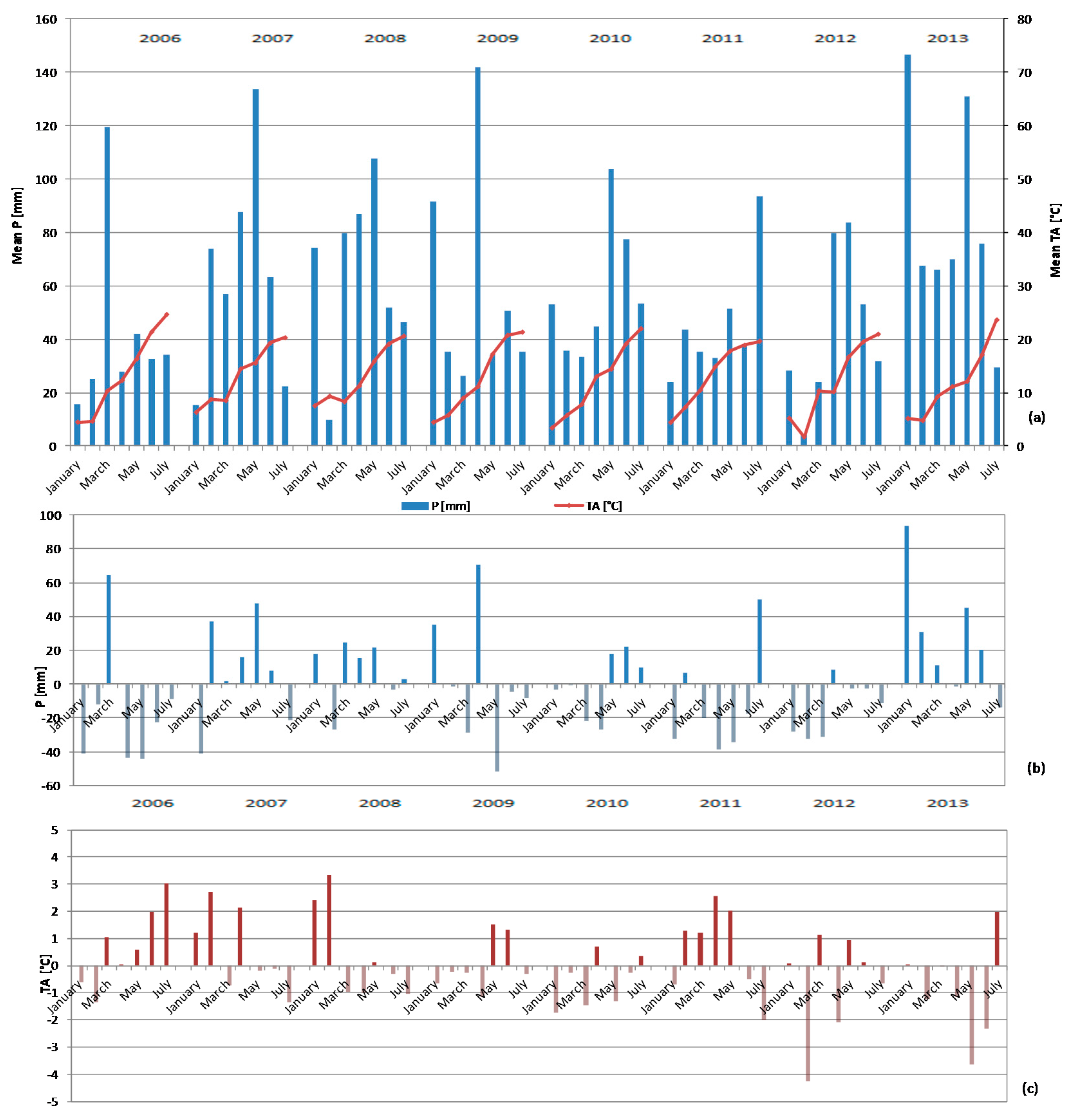
2.3. Meteorological Data

The phenological evolution depends on the sowing dates, which in turn depend on weather conditions. The SAFRAN database [34] was used in order to understand this relationship. SAFRAN meteorological data are provided on an 8 km grid and contain the air temperature at 2 m above the ground (TA), the solar irradiation (Rg) and precipitation (P) every 6 h.

Figure 3 shows the climatological changes on our study site for the first half of the years under study. Episodes of rain are recurrently observed in the spring.

These episodes of rain and/or cold spring are prejudicial for planting summer crops, since they should be sown in a “dry” and warm soil to ensure that they come up rapidly and grow steadily so as to be less exposed to external agents (birds, slugs, etc.). Three years, contrasting in terms of distribution of spring rainfall and sowing period for summer crops, and representative of the climate of our study area will be particularly highlighted in this study: 2007, 2009 and 2013.

In 2009, spring rain occurred mainly in April (142 mm) while in 2007 and 2013, it occurred in May, with 134 mm and 131 mm respectively. From January to June, the cumulated precipitations reached 431 mm in 2007, 380 mm in 2009 and 560 mm in 2013. The average of atmospheric temperature for May was 15.5 °C in 2007, 17.2 °C in 2009 but only 12 °C in 2013. The average through the first semester was 12.1 °C in 2007, 11.4 °C in 2009 and 9.9 °C in 2013. Therefore, spring may be regarded as having been average in 2007, rainy but warm in 2009 and rainy and cold in 2013.

2.4. Land Use Reference Data

2.4.1. Topographical Land-Parcel Information System

The French Services and Payment Agency has been providing a topographical land-parcel information system containing information on the crop types of agricultural plots since 2007. It is known as the Registre Parcellaire Graphique (RPG) and is used for the management of European agricultural subsidies. The inter-annual RPG changes in the contours of plots are minor (ranging from 1.2% between agricultural seasons 2010/2011 to 4.8% for 2007/2008). Since 2010, the location of agricultural areas has remained stable, with annual changes lower than 1.5%. This allows us to use the RPG data base of the previous year to mask out areas that do not correspond to grasslands and croplands for the analysis.

2.4.2. In Situ Data

Over 500 plots were monitored every year from 2006 to 2013 (Figure 1). The sampled plots were characterized by a wide variety of shapes (square, rectangular, circular or triangular) and sizes ranging from 0.14 to 24.6 ha. The information collected was: crop type, surface state between main crops (defined as inter-crop state), soil tillage before sowing and emergence date. These data were used both for the validation of the summer crop detection, and for the interpretation of the results, mainly by taking the soil work before sowing into account.

3. Methodology

The proposed method is based on the exploitation of multi-temporal satellite imagery acquired before or during the emergence of summer crops (Figure 2). The approach uses the Normalized Difference Vegetation Index (NDVI) derived from the red and near-infrared spectral bands. The main advantage of using such a normalized index is that it can cope with slight differences between sensors (i.e., viewing angles and spatial resolutions [41]) and it is sensitive to the fraction of ground covered by the vegetation.

To design a robust method, several years of data were analyzed (2006–2013). This made it possible to implement an approach that could withstand differences in climate and imagery availability. The method was based on decision tree methodology, applying thresholds on NDVI, using 1 to 3 optical images. The analysis of crop phenology and successive surface states (§3.1) enabled thresholds and decision rules to be determined (§3.2) and then applied to the selected images (§3.3).

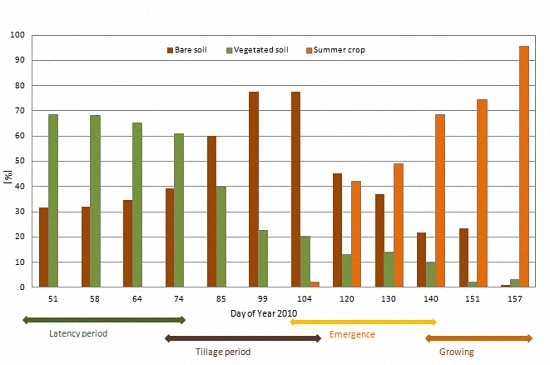
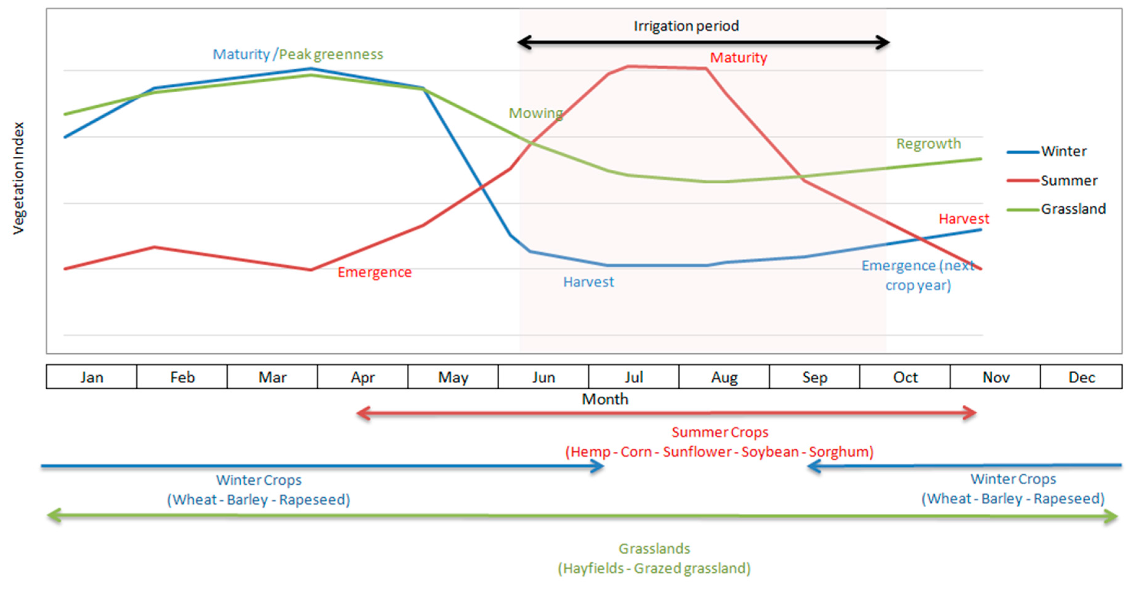
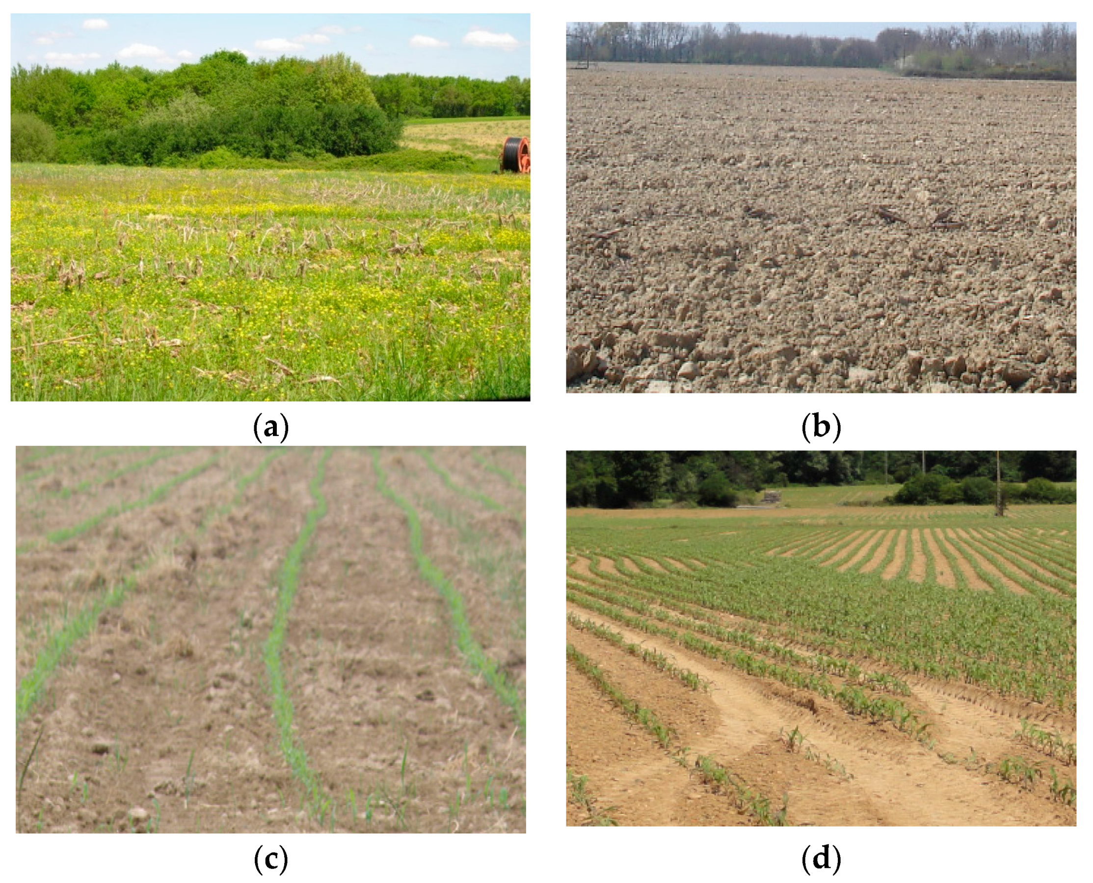
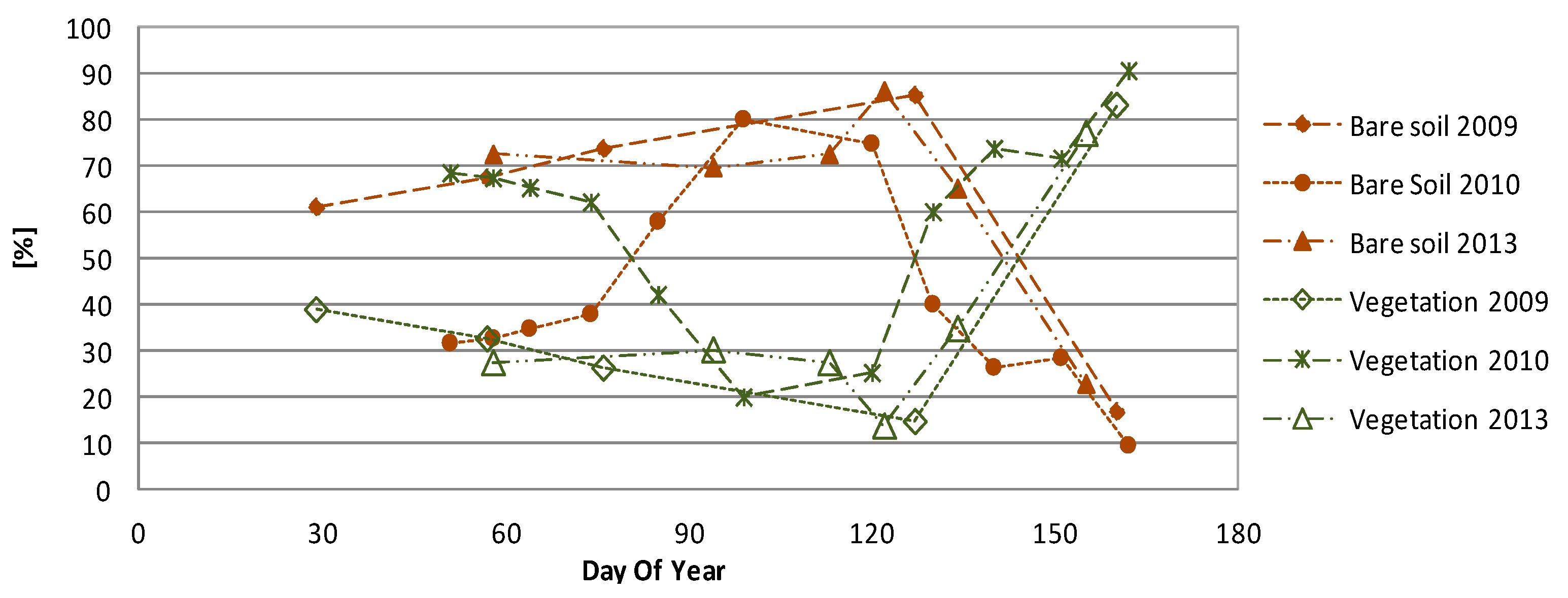
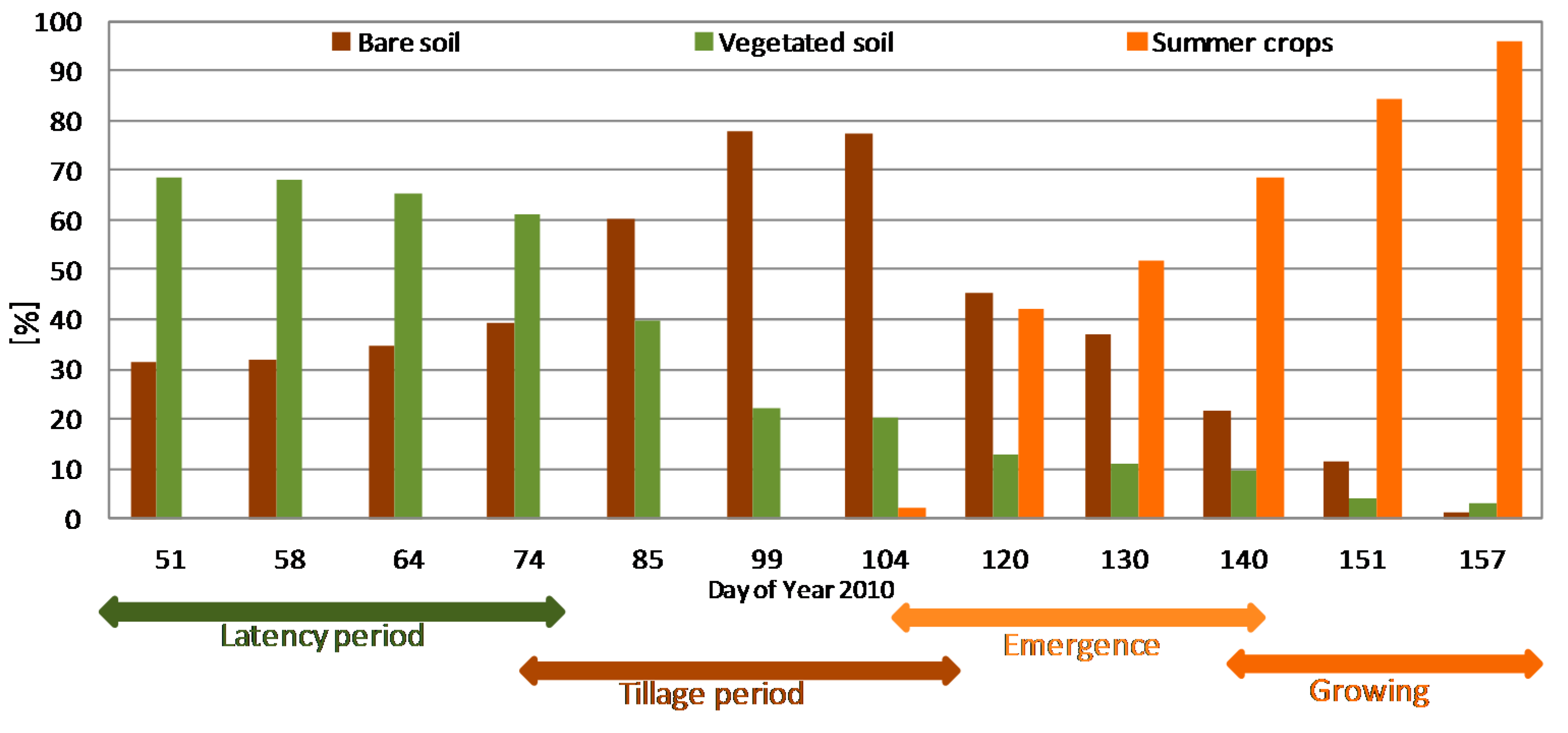
3.1. Study of Crop Phenology and Surface State

Using the imagery available for the whole set of years, the mean NDVI profiles were computed for each crop. To illustrate the annual climatic differences, these profiles are designed and presented for all the available years. They are a proxy for the phenology of each crop, which identifies the best periods for the discrimination between summer crops, winter crops and grasslands.

The agricultural calendar is based on the constraints imposed by crop seasonality, climatic events, and also by farmers’ choices and constraints. Some decisions are taken at farm scale, depending on the total amount of work that has to be done and the human resources and machinery available. Despite these local and varied constraints, we observed that the mean NDVI of winter crops (wheat, rapeseed and barley) and grasslands were always higher than 0.5 during the growing phase, between April and June (Day 90 to Day 150, in Figure 4), whatever the year, the climatic conditions or the soil type. On the other hand, summer crops (corn, sunflower, sorghum, soybean and hemp) had not emerged yet and their mean NDVI was lower than 0.4 (Figure 4). A stability of the crops in terms of heterogeneity was also observed.

For instance, in 2006, between 15 February (Day 45, before the beginning of summer crop sowing) and 15 June (Day 166, after the end of sowing), the average NDVI per crop field for summer crops ranged from 0.13 (characteristic of a bare soil) to 0.5 (characteristic of dense vegetation). This last level of NDVI can be related to two surface states: regrowth of the previous year’s crop (Figure 5a) with or without self-sown vegetation, or a growing phase of the crop (Figure 5c,d). After harvest, farmers choose among several possibilities: carrying out deep soil work, letting vegetation regrow and destroying it just before the next sowing, or sowing directly (without any preliminary preparation). In any case, for all the years studied, it was observed that the change from vegetation cover (Figure 5a) to bare soil (Figure 5b) exhibited a phase where crop NDVI was lower than or equal to 0.3. Therefore, a bare soil phase, which depends on several factors, preceded the sowing of summer crops (between April and June).

Figure 6 shows the evolution of surface states for the years 2009, 2010 and 2013. Among the 500 plots monitored, the percentage of bare soil increased during the winter period and reached its maximum between 1 April and 15 May (Days 90 to 135) for 85% of summer crop fields. For all the years studied, summer crops emerged around 15 June (Day 166).

The optimal period for the detection of potential summer crops is therefore between the beginning of April and the beginning of June (Days 90 to 150) (Figure 4). Therefore, this period of bare soil or of weak revegetation is suitable for our NDVI thresholding based approach (Figure 6).

To determine precise NDVI values that allowed summer crop plots to be differentiated from other surface states, analyses were performed on land use data collected synchronously with satellite images. For instance, on 17 March 2009, the ground data contained 50 plots of bare soil and 20 vegetated plots before planting. The NDVI of bare soil plots ranged from 0.12 to 0.41 (mean NDVI of 0.26), the maximal values being associated with plots in which weeds were growing (covering less than 30% of the total area). For vegetated and emerged plots, NDVI ranged from 0.14 to 0.51 (mean NDVI of 0.33).

Similar analyses were performed on the data collected between Days 46 and 123, and showed that values of NDVI ranged from 0.2 to 0.4, on plots dedicated to the cultivation of summer crops. Finally, the analyses of the surface states were summarized as the following values: 0.2 for totally bare soil (Figure 5b), 0.3 for very poorly vegetated ground (Figure 5c), 0.35 for vegetated or weakly emerged soil (2–4 leaves over at least 50% of the plot) (Figure 5d), 0.4 for vegetated soil or effective emergence (Figure 5a). These values and their temporal succession are used to isolate summer crops in the decision tree in the section below, minimizing confusion with winter crops and grasslands.

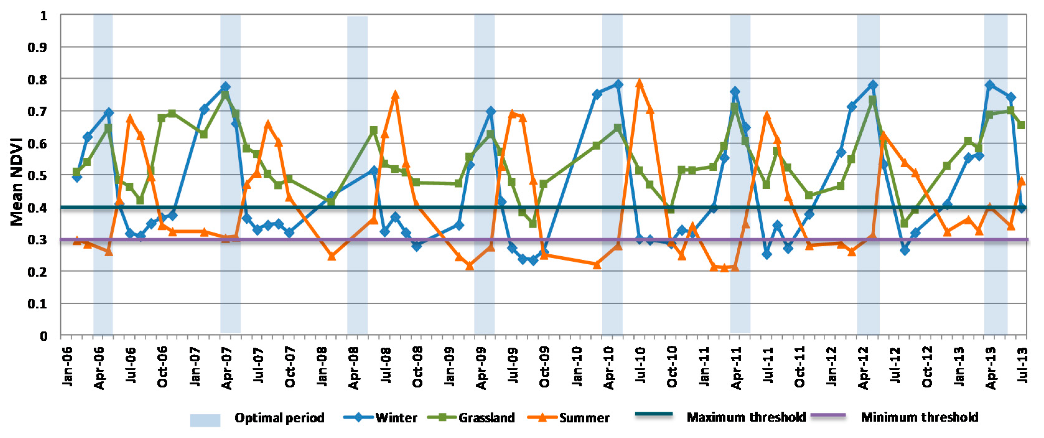
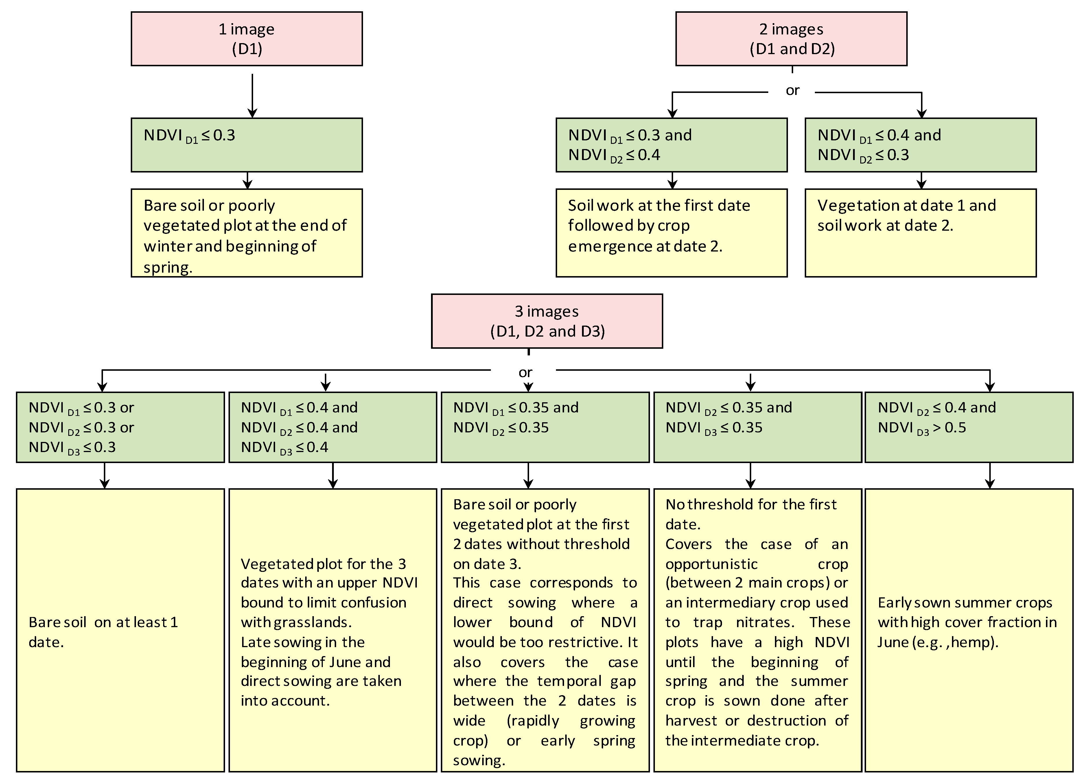
3.2. NDVI Thresholding

The proposed method for the detection of summer crops is based on a decision tree using thresholds on NDVI values (with values provided by the preliminary analysis). It uses 1 to 3 dates, which are added chronologically.

First of all, the RPG is used as a mask so that only the agricultural areas (main crops and grasslands) are included. Multi-temporal NDVI thresholding is then used in order to distinguish summer crop pixels from the other 2 classes (winter crops and grasslands). The threshold values are chosen according to the analysis presented in Section 3.1 and are available in Figure 7.

The use of a single date (D1) allows bare soils to be detected. The combined use of 2 dates (D1 and D2) identifies bare soils and vegetated plots. The joint use of 3 dates (D1, D2 and D3) detects summer crops, taking temporal shifts in soil working and sowing into account, and also differences in crop growing speeds. The soil is either vegetated or bare and the crop is either emerging or has a high cover fraction. In this way, the four surface states can be distinguished.

3.3. Selection of the Optimal Temporal Window

Although the optimal period for the detection of summer crops using NDVI is from April to June (Days 90 to 150), the image availability may vary (depending mainly on the cloud cover).

To evaluate the robustness of the proposed approach, a temporal window going from February to June was used. It covered the growing stages of winter crops until the beginning of the growing period of summer crops and their irrigation (Figure 2).

For each year, the three images that were the closest to this period were chosen. If no image was available during this period, the temporal window was widened. In an operational context, with the upcoming multi-temporal missions, one image should be available per month. If more than 3 images are available in the period, a gap of one month between successive acquisitions will be chosen in order to cover different possible surface states.

Figure 8 shows that the surface states change progressively. Tillage events before sowing explain the increase of bare soil during the months of March and April, which is gradually masked by the development of crops. A repetitiveness of one month between satellite images seems both sufficient to observe the various surface states and necessary so that the plots present enough changes (e.g., a time lag of one month is observed between sowing and emergence). Following these heuristics, the selection of dates for each year is shown in

Table 2. Description of the image dates used for each year.

Years	2006 Formosat-2	2007 Formosat-2	2009 Formosat-2	2010 Formosat-2	2010 Spot 5	2011 Spot 4	2012 Spot 5	2013 Spot 4
Resolution [m]	8	8	8	8	10	20	10	20
Dates of images	Mar-14	Feb-23	Mar-30	Mar-2	Mar-26	Apr-8	Feb-21	Mar-4
	May-2	Apr-20	May-3	Apr-27	Apr-10	Apr-30	Mar-24	Apr-13
	May-27	May-30	Jun-6	May-21	May-23	May-21	May-3	Jun-12

.

To simulate an operational setting in which images are available as soon as they are acquired, the summer crop detection was evaluated for the 7 available years. To take annual climatic variations into account, the evaluation was performed on 3 contrasting years (2007, 2009 and 2013) by chronological addition of dates (date 1, then dates 1 and 2, and finally dates 1, 2 and 3).

The validation used a confusion matrix computed with the summer crop detected by our approach and the in situ data. From this confusion matrix, two scalar indicators were computed: the precision or user accuracy (i.e., the ratio of correctly detected summer crop plots over the total number of detected summer crop plots) and the false positive rate (i.e., the proportion of plots incorrectly detected as summer crops with respect to the total number of plots that are not summer crops) [42].

4. Results and Discussion

The analysis of the results is presented globally and with a focus on the contribution of each image. Finally, the performance obtained for each crop type is discussed.

4.1. Multi-Year and Multi-Sensor Performance

This section presents a summary of the results for the complete data set.

Table 3. Precision [%] and false positive rate [%] for the 7 years.

Years	2006 Formosat-2	2007 Formosat-2	2009 Formosat-2	2010 Formosat-2	2010 Spot 5	2011 Spot 4	2012 Spot 5	2013 Spot 4
Precision [%]	97.12	95.17	98.32	96.72	94.61	96.60	99.04	90.01
False positive rate [%]	1.23	2.78	6.68	3.63	5.10	1.83	0.52	4.61

shows the results for every year (2006 to 2013) and available sensor (Formosat-2, Spot 4 or Spot 5) for the case where three dates were used. The precision is higher than 90% whatever the year considered.

In 2010 the results are quite similar whatever the sensor considered (precision of 96.72% for Formosat-2 and 94.61% for Spot-5). The combination of images acquired by those sensors provides similar results, which exceed a precision of 95% (results not shown in the table). Comparable results are also observed using different spatial resolution images of 20, 10 and 8 m for the years 2011, 2010 and 2007 respectively, with a precision higher than 94.61%. There is thus no effect from the spatial resolution of the sensor, the impact coming mainly from the available dates. The worst results are obtained in 2013, a situation mainly explained by the specific climate (§1.3) and the date of satellite acquisition (Table 2). For this year, the high rainfall in spring postponed the soil tillage and crop planting as the sowing must be done on quite dry and warm soil, to be practicable by tractors and to provide acceptable conditions for seeds to germinate. The meteorological conditions affected the study area differently, and the choice of a third image in June allowed this weather effect to be taken into account. Moreover, the meteorology in spring also led to a lack of usable images and the choice of the third date was thus imposed by the circumstances.

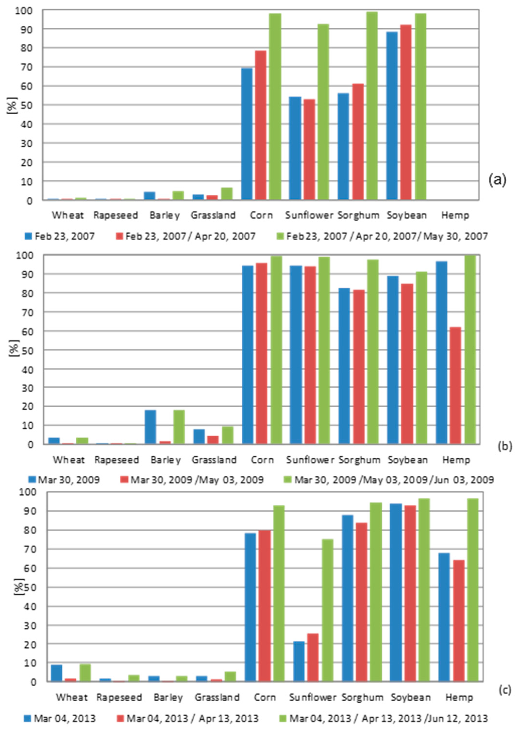
4.2. Chronological Addition of Dates

Table 4. Precision [%] and false positive rate [%] for 1 or 2 or 3 dates (2007, 2009 and 2013).

Years	Dates	Precision [%]	False Positive Rate [%]
2007	Feb-23	64.38	16.06
	Feb-23/Apr-20	82.04	8.88
	Feb-23/Apr-20/May-30	95.17	2.78
2009	Mar-30/May-3	88.75	9.81
	Mar-30/May-3	92.83	6.49
	Mar-30/May-3/Jun-6	98.32	6.68
2013	Mar-4	69.8	13.16
	Mar-4/Apr-13	80.64	10.53
	Mar-4/Apr-13/Jun-12	90.01	4.61

summarizes the quantitative evaluation of the method on the 3 selected years (2007, 2009 and 2013). Whatever the year considered, the addition of images increases the precision. The thresholding of a single date allows between 64% and 88% of summer crops to be detected. This disparity of the results was caused by the fact that the date of the first image in 2007 and 2013 was too early and was exacerbated by the particular climatic conditions in 2013. The closer the dates are to the optimal period (Days 90 to 150), the better are the results. In 2007, the first image was acquired at the end of February when little soil work had been done. The same applied to 2013, when the first image was acquired on 3 March. The use of 2 dates correctly detects from 80% to 92% of the summer crops. The contribution of the 3rd date is crucial, since it increases the summer crop detection rate in June to 90% (2013), 95% (2007) or 98% (2009) and reduces the false positive rate to 4.6% (2013), 2.8% (2007) and 6.7% (2009).

The rate of false positives is also specific to the year in question, decreasing with the addition of images. The variation of values from year to year are mainly explained by the relative chronology between the date of the first available image and the start of tillage on plots (for the single image approach), and by the combination of the satellite images and the calendar of agricultural practices, which can be temporally shifted due to climatic conditions or modified with new cultivation techniques (for the multi-images approach).

The climate variability, shown in Figure 3, has a strong impact on sowing and emergence dates (Figure 2). Summer crop sowing needs to be done in dry, warm soil in order to ensure quick and steady development of the seeds, so that they are less vulnerable to external agents like birds and slugs. In 2013, the cold and rainy weather caused delays in the sowing of summer crops, explaining the lower accuracy (compared to other years).

4.3. Performance Per Crop Type

The performance of the proposed approach was also analyzed for each summer crop type (i.e., corn, sunflower, sorghum, soybean and hemp). The same kind of stratification was applied to winter crops (i.e., wheat, rapeseed and barley) and grasslands in order to study the false positive rate.

Figure 9 shows that the grasslands and the main cultivated winter crops (wheat and rapeseed) are rarely detected as summer crops (rates lower than 8% and 9%, respectively), regardless of the year or the number of images used. For winter crops, the maximum errors are observed in barley for the year 2009. For this year, winter and spring barleys are observed over the monitored plots, and grouped in the same class. However, these two cultivars present distinct phenological cycles: winter barley (which is the main cultivar in the study area) is sown between mid-November and mid-December and spring barley is sown between mid-February and mid-March. Spring barley grows fast and thus presents a high NDVI in spring, which explains the confusion with summer emerging crops.

Regarding the summer crops that are rarely irrigated (hemp, sorghum and sunflower), accurate detection needs three dates (Figure 9). For hemp, this is due to the fact that it is sown in April–May and its cover fraction is high (about 90%, 3 weeks after emergence) with an average NDVI of 0.4. The quality of the detection of hemp depends on the date of the first image and on the time between the first and second dates. Note that no hemp was followed in 2007.

For sunflower, the degraded results observed in 2007 and 2013 (when two images were used), are explained by the date of acquisition occurring before the end of April. At this stage, there are still many plots for which the soil work has not been done yet. For example, in 2013, 10% of sunflower plots were still strongly vegetated (with crop regrowth or self-sown plants). Moreover, sunflower was the crop that was the most affected by the specific climate in 2013 (which resulted in very late planting), and three dates were required to reach 75% of detection in the summer crop class.

In the case of irrigated crops, the rates of detection were less impacted by the year and the specific climate. Corn and soybean were detected as summer crops for more than 75% and 80% respectively, using a single image. Their detection was greater than 90% with three dates, regardless of the year considered.

5. Conclusions

This paper has proposed a method for the early detection of summer crops using a strategy of multi-temporal thresholding of NDVI. The approach is based on the use of optical satellite image time series and was demonstrated using Spot and Formosat-2. A detailed analysis of the phenology of summer crops, winter crops and grasslands could be undertaken thanks to a single dataset combining satellite imagery and in situ data collected over seven years. It enabled an optimal period and a set of NDVI thresholds to be defined, yielding a decision tree for summer crop detection (April to June). During this period, the use of three dates instead of a single image increased the accuracy by 10% to 30% depending on the year.

Using three images acquired at different dates, the precision of summer crop detection ranged from 90% to 99% depending on the climate of the first half of the year and on the actual image availability, but not on the sensor. The availability of data at the optimal dates was crucial for good detection. This simple, robust and reproducible method provided accurate results with the Spot, Landsat, and Formosat-2 missions, and can be implemented with the recent Sentinel-2 satellite or Venμs in the near future. The high temporal repetitiveness of recent missions will increase the opportunity to acquire images during the optimal time period (between Days 90 and 150), and will allow the quick changes of surface states (following a tillage event) to be detected more rapidly. However, for particular years with exceptionally high cloud cover, other approaches based on radar imagery should be investigated.

References

1. Jones, P.D.; Lister, D.H.; Osborn, T.J.; Harpham, C.; Salmon, M.; Morice, C.P. Hemispheric and large-scale land-surface air temperature variations: An extensive revision and an update to 2010. J. Geophys. Res. 2012, 117, 2156–2202. [Google Scholar] [CrossRef]
2. Dore, M.H.I. Climate change and changes in global precipitation patterns: What do we know? Environ. Int. 2005, 31, 1167–1181. [Google Scholar] [CrossRef] [PubMed]
3. Vertès, F.; Jeuffroy, M.-H.; Justes, E.; Thiébeau, P.; Corson, M. Connaître et maximiser les bénéfices environnementaux liés à l’azote chez les légumineuses, à l’échelle de la culture, de la rotation et de l’exploitation. Innov. Agron. 2010, 11, 25–44. [Google Scholar]
4. Jensen, C.R.; Orum, J.E.; Pedersen, S.M.; Andersen, M.N.; Plauborg, F.; Liu, F.; Jacobsen, S.E. A short overview of measures for securing water resources for irrigated crop production. J. Agron. Crop Sci. 2014, 200, 333–343. [Google Scholar] [CrossRef]
5. Houet, T.; Corgne, S.; Hubert-Moy, L.; Marchand, J.P. Approche systémique du fonctionnement d’un territoire agricole bocager. L’Espace Géogr. 2008, 37, 270–286. [Google Scholar]
6. McNairn, H.; Kross, A.; Lapen, D.; Caves, R.; Shang, J. Early season monitoring of corn and soybeans with TerraSAR-X and Radarsat-2. Int. J. Appl. Earth Obs. Geoinform. 2014, 28, 252–259. [Google Scholar] [CrossRef]
7. McNairn, H.; Champagne, C.; Shang, J.; Holmstrom, D.; Reichert, G. Integration of optical and synthetic aperture radar SAR imagery for delivering operational annual crop inventories. ISPRS J. Photogramm. Remote Sens. 2009, 64, 434–449. [Google Scholar] [CrossRef]
8. Waldner, F.; Lambert, M.J.; Li, W.; Weiss, M.; Demarez, V.; Morin, D.; Marais Sicre, C.; Hagolle, O.; Baret, F.; Pierre Defourny, P. Land cover and crop type classification along the season based on biophysical variables retrieved from multi-sensor high resolution time-series. Remote Sens. 2015, 7, 10400–10424. [Google Scholar] [CrossRef]
9. Bastiaanssen, W.G.M.; Molden, D.J.; Makin, I.W. Remote sensing for irrigated agriculture: Examples from research and possible applications. Agric. Water Manag. 2000, 46, 137–155. [Google Scholar] [CrossRef]
10. Seelan, S.K.; Laguette, S.; Casady, G.M.; Seielstad, G.A. Remote sensing applications for precision agriculture: A learning community approach. Remote Sens. Environ. 2003, 88, 157–169. [Google Scholar] [CrossRef]
11. Hadria, R.; Duchemin, B.; Baup, F.; le Toan, T.; Bouvet, A.; Dedieu, G.; le Page, M. Combined use of optical and radar satellite data for the detection of tillage and irrigation operations: Case study in central Morocco. Agric. Water Manag. 2009, 96, 1120–1127. [Google Scholar] [CrossRef] [Green Version]
12. Moran, M.S.; Alonso, L.; Moreno, J.-F.; Mateo, M.P.C.; de la Cruz, D.F.; Montoro, A. A Radarsat-2 quad-polarized time series for monitoring crop and soil conditions in Barrax, Spain. IEEE Trans. Geosci. Remote Sens. 2012, 50, 1057–1070. [Google Scholar] [CrossRef]
13. Fieuzal, R.; Duchemin, B.; Jarlan, L.; Zribi, M.; Baup, F.; Merlin, O.; Hagolle, O.; Garatuza-Payan, J. Combined use of optical and radar satellite data for the monitoring of irrigation and soil moisture of wheat crops. Hydrol. Earth Syst. Sci. 2011, 15, 1117–1129. [Google Scholar] [CrossRef]
14. Marais Sicre, C.; Baup, F.; Fieuzal, R. Determination of the crop row orientations from Formosat-2 multi-temporal and panchromatic images. ISPRS J. Photogramm. Remote Sens. 2014, 94, 127–142. [Google Scholar] [CrossRef] [Green Version]
15. Dabrowska-Zielinska, K.; Inoue, Y.; Kowalik, W.; Gruszczynska, M. Inferring the effect of plant and soil variables on C- and L-band SAR backscatter over agricultural fields, based on model analysis. Adv. Space Res. 2007, 39, 139–148. [Google Scholar] [CrossRef]
16. Duchemin, B.; Hadria, R.; Erraki, S.; Boulet, G.; Maisongrande, P.; Chehbouni, A.; Escadafal, R.; Ezzahar, J.; Hoedjes, J.C.B.; Kharrou, M.H.; et al. Monitoring wheat phenology and irrigation in central Morocco: On the use of relationships between evapotranspiration, crops coefficients, leaf area index and remotely-sensed vegetation indices. Agric. Water Manag. 2006, 79, 1–27. [Google Scholar] [CrossRef]
17. Claverie, M.; Demarez, V.; Duchemin, B.; Hagolle, O.; Ducrot, D.; Marais Sicre, C.; Dejoux, J.-F.; Huc, M.; Keravec, P.; Béziat, P.; et al. Maize and sunflower biomass estimation in southwest France using high spatial and temporal resolution remote sensing data. Remote Sens. Environ. 2012, 124, 844–857. [Google Scholar] [CrossRef] [Green Version]
18. Duchemin, B.; Fieuzal, R.; Rivera, M.A.; Ezzahar, J.; Jarlan, L.; Rodriguez, J.C.; Hagolle, O.; Watts, C. Impact of sowing date on yield and water-use-efficiency of wheat analyzed through spatial modeling and Formosat-2 images. Remote Sens. 2015, 7, 5951–5979. [Google Scholar] [CrossRef]
19. Fieuzal, R.; Baup, F. Estimation of sunflower yield using multi-spectral satellite data (optical or radar) in a simplified agro-meteorological model. In Proceedings of the 2015 IEEE International Geoscience and Remote Sensing Symposium (IGARSS), Milan, Italy, 26–31 July 2015; pp. 4001–4004.
20. Zhu, X.F.; Zhu, W.Q.; Zhang, J.S.; Pan, Y.Z. Mapping irrigated areas in China from remote sensing and statistical data. IEEE J. Sel. Top. Appl. Earth Obs. Remote Sens. 2014, 7, 4490–4504. [Google Scholar] [CrossRef]
21. Pena-Arancibia, J.L.; McVicar, T.R.; Paydar, Z.; Li, L.T.; Guerschman, J.P.; Donohue, R.J.; Dutta, D.; Podger, G.M.; van Dijk, A.; Chiew, F.H.S. Dynamic identification of summer cropping irrigated areas in a large basin experiencing extreme climatic variability. Remote Sens. Environ. 2014, 154, 139–152. [Google Scholar] [CrossRef]
22. Hill, M.J. Vegetation index suites as indicators of vegetation state in grassland and savanna: An analysis with simulated Sentinel 2 data for a North American transect. Remote Sens. Environ. 2013, 137, 94–111. [Google Scholar] [CrossRef]
23. Inglada, J.; Arias, M.; Tardy, B.; Hagolle, O.; Valero, S.; Morin, D.; Dedieu, G.; Sepulcre, G.; Bontemps, S.; Defourny, P.; Koetz, B. Assessment of an operational system for crop type map production using high temporal and spatial resolution satellite optical imagery. Remote Sens. 2015, 7, 12356–12379. [Google Scholar] [CrossRef]
24. Immitzer, M.; Francesco Vuolo, F.; Atzberger, C. First experience with Sentinel-2 data for crop and tree species classifications in central Europe. Remote Sens. 2016. [Google Scholar] [CrossRef]
25. Inglada, J.; Vincent, A.; Arias, M.; Marais Sicre, C. Improved early crop type identification by joint use of high temporal resolution SAR And optical image time series. Remote Sens. 2016. [Google Scholar] [CrossRef]
26. Schwartz, M.D. Phenology: An Integrative Environmental Science; Kluwer Academic Publishers: Dordrecht, The Netherlands, 2003; pp. 3–7. [Google Scholar]
27. Ward, P.R.; Flower, K.C.; Cordingley, N.; Weeks, C.; Micin, S.F. Soil water balance with cover crops and conservation agriculture in a mediterranean climate. Field Crops Res. 2012, 132, 33–39. [Google Scholar] [CrossRef]
28. Fieuzal, R.; Baup, F.; Marais Sicre, C. Monitoring wheat and rapeseed by using synchronous optical and radar satellite data—From temporal signatures to crop parameters estimation. Adv. Remote Sens. 2013, 2, 162–180. [Google Scholar] [CrossRef]
29. Homolova, L.; Malenovsky, Z.; Clevers, J.G.P.W.; Garcia-Santos, G.; Schaepman, M.E. Review of optical-based remote sensing for plant trait mapping. Ecol. Complex. 2013, 15, 1–16. [Google Scholar] [CrossRef]
30. Tucker, C.J. Red and photographic infrared linear combinations for monitoring vegetation. Remote Sens. Environ. 1979, 8, 127–150. [Google Scholar] [CrossRef]
31. Prince, S.D. High temporal frequency remote sensing of primary production using NOAA AVHRR. Appl. Remote Sens. Agric. 1990. [Google Scholar] [CrossRef]
32. Rembold, F.; Atzberger, C.; Savin, I.; Rojas, O. Using low resolution satellite imagery for yield prediction and yield anomaly detection. Remote Sens. 2013, 5, 1704–1733. [Google Scholar] [CrossRef] [Green Version]
33. Latouche, R. Etudes médiévales: Le haut moyen age. La france de l’ouest. Des pyrenees aux alpes. Cah. Civilis. Méd. 1967, 10, 486. [Google Scholar]
34. Durand, Y.; Brun, E.; Mérindol, L.; Guyomarch, G.; Lesaffre, B.; Martin, E. A meteorological estimation of relevant parameters for snow models. Ann. Glaciol. 1993, 18, 65–71. [Google Scholar]
35. Boissard, P.; Pointel, J.G.; Tranchefort, J. Estimation of the ground cover ratio of a wheat canopy using radiometry. Int. J. Remote Sens. 1992, 13, 1681–1692. [Google Scholar] [CrossRef]
36. Denoroy, P.; Justes, E.; Gosse, G. Measuring the rate of soil coverage to estimate the chief characteristics of a colza crop before plant emergence. OCL 2000, 7, 118–123. [Google Scholar]
37. Chern, J.S.; Wu, A.M.; Lin, S.F. Lesson learned from Formosat-2 mission operations. Acta Astronaut. 2006, 59, 344–350. [Google Scholar] [CrossRef]
38. Hagolle, O.; Sylvander, S.; Huc, M.; Claverie, M.; Clesse, D.; Dechoz, C.; Lonjou, V.; Poulain, V. Spot-4 (Take5): Simulation of Sentinel-2 time series on 45 large sites. Remote Sens. 2015, 7, 12242–12264. [Google Scholar] [CrossRef]
39. Rabaute, T.; Tinel, C.; Marzocchi Polizzi, S.; de Boissezon, H. Kalidéos, des images pour la science: Un instrument au service des applications thématiques. Rev. Fr. Photogramm. Télédétec. 2012, 197, 3–9. [Google Scholar]
40. Hagolle, O.; Huc, M.; Villa Pascual, D.; Dedieu, G. A multi-temporal and multi-spectral method to estimate aerosol optical thickness over land, for the atmospheric correction of Formosat-2, LandSat, VENμS and Sentinel-2 images. Remote Sens. 2015, 7, 2668–2691. [Google Scholar] [CrossRef]
41. Pan, Z.; Huang, J.; Zhou, Q.; Wang, L.; Cheng, Y.; Zhang, H.; Blackburn, G.A.; Yan, J.; Liu, J. Mapping crop phenology using NDVI time-series derived from HJ-1 A/B data. Int. J. Appl. Earth Obs. Geoinform. 2015, 34, 188–197. [Google Scholar] [CrossRef]
42. Congalton, R.G. A review of assessing the accuracy of classifications of remotely sensed data. Remote Sens. Environ. 1991, 37, 35–46. [Google Scholar] [CrossRef]
Figure 1. Study site location together with the monitored plots (in orange) and the meteorology points with SAFRAN grid (in green) on a color-composed Spot image.
Remotesensing 08 00591 g001
Figure 2. Mean annual Normalized Difference Vegetation Index (NDVI) phenological cycles (computed during the 2006–2013 period). The blue line represents winter crops and the red line summer crops. Grassland observations are in green.
Remotesensing 08 00591 g002
Figure 3. (a) Precipitations (P) in mm, air temperature (TA) in °C for 2006 to 2013; (b) Precipitations: difference between the monthly average and the monthly average over 8 years; (c) Air temperature: difference between the monthly average and the monthly average over 8 years.
Remotesensing 08 00591 g003
Figure 4. Mean NDVI profiles of all monitored plots for winter crop (blue line), grassland (green line) and summer crop (orange line) for 2006 to 2013. The optimal period (Days 90 to 150) appears in blue, the maximum threshold NDVI value in dark green and the minimum threshold NDVI value in purple.
Remotesensing 08 00591 g004
Figure 5. Examples of observed surface states in early spring: (a) vegetated soil (crop regrowth and self-sown plants); (b) bare soil; (c) emergence; (d) vegetated soil (corn at first phenological stage).
Remotesensing 08 00591 g005
Figure 6. Fraction of soil and vegetated crop plots over the total area representing the monitored summer crops during 2009, 2010 and 2013.
Remotesensing 08 00591 g006
Figure 7. Summary of the rules applied for the summer crop detection (in pink: number of images; in green: conditions; in yellow: surface states and/or agricultural practices).
Remotesensing 08 00591 g007
Figure 8. Time series of surface states of plots cultivated with summer crops in 2010, with an interval of about 10 days between each data point.
Remotesensing 08 00591 g008
Figure 9. Percentage of pixels detected as summer crops: (a) 2007; (b) 2009 and (c) 2013.
Remotesensing 08 00591 g009