Glacier Remote Sensing Using Sentinel-2. Part I: Radiometric and Geometric Performance, and Application to Ice Velocity

Abstract

With its temporal resolution of 10 days (five days with two satellites, and significantly more at high latitudes), its swath width of 290 km, and its 10 m and 20 m spatial resolution bands from the visible to the shortwave infrared, the European Sentinel-2 satellites have significant potential for glacier remote sensing, in particular mapping of glacier outlines and facies, and velocity measurements. Testing Level 1C commissioning and ramp-up phase data for initial sensor quality experiences, we find a high radiometric performance, but with slight striping effects under certain conditions. Through co-registration of repeat Sentinal-2 data we also find lateral offset patterns and noise on the order of a few metres. Neither of these issues will complicate most typical glaciological applications. Absolute geo-location of the data investigated was on the order of one pixel at the time of writing. The most severe geometric problem stems from vertical errors of the DEM used for ortho-rectifying Sentinel-2 data. These errors propagate into locally varying lateral offsets in the images, up to several pixels with respect to other georeferenced data, or between Sentinel-2 data from different orbits. Finally, we characterize the potential and limitations of tracking glacier flow from repeat Sentinel-2 data using a set of typical glaciers in different environments: Aletsch Glacier, Swiss Alps; Fox Glacier, New Zealand; Jakobshavn Isbree, Greenland; Antarctic Peninsula at the Larsen C ice shelf.

1. Introduction

Landsat-type medium-resolution optical satellite sensors are a backbone for operational worldwide glacier mapping and monitoring, and are for instance applied to retrieve glacier outlines, glacier surface facies, or ice velocities [1]. In 2013, Landsat 8 significantly improved the possibilities for glacier observations from space in comparison to Landsat 5 and 7, in particular due to its better radiometric performance (12 bit original, scaled to 16 bit for delivery, compared to 8 bit of Landsat 5 and 7; higher dynamic range; reduced noise level), better geometric stability (pushbroom principle against scanner principle up to Landsat 7), and significantly higher acquisition rate (i.e., higher temporal resolution) due to advanced on-board recording and ground transmission capabilities [2]. The European Copernicus Sentinel-2 satellite series, consisting of two satellites, A and B, may further enhance the worldwide monitoring of glaciers and land ice masses and their changes over time. The first of the satellites, Sentinel-2A, was launched in June 2015, followed by the second satellite, Sentinel-2B, planned for launch in 2016/2017. Both Sentinel-2 satellites operate the MultiSpectral Instrument (MSI).

Among the most important characteristics of MSI for glacier investigations are [3,4]:

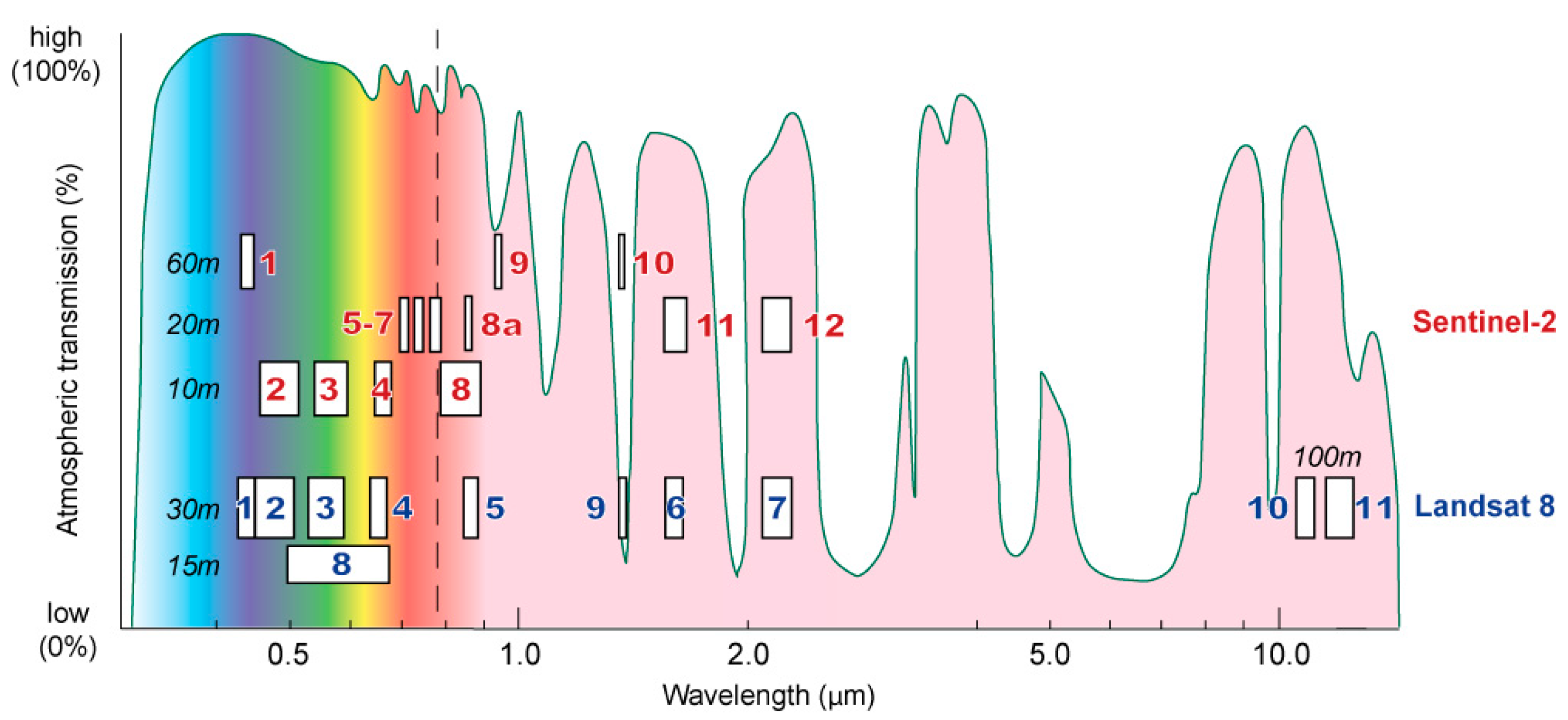
• Four visible and near-infrared (VNIR) bands with 10 m spatial resolution, compared to 30 m (15 m for pan) for Landsat 8 OLI (Figure 1);
• Six VNIR and short-wave infrared bands (SWIR) with 20 m resolution, compared to 30 m for Landsat 8 OLI;
• The Sentinel-2 MSI swath width is 290 km against the 185 km of Landsat 8 (at the cost of larger off-nadir viewing angles and thus larger potential ortho-rectification errors; see Section 3);
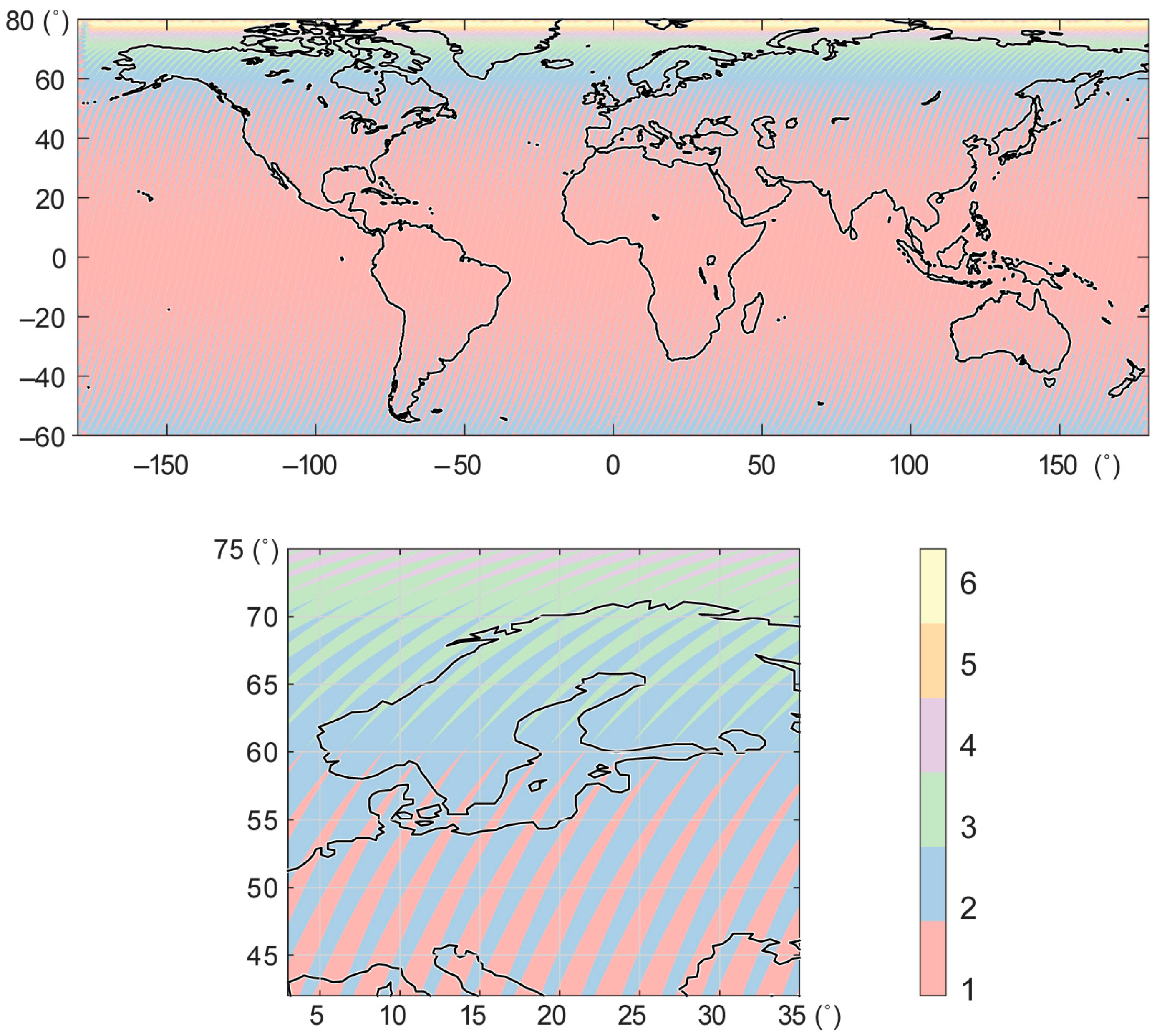
• The Sentinel-2A orbit repeat rate is 10 days against 16 days of Landsat 8, and will become five days from the same relative orbit after the launch of Sentinel-2B. The actual frequency of repeat acquisitions however depends on the capacity of the entire system and the acquisition plan. For higher latitudes where the swaths from neighbouring orbits overlap, the potential revisit time will also be shorter than five or 10 days (Figure 2).
• It should also be noted that Sentinel-2 carries no thermal instrument, in contrast to Landsat 8.

Some performance parameters connected to medium-resolution optical satellite sensors are of particular importance for glacier investigations: automated glacier mapping often relies on VNIR/SWIR band ratios in which thresholds are typically set manually [1,5,6,7]. For such scene-specific segmentation, the relative radiometric precision between individual pixels can be more important than the absolute radiometric accuracy and its stability over time. Also ice velocity measurements, which are typically retrieved by correlating repeat observations, are widely insensitive to absolute radiance calibration variations. They are rather affected by radiometric noise or patterns in the data such as stripes, which reduce accuracy or may even lead to mismatches.

Similarly, the relative geometric precision, i.e., how accurate is the relative geo-location of neighbouring pixels, is of importance for glacier mapping and velocity measurements as it degrades accuracy [8]. This type of geo-location error is also called co-registration accuracy, or co-location accuracy, as it can be estimated from the residuals after co-registering repeat data over the same area.

Absolute geo-location errors, i.e., shifts, rotation, scale, or higher order deformation of an image with respect to true ground coordinates, misplace measurement results and thus affect comparison to data from other sources or between repeat data [9]. The effect of geo-location biases depends on the application, and will be more problematic for mapping glacier terminus changes, where the signal to be observed is of the same order of magnitude as the potential geo-location error, than for displacement measurement points within low-gradient glacier velocity fields, where velocities are very similar within the range of potential geo-location errors.

In part 1 of this paper, we provide first experiences of the Sentinel-2A radiometric and geometric performance with focus on glaciological applications, and demonstrate ice velocities from Sentinel-2. Part 2 of the study [10] focuses on exploitation of the Sentinel-2 spectral content for mapping of glaciers, glacier facies, and other glacier processes. It is important to note that our analyses are based on first Sentinel-2A Level 1C data acquired during the commissioning and ramp-up phases and describe first experiences with Sentinel-2A, and not systematic assessments of larger data volumes acquired over a longer time period. As some image and processing parameters have changed already between both phases (most notably the radiometric scale of the digital numbers provided was increased from 1–1000 to 1–10,000) or might change further, we focus on conclusions that should also hold for the operational phase.

Sentinel-2A Level 1C data consist of radiometrically corrected Top-of-Atmosphere (TOA) reflectance values and are based on a refined geometric model. The raw granules of 25 km cross-track and 23 km along-track from the individual pushbroom modules are mosaicked, ortho-rectified (similar to Landsat 8 data) using a digital elevation model (DEM), and clipped to 100 km × 100 km tiles in UTM projection. The DEM currently used for ortho-rectification of Sentinel-2 is the PlanetDEM 90 (http://www.planetobserver.com; Ferran Gascon, personal communication, 2016), which is “… a multi-source elevation product processed from SRTM data (Shuttle Radar Topography Mission) version 4.1, corrected and completed with many other source data (cartographic, etc.)”. More specific information is not published and not available to us. The DEM used for ortho-rectification of Landsat 8 is a different one, namely the DTED Level 1 from the National Imagery and Mapping Agency (NIMA). Also this DEM is classified with little specific information available [11,12].

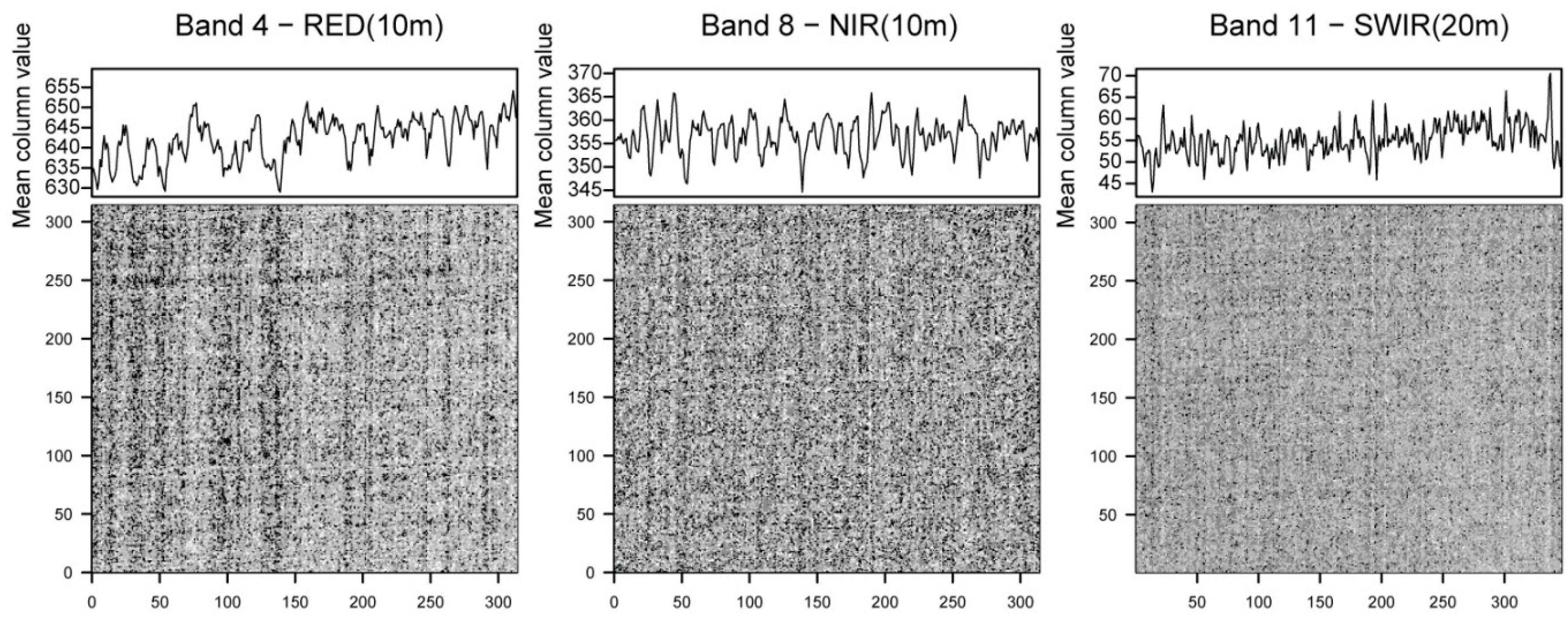
2. Radiometric Noise and Patterns

2.1. Performance over Homogenous Surfaces

Radiometric noise and noise patterns are important quality characteristics of a sensor and may degrade the accuracy of classification results and offset tracking. Here, we provide an initial investigation of the radiometric characteristics from scenes acquired during the commissioning and ramp-up phases of Sentinel-2A and compare them to statistics of Landsat-8 scenes over the same areas. With visual help from higher resolution imagery on GoogleEarth, we carefully selected a number of sites over homogenous surfaces, like water, snow, and deserts, and extracted the standard deviations of DNs over selected small windows (3 × 3, 5 × 5) of these surfaces. For this preliminary radiometric evaluation we used sections of the same scenes used for the other assessments in this study including additional scenes over the Sahara and Tibet plateau containing homogenous sand, snow, or water surfaces. Note, that our analyses below for both sensors are based on a limited number of locations and scenes, and thus form no systematic investigation providing only an order of magnitude for radiometric noise. Sentinel-2 bands 4, 8, and 11 are likely among the most important bands for glacier mapping and offset tracking. Over dark and calm water without sun glint, we find along-track stripes of one pixel in width (confirmed in several scenes at different locations) and on the order of ±7 digital numbers (DN; ±0.0007 Top-of-Atmosphere (TOA) reflectance) for band 4 (Red, 10 m resolution), ±5 DN for band 8 (NIR, 10 m; ±0.0005 TOA reflectance), and ±4 DN for band 11 (SWIR, 20 m; ±0.0004 TOA reflectance) (Figure 3). (Note: the DN values refer to ramp-up phase data where DNs are scaled over a range of 10,000.). These along-track stripes are likely from imperfect de-striping or detector calibration. We also find stripes of similar magnitude in, roughly, the cross-track direction (Figure 3).

For most bright surfaces like firn and snow, we could not observe these patterns. However, we cannot strictly conclude whether the striping is only related to low radiance levels at the detectors, or if the bright surfaces used were simply not homogenous enough to display striping. Occasionally over homogenous bright surfaces, such as Antarctic ice shelves (Section 4.4), we find radiometric differences between the individual swaths of the 12 pushbroom modules that form the Sentinel-2 focal plane on the order of 30 DN (±0.0030 TOA reflectance). Most likely, these differences derive from different gain settings or radiometric offsets between the pushbroom modules (cf. below Section 3.1 and Section 3.2 for geometric offsets between the modules). Most glaciological applications will be little affected by this kind of striping on the order of 4–7 DNs (0.0004–0.0007 TOA reflectance), perhaps with the exception of glacier mapping in dark shadow areas. Potentially, the stripe patterns could be removed by improved calibration procedures within the processing system or by additional empirical de-striping by the user.

For medium-bright homogenous surfaces, such as in deserts, we see a random radiometric noise level on the same order as the above stripes (~±5 DN; ±0.0005 TOA reflectance), for bright snow and firn areas (accumulation areas) even less. For comparison, noise levels of Landsat 8 DNs are on the order of 30 DN for bands 4, 5, 6, and 8 (red, NIR, SWIR, 30 m, and pan, 15 m; 0.0006 TOA reflectance), and no stripes are detectable on dark surfaces. Landsat 8 DNs are scaled to 16 bit (65,536) and their noise level translates to similar values as for Sentinel-2, as also seen from the respective TOA reflectance values. As natural variations of reflectance over the test surfaces are to be expected, the above noise estimate is a conservative maximum one. It is important to reiterate that these analyses represent an initial rough test and are not systematic and statistically extensive.

The effect of the noise described above on band ratios, which is the most established method for automatic mapping of ice surfaces [1,10], is on the order of 1%. For instance, the resulting uncertainty of a threshold of 2.0 for typical mapping conditions (called ‘th1’ in [10]) becomes ±0.015, which is far below the uncertainty of manually setting and adjusting this threshold, as is usually done. The effect of the above radiometric noise on multispectral analyses and offset tracking seems negligible to us and by far smaller than uncertainties stemming from varying glacier properties and imaging conditions.

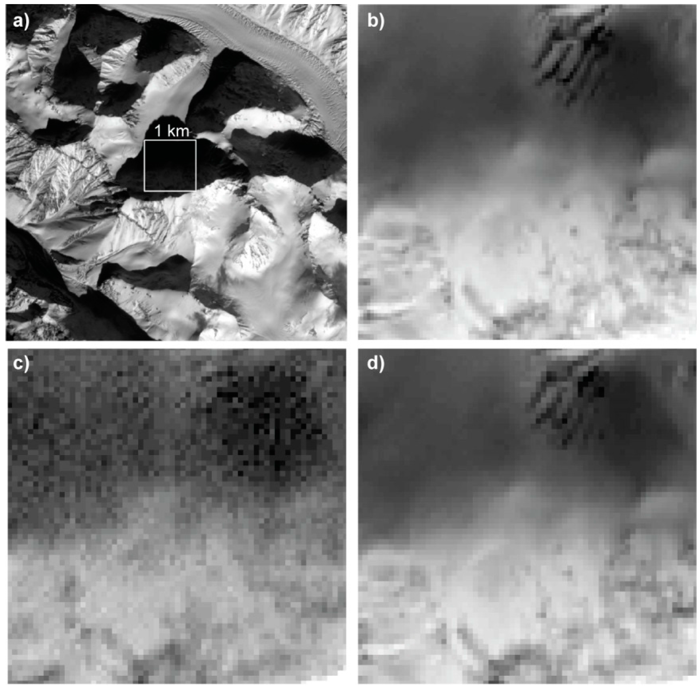
2.2. Performance in Shadows

Glaciers are often situated in mountains with rugged topography so that the radiometric performance of an optical sensor in mountain or cloud shadow areas is important for achieving maximum coverage of glacier mapping and velocity measurements. Figure 4 shows a deeply shadowed mountain flank seen through Sentinel-2A, Landsat 7 and 8. This example, and other similar tests confirm that ground details in shadow areas become well visible through the original 12-bit radiometric resolution of Sentinel-2 MSI (and Landsat 8 OLI), in strong contrast to 8-bit data such as from Landsat 7 ETM+ or ASTER. This improved performance in shadows is important for glacier mapping as it can reduce problems within multispectral classification of ice and snow (see part 2 of this study, [10]). In the 12-bit images, offset tracking over glacier sections in cast shadow performs almost as well as outside of the shadows, in contrast to 8-bit images where tracking typically fails completely in shadow areas. Only the shadow boundaries themselves cause problems in the 12-bit data as they represent a dominant visual contrast so that shadow margins are tracked between repeat images, instead of the often weaker glacier surface features.

The example in Figure 4 used bands with the highest resolution of the respective sensors as these will typically be used for displacement measurements. As the resolution of these bands is not the same, and the bands compared do not cover the same spectral range, Figure 4 cannot be considered strictly a direct comparison. A comparison of bands with similar spectral ranges is given in part 2 of this study [10].

Similarly to shadowed areas, the original 12-bit radiometric resolution for Sentinel-2 data (and also Landsat 8, though delivered as 16 bit) also avoids radiometric saturation over bright snow and firn surfaces, which was a common problem and limiting factor for using 8-bit images over glaciers and snow [7]. The higher dynamic range and radiometric resolution are of great benefit for offset tracking over snow and ice surfaces. Studies on mapping and characterizing ice and snow surfaces will be enhanced by the strongly increased level of radiometric detail, for instance mapping of snow lines or snow/firn/ice properties, albedo changes, and/or time series analyses [7,13].

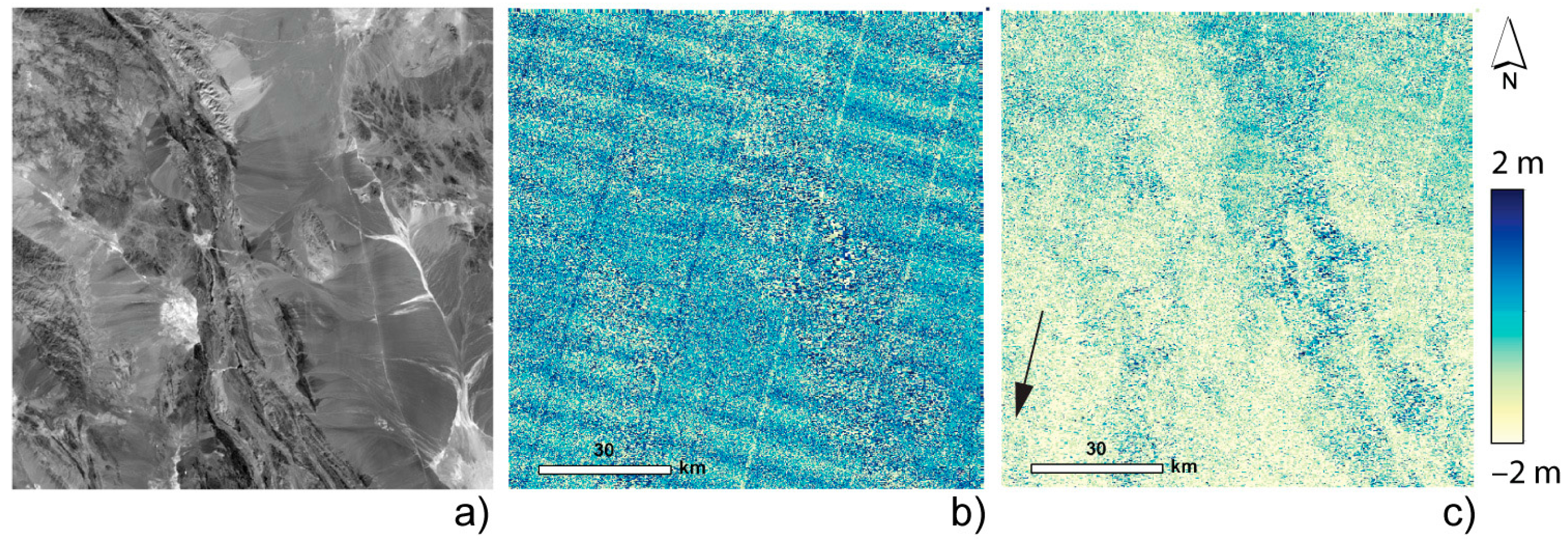
3. Geometric Performance and DEM Effects

The geometric performance of Sentinel-2A data in view of glacier applications can be separated into three error-budget terms:

(i)

The relative geo-locational precision between different images, also called co-registration accuracy. This group of errors can be random (i.e., noise) but also contain systematic patterns such as attitude jitter or calibration errors. (The latter error patterns could also be seen as higher-order components of the following error category, ii.)

(ii)

Mainly shifts, but also rotation or deformation, apply to entire scenes and are scene-specific or system-specific geo-location biases in the image data with respect to the true ground location of the measurements. Typically, these biases stem from errors or inaccuracies in spacecraft attitude or position measurements or in the subsequent solution of the image orientation parameters.

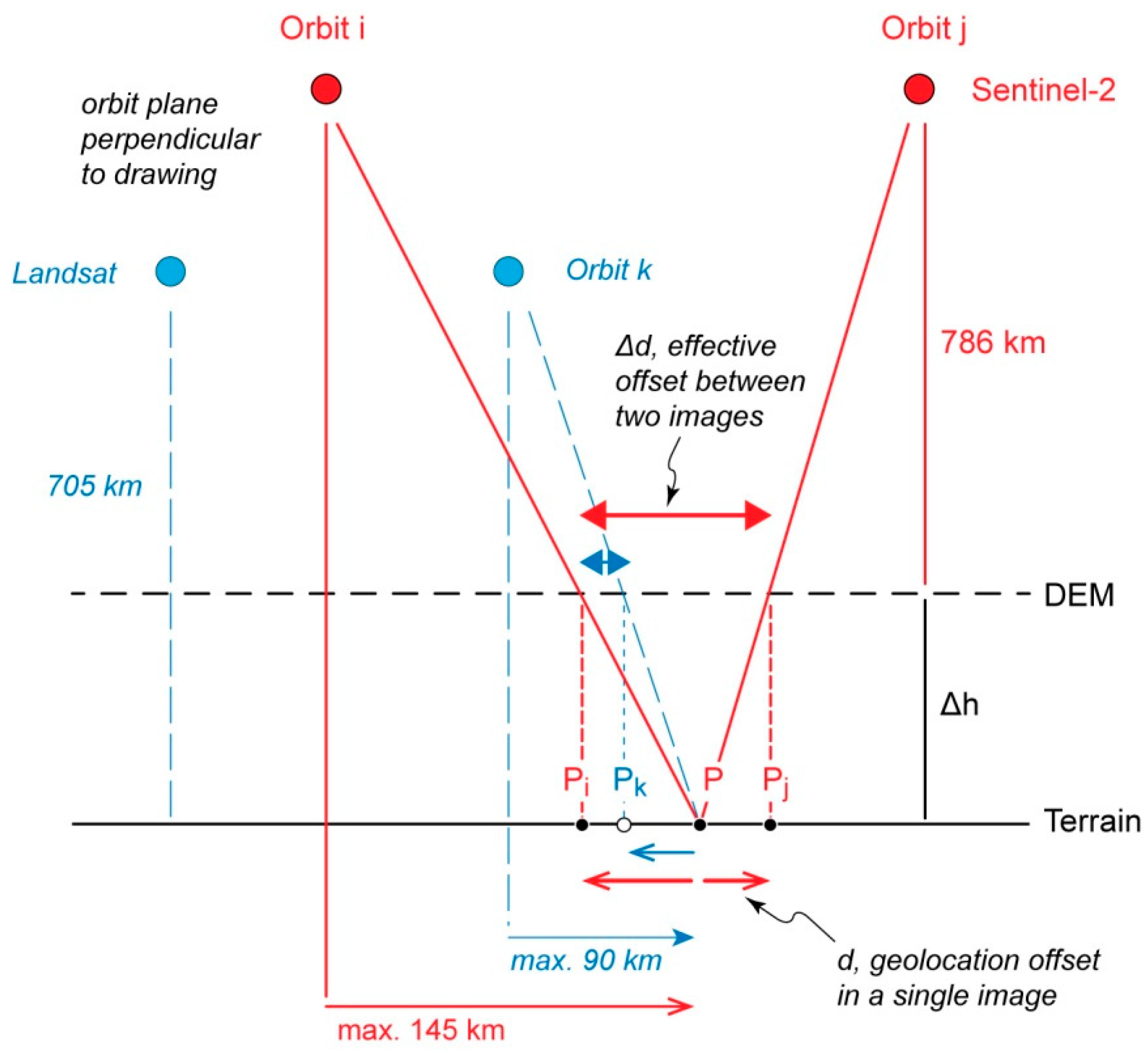
(iii)

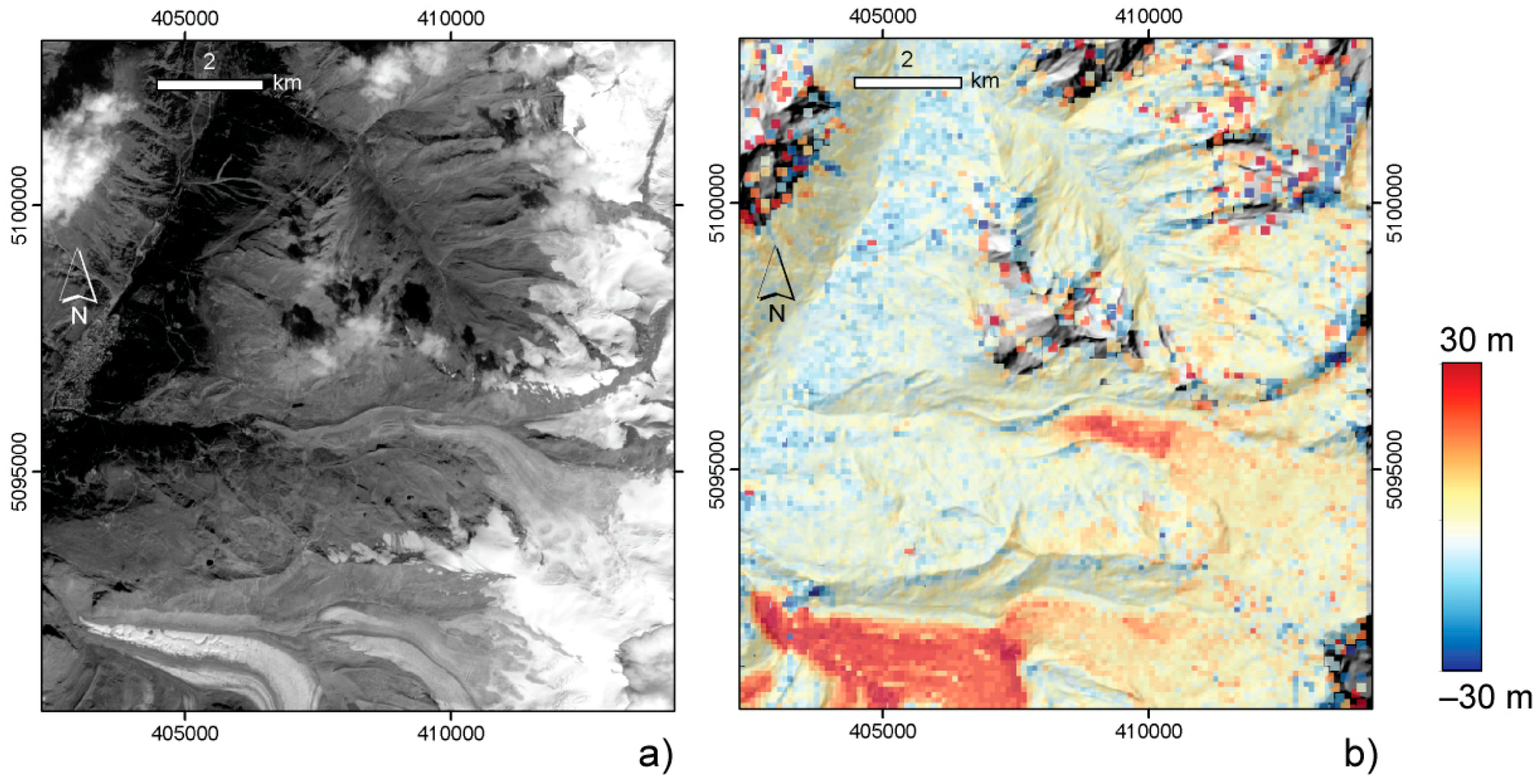
Of large practical significance for glacier and high-mountain applications, vertical errors in a DEM elevation used for ortho-rectification or terrain correction of the raw data propagate into a pattern of local horizontal off-nadir offsets in the ortho-rectified products such as Landsat L1T or Sentinel-2 L1C. The effect of these elevation errors depends on the off-nadir view angle, in particular in cross-track direction, and the magnitude of the elevation error (Figure 5). The maximum off-nadir distance d of a point in a Sentinel-2 scene can be 145 km (i.e., half the swath width) so that a vertical DEM error Δh translates in the worst case into a horizontal geo-reference offset in cross-track direction of

$$d_{max\left(S2\right)}\approx \mathsf{\Delta }h/5.4$$

(1)

by dividing the flight height by the maximum off-nadir distance (or half the swath width). The respective ortho-rectification offset in a Landsat scene can be roughly up to

$$d_{max\left(Landsat\right)}\approx \mathsf{\Delta }h/7.8.$$

(2)

When comparing two orthoimages from orbits on different sides of a ground point zenith, the above ortho-rectification offsets in cross-track direction accumulate. For instance, in Figure 5, when comparing an orthoimage from orbit i with one from orbit j, the offset between projections Pi and Pj of ground point P becomes visible. The maximum relative offset Δd between two Sentinel-2 scenes from neighbour orbits is reached for a point where the margins of two neighbour swaths intersect and is double the maximum offset in a single scene:

$$\Delta d_{max\left(S2\right)}\approx \mathsf{\Delta }h/2.7.$$

(3)

In practice, whether these cross-track offsets appear and need to be accounted for depends upon the orbit pattern and latitude, and whether it is necessary to use data from neighbouring orbits instead of only one, i.e., due to for example cloud cover or a rather large change rate on the ground. Figure 2 provides an impression of the Sentinel-2 swath pattern and thus the distribution of respective overlaps. Only the difference of the two individual offsets becomes effective if the two orbits are on the same side with respect to a ground point zenith, e.g., offset Pi–Pk in Figure 5 becomes visible.

Two types of errors contribute to vertical offsets (Δh) between the terrain and its approximation by a DEM: (a) measurement or production errors where DEM elevation does not agree with terrain elevation at the time of acquisition of the elevation data; and (b) changes in terrain elevation over time between elevation measurement and satellite scene acquisition. For glaciological applications, the most prominent DEM error of type (b) is due to real glacier elevation changes, which can amount to tens or even hundreds of metres depending on the age difference between the DEM and satellite image. It is beyond the scope of this contribution to discuss the DEMs used for ortho-rectification of Sentinel-2 or Landsat data as both DEMs are classified (i.e., not available to the public), however it is clear that DEM error type (a) can reach the same order of magnitude as type (b).

The three horizontal bias categories described above (i, overall scene offsets; ii, higher-order offset patterns; iii, ortho-rectification offsets due to DEM errors) are superimposed with each other but can be partially isolated by special experimental setups.

3.1. Co-Registration of Data from Repeat Orbits

When co-registering two repeat orthoimages acquired from the same relative orbit (repeat orbit), DEM effects will be present but have the same pattern in both data sets so that they become mostly eliminated in the offset field obtained from correlating the two images. The final offset field contains thus differential geo-location noise and biases of higher orders such as shifts, jitter, etc. For related experiments we choose scenes with good visual contrast for matching and little surface changes expected, conditions often offered by deserts. We use standard normalized cross-correlation to track offsets [14,15,16].

From tests based on repeat Sentinel-2A commissioning and ramp-up phase data (band 8, NIR) over the Sahara and over the border region between Afghanistan and Iran we find mean offsets (i.e., biases) on the order of 1–3 m in each cross-track and along-track direction, in some cases up to 10 m in the along-track direction. The standard deviation of these mean biases (i.e., the random component of co-registration) is on the order of ±1–2 m. For the limited number of co-registration tests performed in this study, the distribution of offsets seems close to Gaussian, for some cases slightly more narrow (see Section 3.2), so that the standard deviations calculated provide rather conservative estimates of co-registration accuracy, roughly the third quartile, 75%. Some of the co-registration tests reveal offset patterns, in both the along- and cross-track directions. These patterns result mostly from misalignments in the overlap areas of the 12 adjacent pushbroom modules that cover the 290 km swath of Sentinel-2 (Figure 6), and more seldom jitter undulations (vibrations in attitude angles) with a ~7–8 km wavelength (the distance between maximum offsets in flight direction, Figure 7, middle panel) and an amplitude on the order of 1 m (Figure 7). In the few cases where jitter was found, it was mainly seen in the along-track component. These offset patterns, such as jitter, visible in the co-registration represent the sum of two individual patterns, from the first and the second image respectively. The superposition of the two patterns (e.g., wave patterns in the case of jitter) can be a destructive or constructive interference [8]. For instance, even if present in both scenes co-registered, the resulting amplitude can be reduced, or it can be exaggerated (doubled in maximum) in the offset fields between both scenes. Thus, it is not possible to draw conclusions about the original jitter from two scenes alone.

In sum, the co-registration accuracy found for the Sentinel-2A data investigated is on the order of 1/10 of a 10 m pixel. Typically, this order of precision is close to the matching accuracy achievable so that parts of this estimate could actually be due to matching inaccuracies rather than Sentinel-2A geo-location noise. In order to better quantify and characterise the biases and offset patterns found, a systematic and dedicated study with significantly more data over more test sites would be necessary. Co-registration of 20 m-bands was not investigated here, as they will be less likely used for displacement measurements. As the detector lines for the 10 m-bands and the 20 m-bands are rigidly connected on the same focal plane, we expect the same co-registration characteristics.

To our knowledge, future Sentinel-2 processor versions plan to register new scenes to a reference scene or scene composite from the same relative orbit (Ferran Gascon, personal communication, 2016). This measure would largely remove the above co-registration biases, but could also remove parts of the higher-order offset patterns seen, depending on the co-registration model applied.

For reference, we also performed similar co-registration studies for band 8 (pan, 15 m) of Landsat 7 ETM+ and Landsat 8 (Figure 8). From several scenes over the Kelso area in California we found mean co-registration biases of around 1–1.5 m with a standard deviation of ±3–4 m, both in along- and cross-track directions for Landsat 7. Biases of 1 m with a standard deviation of ±2.5–3 m are found for Landsat 8. Strong cross-track undulations were found for Landsat 7 co-registrations, likely composed of several wavelengths with a shorter one around 30 km in flight direction, an amplitude of ±2–3 m, and a combined amplitude of the offsets around ±5 m (Figure 8, middle panel). This pattern could result from a kind of jitter related to the scanner principle of this instrument against the pushbroom principle used for Landsat 8 and Sentinel-2.

Again and as for all tests presented in Section 3, the sample size behind this assessment is limited and does not necessarily reflect an average performance of Landsat 7 and 8. We also would like to stress that most test areas within Section 3 are situated in mid to low latitudes and that the offset patterns found are thus not necessarily representative for high latitudes, for instance due to the different orbit azimuth with respect to the Earth’s rotation axis.

As a side-note, in many of the co-registration patterns investigated over arid landscapes (Sahara, Iran, Australia), we find also patterns that match natural surface patterns (for example, Figure 7, right panel, blue offset area to the top middle). These offsets of up to several metres are especially found over dry sandy areas, and for instance not over bedrock, and thus we speculate that these offset patterns could stem also from small vertical offsets Δh in the SRTM elevation model directly due to penetration of radar waves into the sandy dry soil [17] or due to local SRTM DEM shifts due to this penetration. (The SRTM DEM is incorporated in the DEM used for Sentinel-2 ortho-rectification; see Section 1). Even if the data compared are from the same relative orbit, small differences in viewing directions could cause small-baseline stereo effects leading to horizontal offsets, Δd, as described in Section 3. Such small-angle stereo effects are also involved in the process of focusing the different bands and pushbroom modules onto the ground. Note that only offset differences, Δd, between both co-registered scenes become visible in such cases (Figure 5). Also, we cannot completely rule out terrain movements between the two acquisitions such as from dune migration [18,19] or shadow movements, though visual image inspection does not support these possibilities.

3.2. Co-Registration of Data from Neighbouring Orbits

When co-registering repeat data sets from neighbour orbits, the vector sum of two horizontal projections of vertical DEM errors becomes visible in addition to the relative and absolute geo-location errors described in the above section. DEM errors and thus their horizontal propagation into ortho-rectified data are expected to be particularly large for mountain areas with steep slopes or where the DEM source data are of reduced accuracy in general. As a special case over glaciers, DEM elevations are almost by necessity outdated with respect to the time of image acquisition, unless simultaneous stereo data are available (e.g., for ASTER or SPOT5). Such elevation differences will typically be largest at the glacier termini. When using repeat data over glaciers the detection of DEM errors is complicated by the fact that ice motion vectors are superimposed over the DEM error projections (see Section 4.1), unless ice motion is negligible over the observation period.

No specific DEM source information is available for PlanetDEM 90 (the DEM used for ortho-rectification of Sentinel-2 data) north of the SRTM extent. A DEM source that is, however, publicly available for large areas outside the SRTM is the various DEMs provided through www.viewfinderpanoramas.org, which is among others based on Soviet Union cartographic maps. In order to test if this DEM is used for Sentinel-2 ortho-rectification for a test site in Northern Norway (i.e., outside of the SRTM coverage), we difference the DEMs from the Norwegian mapping agency (Statens kartverk) and from www.viewfinderpanoramas.org. Figure 9, left panel, shows vertical differences between both DEMs of many tens of metres, sometimes even as much as 100–200 m. We then calculate the horizontal offsets between Sentinel-2A scenes acquired on 18 August and 22 August 2015 during the relative orbits R051 and R008, respectively. The test area lies between the two ground-projected orbit tracks, roughly 45 km away from each of them in both directions, and thus the orbit tracks have a cross-track distance of about 90 km from each other (case Pi–Pj in Figure 5). For each of the two images, vertical DEM errors propagate into horizontal offsets (d) with a ratio of about Δh/17.5, and the total effective offset between the two images Δd becomes Δh/8.7. Scaling the horizontal offsets measured between the two Sentinel-2A scenes with this factor, we reconstruct the elevation errors Δh that correspond to the horizontal offset field (Figure 9, right). In fact, the reconstructed Δh appears very similar to the actual Δh of the DEM by www.viewfinderpanoramas.org, suggesting that the latter DEM is in some way part of the conglomerate DEM used for Sentinel-2 ortho-rectification, at least over Norway, where we found similar results also for other regions and orbit tracks. The study area in Figure 9 is close to the orbit tracks (45 km). At the image margins (i.e., 145 km off-nadir), elevation errors of 100–200 m would translate into georeference offsets d_max of 18–37 m in one scene, and of up to 37–74 m between scenes from different orbits (Δd_max, Equation (1)). Similar tests performed with Landsat 8 scenes with cross orbits of ~50 km do not show similarity with the elevation differences of Figure 9 and reconstructed DEM errors of up to ~50–60 m imply the use of a more accurate DEM than the one used for Sentinel-2. In summary, by reconstructing DEM errors in this way, we are able to identify the source of the classified DEM used for ortho-rectification and characterize it to better understand and a priori estimate lateral offsets in the orthoimages due to DEM errors and changing topography between the DEM and image dates.

To expand our investigation of Sentinel-2 L1C image co-registration from overlapping neighbouring orbits, we select ice free areas on the west coast of Greenland and measure offsets by cross-correlation. Moving areas like glaciers, ice sheet, and the ocean were masked out using the Randolph Glacier Inventory Version 5.0 [20] and the GIMP ice and ocean mask [21]. The two data sets of relative orbit R68 and R111 were acquired on 16 August and 9 September 2015 (Figure 10). The histograms of displacements for stable terrain indicate a mean mis-location of −2.1 m and +3 m with a standard deviation of 3.8 m and 2.6 m in Easting and Northing, respectively, corresponding to 0.2 and 0.3 pixels of band 8. The histogram spread is mostly caused by DEM errors propagating into the ortho-rectfication of the images from different orbit tracks. Note that due to orbit azimuth, cross-track offsets from DEM errors propagate both into the Easting and Northing coordinates, though predominantly into Easting at the latitude of this test area (see Section 4.3). When transformed to the track direction (116° azimuth) we obtain a mean cross-track displacement of −0.6 ± 4.5 m and an along-track component of 3.6 ± 0.75 m, confirming that the standard deviation is largest in cross-track direction due to DEM errors.

Within the coverage of SRTM, vertical DEM errors are generally expected to be smaller than outside SRTM. In addition, larger errors over steep and glacierised mountains are expected where SRTM voids are common (see Section 3.3; at this point, we do not know how SRTM voids are filled in the PlanetDEM 90). As a result, cross-track offsets between Sentinel-2A data from different orbits on gentle terrain within SRTM coverage are substantially smaller than the offsets found for instance in Northern Norway (Figure 9). In this manner, the reduced terrain-induced error helps expose other biases and effects. Several test sites over flat desert environments at mid and low latitudes reveal cross-track offset patterns similar to Figure 11. The overlay of the cross-track offsets between different pushbroom modules from both individual overlapping scenes (such as in Figure 6) can be destructive or constructive, as in the case here, with offsets between pushbroom module swaths of 5 m or more. In addition, there seems to be a slight along-track tilt between both scenes. In the northern section of Figure 11, we find abrupt cross-track steps in the offsets, perhaps from steps in the DEM used for ortho-rectification, or from processing artefacts. For the offsets in Figure 11, we find a mean cross-track offset of 0.7 ± 1.7 m, and an along-track offset of 21 ± 1.7 m (not shown).

Similar tests at the same sites were performed for the overlaps of Landsat 8 scenes taken from neighbouring orbits. Cross- and along- track offsets are found to be around 1 ± 3 m and 1.5 ± 2.5 m, respectively. As with Sentinel-2 MSI, slight along track tilt and along-track stripes from the individual Landsat 8 push-broom modules become visible, on the order of 3 m but with less clear boundaries.

3.3. Co-Registration between Sentinel-2A and Landsat 8 Data

As Sentinel-2A and Landsat 8 orbits are not equivalent, comparison of images from both satellites resembles the analysis in the previous section but with some differences. Mainly, the geometric setting between the Sentinel-2A and Landsat 8 orbits is different and the ortho-rectification of data from both systems involves DEMs that are different, at least in parts, so that the expected offsets between repeat data from Sentinel-2A and Landsat 8 are different to offsets in data from neighbour Sentinel-2 orbits. As Sentinel-2 and Landsat 8 data will most likely be combined in many glacier remote sensing studies, this offset experiment is of as high practical relevance as the comparison for Sentinel-2 data from neighbour orbits. To test this, we find near-simultaneous and overlapping Sentinel-2 and Landsat 8 acquisitions so that the ice movement and surface change components in the offsets become negligible, which would otherwise complicate direct comparisons.

Over the Swiss Alps, we match offsets between a near-simultaneous Landsat 8 and Sentinel-2 pair acquired on 8 September 2015 (~20 min apart; Figure 12). The Landsat 8 pan data is resampled to the 10 m resolution of Sentinel-2A band 8 using bi-cubic interpolation. Maximum cross-track offsets of 20–30 m appear over the glacier tongues. The test site lies in between the Landsat 8 and Sentinel-2 orbit ground tracks with cross-track separation from image nadir of 80 and −65 km, respectively. In the case that Landsat 8 and Sentinel-2 data were orthorectified using the same DEM, horizontal offsets d in both images would sum up to Δd ≈ Δh/5.1, corresponding to DEM errors of 100 m to 150 m. We do not know for certain whether the SRTM DEM is part of the DEMs used for ortho-rectifying Sentinel-2 and Landsat 8 data over the study site. Elevation losses on the order of 100 m between the 2000 SRTM DEM and 2015 have been measured [22], suggesting that an outdated DEM has been used for the orthorectification, and possibly the same DEM, such as the SRTM. Outside of the glaciers, offsets are on the order of a few metres with some spatial patterns, likely due to systematic vertical errors of the DEMs used for ortho-rectification, for instance over forest, steep terrain, and/or void fills.

3.4. Co-Registration to Reference Images

A final experiment to test the relative and absolute geo-location accuracy of Sentinel-2A data is their correlation with reference images. Here, we use the swissimage25, a 25 m version of a national airborne orthophoto based on aerial photos of 2009–2011, as a reference image to track offsets between the Sentinel-2 tile T32TMS from 29 August 2015 and the Landsat path 195 row 28 image from 30 August 2015. The reference image is resampled (bicubic) to 20 and 30 m for matching it with Sentinel-2A band 4 and Landsat 8 band 4, respectively. For the Sentinel data, we obtain a mean Easting offset of 12 ± 8 m, and −24 ± 7 m in Northing. For the Landsat data 13 ± 9 m in Easting and −2 ± 7 m in Northing. While the offsets for Landsat are boarder-line significant, the Northing offset for the Sentinel-2 tile is in line with occasional along-track offsets of 10 m or more suggested by above tests (Section 3.1). However, these comparisons are not strict and provide only an indication of geo-location accuracy because (i) the reference image has a lower resolution of 25 m; (ii) the pixel aggregation processes from the original meter-resolution airphoto mosaic to 25 m are different to the spatial-spectral mixing processes within a Sentinel-2 or Landsat 8 pixel; and (iii) the time span between both data sets that particularly disturbs matches in the mountains due to snow cover variations. The geo-location accuracy of the reference image mosaic swissimage25 is on the order of 3–5 m (www.swisstopo.ch), which also contributes to offset magnitudes in our Sentinel and Landsat data. It is therefore not easily possible to separate all offset influences. Nonetheless, this confirms the geo-location accuracies estimated in the tests above using an independent method.

4. Ice Velocity Measurement

The high spatial resolution of up to 10 m together with the high repeat rate between 10 and a few days (dependent on latitude), would make Sentinel-2A and then later Sentinel-2B suitable for worldwide measurement of glacier motion, both alone and in combination with Landsat 8. Ice dynamics, together with the climatically-driven surface mass balance, is a key process forming glaciers and therefore a crucial glacier and climate variable [1]. Changes in ice flow can be responsible for large and fast glacier mass changes [23], may pose hazards [24], or help to understand the potential reaction of glaciers to climatic changes [25].

Here, we use standard cross-correlation techniques between repeat Sentinel-2A and Landsat 8 data to track the offsets of visual features over time [14,15,16,26]. The aim is to explore the general potential of Sentinel-2A for ice velocity measurement, among others compared to or in combination with Landsat data. We do not develop specialized algorithms for Sentinel-2.

4.1. European Alps

For Aletsch Glacier, Swiss Alps, we track displacements from Sentinel-2A band 8 data from 30 July and 8 September 2015, i.e., over 40 days, from the same relative orbit R108 (Figure 13a). Speeds reach up to 0.8 m/day in an icefall from the Ewigschneefeld glacier. Velocities tracked over 7 August–8 September (32 days; both images path 194 row 28) from repeat Landsat 8 band 8 data are shown in Figure 13b. In most parts of the glaciers the Sentinel-2 derived velocity field is more complete with less outliers after application of the same correlation threshold. Visual comparison of image details suggests that this is due to the higher resolution of Sentinel-2 that is able to depict finer details than Landsat 8 so that the image cross-correlation is slightly more successful. The reduced coverage of Sentinel-2 offsets compared to Landsat 8 offsets in the Ewigschneefeld ice fall to the upper middle of the Figure 13 panels is likely due to melt of snow patches between 30 July and 7 August. Note that the use of different spectral bands in our comparison might influence matching differences (Sentinel-2: NIR band 8; Landsat 8: VIS pan band 8; [27,28]). The velocities obtained here agree well with other measurements [29,30].

We also tracked displacements between the Landsat (7 August) and Sentinel-2 (8 September) after resampling the Landsat 8 band 8 data to the Sentinel-2 band 8 resolution of 10 m using bi-cubic interpolation. As the two images are not acquired from the same orbit but at off-nadir distances of −80 km and 65 km from the Landsat 8 and Sentinel-2 ground tracks, respectively, effective offsets Δd between both scenes due to DEM errors become approximately Δh/5. Consequently, the cross-track offset components Δd from DEM errors on the Aletsch Glacier dominate the velocity field, so that the cross-track offsets (roughly in east–west direction; E–W) sum up with the ice flow vectors (roughly NW-SE) to NE-SW vectors (Figure 13c).

Besides this effect, ice velocity tracking between the Landsat and Sentinel-2 scenes (7 August–8 September 2015) seems to provide slightly more successful matches than the tracking between Landsat only (7 August–8 September 2015). We are not sure about the reason behind this effect, and a further systematic and detailed study is required to confirm it for other sites and times and to further understand it. The higher level of detail in the second image (Sentinel-2) could lead to slightly better correlations and/or the spectral range of the Sentinel-2 band 8 (NIR) might be better suited than that of Landsat 8 pan (VIS; stronger atmospheric effects?). This effect could also be a random result from, for instance, slightly more suitable atmospheric or illumination conditions at 10:30 UTC (Sentinel-2) than 10:10 (Landsat 8) or a more suitable viewing angle, for instance with respect to atmospheric effects. In this example, combination between Landsat and Sentinel-2 data for ice velocity measurements could be beneficial, while errors in the DEMs used for ortho-rectification of the data bias the results strongly reducing or removing the potential for glacier velocity measurements.

Velocity vectors between the repeat data from same orbits (Figure 13a,b) are not affected by ortho-rectification offsets, but the geo-location of the measurements is actually offset by d (Equations (1) and (2)), i.e., reaching magnitudes of tens of meters depending on the DEM errors Δh and the off-nadir distance of the locations. This effect will typically not be visible and will shift result locations similarly since the same outdated DEM is used. However, due to the fact that the offsets d will often vary systematically over a glacier with elevation errors Δh increasing from the accumulation areas towards the glacier tongues (Figure 12), it might be necessary to observe this effect for special analyses, for instance velocity change detection.

4.2. New Zealand

In order to test the performance of Sentinel-2A derived ice velocities over a fast-flowing, maritime (and thus sensitive) mountain glacier, we track displacements over Fox Glacier, New Zealand [31,32] from 3 Sentinel-2A images (24 December 2015—3 January 2016—13 January 2016; Figure 14). Displacements were measured in all three combinations, i.e., two subsequent 10-day periods and the full 20-day period, and the residual $\overrightarrow{\mathsf{\epsilon }}$ of the vector sum triangulated for each location:

$$\overrightarrow{\mathsf{\epsilon }}={\overrightarrow{d}}_{12}+{\overrightarrow{d}}_{23}-{\overrightarrow{d}}_{13},$$

(4)

where $\overrightarrow{\mathrm{d}}=\left(\text{dx},\text{dy}\right)$ is the two-dimensional horizontal displacement vector between times 1 and 2, 2 and 3, and 1 and 3, respectively. The lengths of the residual vectors $\overrightarrow{\mathsf{\epsilon }}$ and low correlation coefficients were used to mask out potential outliers. Both these parameters exhibit a similar pattern and are thus useful to mask out most erroneous measurements automatically (Figure 14). We suggest that the arbitrary thresholds used here (10 m for triangulation sum and 0.6 for correlation coefficient) are specific to the scene contents and imaging conditions, and thus future applications may require individual calibration. The large majority of the residuals (~80%) are 1–2 m in length ($\left|\mathsf{\epsilon }\right|=\sqrt{{\mathsf{\epsilon }}_{\mathrm{x}}^2+{\mathsf{\epsilon }}_{\mathrm{y}}^2}$). This number suggests that over few repeat orbits, i.e., short times that limit glacier surface changes, ice displacements from Sentinel-2 can be measured with a precision of 10%–20% of a 10-m pixel even over fast flowing and fast changing medium-size maritime glaciers.

In principle, the glacier displacements measured are composed of the real ice movement, differential geo-location, and higher-order biases (Section 3.1). The fact that the triangulation residuals of 1–2 m found here are of the same size or even better than those potential biases indicates that these effects were, in this example, either small or cancelled out by affecting all images matched in the same way (i.e., destructive interference).

Figure 14 shows the ice velocity on Fox Glacier from 24 December 2015–3 January 2016 revealing two strong ice flows from the accumulation area, and a weaker one to the south that coalesce at roughly the same place and reach then maximum speeds of 4.5 m/day below the main ice fall of Fox glacier (see also [32]). Significant speed increases between the two subsequent 10-day periods of up to 1 m/d over 10 days were observed, corresponding to an acceleration of up to 20%. Most of this increase seems to have happened on the middle, main ice flow (Figure 14, lower panel). Such changes in speed are completely realistic according to ground measurements, and could be due to heavy rain events, for example [34]. These results demonstrate how the high accuracy of the displacements, as suggested based on the triangulated vector-sum residuals, can be applied to quantify ice velocity changes even over short time intervals of days or weeks.

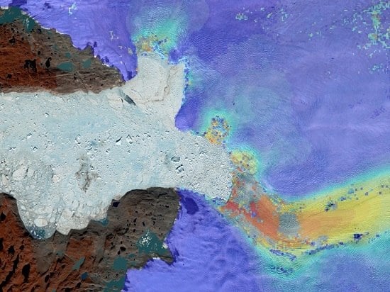
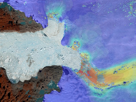
4.3. Greenland

Figure 15 shows ice velocity for the region around Jacobshavn Glacier (Sermeq Kujalleq), west coast of Greenland, using Sentinel-2A data sets of a 23-day interval (16 August–8 September 2015). We removed the overall co-location error derived from stable ground by applying a constant offset of 2.1 m and −3.0 m in North and East direction (Figure 10 and Figure 15b), which corresponds to a velocity of 0.09 m/day and −0.13 m/day for the time interval used.

Ice velocity is estimated by offset tracking with a filter window size of 72 × 72 pixels. Despite the time interval of 23 days and melting conditions on the outlet glaciers and the percolation zone of the ice sheet, the matching procedure detected sufficient features like crevasses for generating an almost complete ice velocity field. Some gaps of the ice velocity maps are found in the upper part of the percolation zone and on the terminus of the Jakobshavn Glacier with very high velocities of more than 30 m/d, which requires shorter time periods when surface features are better preserved. In addition, ice flows in a curve which leads to rotation of the features tracked and thus to lack of correlation when matching is based on image translation only [35].

We compared the Sentinel-2A ice velocity map with the Greenland mean ice velocity mosaic of 2015 derived from Sentinel-1A Interferometric Wide Swath data [36]. Figure 16 shows velocity profiles along the central flow line for the two outlet glaciers Sermeq Kujalleq (profile 1) and Sermeq Avannarleq (profile 2). Good agreement is seen between the velocities from Sentinel-2A and the mean Sentinel-1A based ice velocity map. This agreement suggests the possibility of a synergistic use of optical Sentinel-2 and SAR based Sentinel-1 velocity maps for generation of an ice sheet wide velocity map and for monitoring short-term temporal variation in ice speed using data from both sensors. At the lowermost part of the profiles shown, differences between the Sentinel-2 summer speeds and the Sentinel-1 mean annual speeds are clearly visible. To what extent the other smaller differences between the profiles are statistically significant is difficult to conclude at this point because (a) the Sentinel-1 profile is an annual average and the Sentinel-2 one refers to a specific period; and (b) because the accuracy of Sentinel-2 matches over the Greenland ice sheet could not be assessed yet.

4.4. Antarctic Peninsula

As a final test different from the mountain glaciers investigated above (Section 4.1 and Section 4.2), we examine Sentinel-2A derived ice displacements over a section of the Antarctic Peninsula, containing ice plateaus, outlet glaciers, calving glaciers, and parts of the Larsen C ice shelf. Based on Sentinel-2A band 8 images from 8 and 18 January 2016, we obtain maximum speeds of around 6 m/d (Figure 17). Also displacements on sea ice can be resolved (middle left edge of the section, around 2,560,000/600,000). The glaciers and parts of the Larsen C ice shelf with surface speeds on the order of 1 m/d (i.e., movements of one Sentinel-2 band 8 pixel and less) are well visible (see also [37]).

We find three types of conditions where the offset tracking failed, as expressed for instance by low correlation values that were then masked out in Figure 17: (i) clouds, as indicated in Figure 17. Near-surface clouds/fog to the lower right corner (around 700,000/2,500,000) in the 18 January 2016 image section were not detected by our simple automated cloud detection, i.e., not displayed as white areas in Figure 17, and thus corrupted displacement measurements. (Note: the default cloud mask that comes with the Sentinel-2 L1C data [38] fails in our example and marks most glacier areas outside of the ice shelf falsely as clouds); (ii) Correlation failed on parts of the plateau due to lack of coherent visual contrast; (iii) On large parts of the ice shelf, a matching window size of 40 × 40 pixels (400 m × 400 m) is too small with respect to the typical size of visual features to enable unique identification of corresponding features. In fact, window sizes of 2 km × 2 km reveal better results (small rectangular sub-panel in Figure 17), and larger windows even better ones (cf. [37]).

The results of Figure 17 were obtained after co-registering the two images over rock outcrops and removing a co-location offset of around −7 m in Easting and 8 m in Northing. Only at a few places are biases as described in Section 3.1 visible; stripes in the along-track direction can be seen at around 2,570,000/660,000 and 2,590,000/620,000 in Figure 17. This confirms the high potential of repeat-orbit Sentinel-2 data for precise ice-velocity measurements even over short time intervals. Biases between the swaths of individual pushbroom modules become visible, and might have to be observed or corrected in special cases, but will in general not have a major impact on ice displacements measured from Sentinel-2 data.

5. Conclusions

In this contribution, we analyse the radiometric and geometric performance of Sentinel-2A data with focus on glaciological applications, and evaluate the potential of repeat Sentinel-2 data for measuring glacier flow. Our studies are mainly based on ramp-up phase data, but also on some commissioning phase data.

For dark surfaces, we find along-track stripes of one pixel in width and an amplitude on the order of a few digital numbers, or a few 0.0001 TOA reflectance, presumably from the precision of destriping/radiometric calibration. Such biases will typically have negligible effect on automated ice/snow mapping. On brighter surfaces, only radiometric differences between the 12 pushbroom modules forming the Sentinel-2A focal plane may appear, with steps of up to a few tens of digital numbers. Also these offsets should typically not affect ice and snow mapping, but might become visible in some segmentation or classification products. The high dynamic range and radiometric resolution of Sentinel-2A are of great benefit for snow and ice studies [39].

Overall lateral offsets between Sentinel-2A L1C data from repeat orbits are typically on the order of 10 m or below, i.e., equal or smaller than the pixel size of the Sentinel-2 10 m bands. These values might improve in the future with co-registration of the data to a reference data set. Within L1C data from repeat orbits, lateral offsets of 1–2 m become visible in parts between the swaths of the individual 12 pushbroom modules.

In contrast to the small offsets between repeat-orbit data, lateral offsets between Sentinel-2A data from different orbits, or between Sentinel-2A and other data, such as Landsat, are strongly affected by vertical misrepresentations of the DEM used for ortho-rectification of the data (and also used for focusing of the different bands and pushbroom modules) that propagate mainly into cross-track offsets. In the worst case, a DEM error of 1 unit leads to a cross-track offset between two scenes of about 1/3 unit. In practice such offsets can amount to several 10-m pixels in size, especially over thinning glaciers. In relation to existing georeferenced information, these effects become smaller as they do not sum up from two scenes, but may still reach several pixels. The impacts from these propagated DEM errors range from comparably small problems over flat areas within the SRTM DEM cover, to SRTM cover in mountains with typical InSAR problems, and to areas outside the SRTM cover with potentially large DEM errors. In northern Norway for instance, locally varying cross-track offsets of 30–50 m between Sentinel-2A L1C (or between Sentinel-2 and Landsat) data from different orbits seem not uncommon, and we expect similar values for other mountainous areas outside the SRTM cover.

Such values of >1 pixel for lateral offsets become actually typical over glaciers, both within and outside SRTM coverage, as DEMs are almost by necessity outdated over glaciers with respect to the date of image acquisition. In the case of SRTM (acquisition in February 2000), >15 years of glacier thickness change, mostly loss, come into effect. For reference, glacier elevation losses of 5 m/year and more are not untypical for glacier tongues in the European Alps [22,40]. As a result, tracking ice velocities between repeat Sentinel-2 data from different orbits, or between Sentinel-2 and Landsat data becomes often problematic for small displacements of a few pixels or less. In order to keep the relative velocity errors small, glacier tracking using images from different orbits should be applied only for ice displacements that are one or several orders of magnitude larger than the cross-track offsets due to DEM errors expected over the glacier studied.

For repeat-orbit Sentinel-2A data, however, we find an impressive potential for ice flow measurements. The good radiometric and geometric performance of Sentinel-2 allows quantification of seasonal ice velocities even over 10-day cycles. We demonstrate this potential for Aletsch Glacier (Swiss Alps), Fox Glacier (New Zealand Alps), Jacobshavn Glacier and neighbouring outlet glaciers of the Western Greenland Icesheet, and a section of the Antarctic Peninsula close to the Larsen C ice shelf. The launch of Sentinel-2B and with that the availability of five-day repeat orbits will even further increase this potential, at least by reducing the probability of cloud cover. By triangulating displacement measurements between three subsequent acquisitions we show that ice velocities can be measured at least with an accuracy of 10%–20% of a 10-m pixel (i.e., 1–2 m). This creates a number of new possibilities for investigating glacier flow, its spatiotemporal variations, and terrain deformations in general.

References

- Paul, F.; Bolch, T.; Kääb, A.; Nagler, T.; Nuth, C.; Scharrer, K.; Shepherd, A.; Strozzi, T.; Ticconi, F.; Bhambri, R.; et al. The glaciers climate change initiative: Methods for creating glacier area, elevation change and velocity products. Remote Sens. Environ. 2015, 162, 408–426. [Google Scholar] [CrossRef]
- Roy, D.P.; Wulder, M.A.; Loveland, T.R.; Woodcock, C.E.; Allen, R.G.; Anderson, M.C.; Helder, D.; Irons, J.R.; Johnson, D.M.; Kennedy, R.; et al. Landsat-8: Science and product vision for terrestrial global change research. Remote Sens. Environ. 2014, 145, 154–172. [Google Scholar] [CrossRef]
- Drusch, M.; del Bello, U.; Carlier, S.; Colin, O.; Fernandez, V.; Gascon, F.; Hoersch, B.; Isola, C.; Laberinti, P.; Martimort, P.; et al. Sentinel-2: ESA’s optical high-resolution mission for GMES operational services. Remote Sens. Environ. 2012, 120, 25–36. [Google Scholar] [CrossRef]
- Gascon, F.; Cadau, E.; Colin, O.; Hoersch, B.; Isola, C.; Fernandeza, B.L.; Martimort, P. Copernicus Sentinel-2 mission: Products, algorithms and cal/val. Earth Obs. Syst. XIX 2014. [Google Scholar] [CrossRef]
- Winsvold, S.H.; Andreassen, L.M.; Kienholz, C. Glacier area and length changes in Norway from repeat inventories. Cryosphere 2014, 8, 1885–1903. [Google Scholar] [CrossRef]
- Paul, F.; Barrand, N.E.; Baumann, S.; Berthier, E.; Bolch, T.; Casey, K.; Frey, H.; Joshi, S.P.; Konovalov, V.; le Bris, R.; et al. On the accuracy of glacier outlines derived from remote-sensing data. Ann. Glaciol. 2013, 54, 171–182. [Google Scholar] [CrossRef] [Green Version]
- Winsvold, S.H.; Kääb, A.; Nuth, C. Regional glacier mapping using optical satellite data time series. IEEE J. Sel. Top. Appl. Earth Obs. Remote Sens. 2016. [Google Scholar] [CrossRef]
- Kääb, A.; Lamare, M.; Abrams, M. River ice flux and water velocities along a 600 km-long reach of Lena River, Siberia, from Satellite Stereo. Hydrol. Earth Syst. Sci. 2013, 17, 4671–4683. [Google Scholar] [CrossRef]
- Nuth, C.; Kääb, A. Co-registration and bias corrections of satellite elevation data sets for quantifying glacier thickness change. Cryosphere 2011, 5, 271–290. [Google Scholar] [CrossRef]
- Paul, F.; Winsvold, S.H.; Kääb, A.; Nagler, T. Glacier remote sensing using Sentinel-2. Part II: Mapping glacier extents and surface facies, and comparison to Landsat-8. Remote Sens. 2016, 8, 575. [Google Scholar] [CrossRef]
- Tucker, C.J.; Grant, D.M.; Dykstra, J.D. NASA‘s global orthorectified Landsat data set. Photogramm. Eng. Remote Sens. 2004, 70, 313–322. [Google Scholar] [CrossRef]
- Sun, G.; Ranson, K.J.; Khairuk, V.I.; Kovacs, K. Validation of surface height from shuttle radar topography mission using shuttle laser altimeter. Remote Sens. Environ. 2003, 88, 401–411. [Google Scholar] [CrossRef]
- Fahnestock, M.; Scambos, T.; Moon, T.; Gardner, A.; Haran, T.; Klinger, M. Rapid large-area mapping of ice flow using Landsat 8. Remote Sens. Environ. 2015. [Google Scholar] [CrossRef]
- Kääb, A.; Vollmer, M. Surface geometry, thickness changes and flow fields on creeping mountain permafrost: Automatic extraction by digital image analysis. Permafr. Periglac. Process. 2000, 11, 315–326. [Google Scholar] [CrossRef]
- Heid, T.; Kääb, A. Evaluation of existing image matching methods for deriving glacier surface displacements globally from optical satellite imagery. Remote Sens. Environ. 2012, 118, 339–355. [Google Scholar] [CrossRef]
- Kääb, A. Correlation Image Analysis Software (CIAS). 2013. Available online: http://www.mn.uio.no/icemass (accessed on 4 July 2016).
- Wang, R.; Muller, J.P.; Hu, C.; Zeng, T. Comparison between SRTM-C DEM and ICESat elevation data in the arid Kufrah area. In Proceedings of the IET International Radar Conference, Hangzhou, China, 14–16 October 2015; pp. 1–4. [CrossRef]
- Necsoiu, M.; Leprince, S.; Hooper, D.M.; Dinwiddie, C.L.; McGinnis, R.N.; Walter, G.R. Monitoring migration rates of an active subarctic dune field using optical imagery. Remote Sens. Environ. 2009, 113, 2441–2447. [Google Scholar] [CrossRef]
- Hermas, E.; Leprince, S.; Abou El-Magd, I. Retrieving sand dune movements using sub-pixel correlation of multi-temporal optical remote sensing imagery, northwest Sinai Peninsula, Egypt. Remote Sens. Environ. 2012, 121, 51–60. [Google Scholar] [CrossRef]
- Pfeffer, W.T.; Arendt, A.A.; Bliss, A.; Bolch, T.; Cogley, J.G.; Gardner, A.S.; Hagen, J.O.; Hock, R.; Kaser, G.; Kienholz, C.; et al. The Randolph glacier inventory: A globally complete inventory of glaciers. J. Glaciol. 2014, 60, 537–552. [Google Scholar] [CrossRef] [Green Version]
- Howat, I.M.; Negrete, A.; Smith, B.E. The Greenland ice mapping project (GIMP) land classification and surface elevation data sets. Cryosphere 2014, 8, 1509–1518. [Google Scholar] [CrossRef]
- Joerg, P.C.; Morsdorf, F.; Zemp, M. Uncertainty assessment of multi-temporal airborne laser scanning data: A case study on an alpine glacier. Remote Sens. Environ. 2012, 127, 118–129. [Google Scholar] [CrossRef] [Green Version]
- Dunse, T.; Schellenberger, T.; Hagen, J.O.; Kääb, A.; Schuler, T.V.; Reijmer, C.H. Glacier-surge mechanisms promoted by a hydro-thermodynamic feedback to summer melt. Cryosphere 2015, 9, 197–215. [Google Scholar] [CrossRef]
- Kääb, A.; Huggel, C.; Fischer, L.; Guex, S.; Paul, F.; Roer, I.; Salzmann, N.; Schlaefli, S.; Schmutz, K.; Schneider, D.; et al. Remote sensing of glacier- and permafrost-related hazards in high mountains: An overview. Nat. Hazards Earth Syst. 2005, 5, 527–554. [Google Scholar] [CrossRef]
- Heid, T.; Kääb, A. Repeat optical satellite images reveal widespread and long term decrease in land-terminating glacier speeds. Cryosphere 2012, 6, 467–478. [Google Scholar] [CrossRef]
- Debella-Gilo, M.; Kääb, A. Sub-pixel precision image matching for measuring surface displacements on mass movements using normalized cross-correlation. Remote Sens. Environ. 2011, 115, 130–142. [Google Scholar] [CrossRef]
- Redpath, T.A.N.; Sirguey, P.; Fitzsimons, S.J.; Kääb, A. Accuracy assessment for mapping glacier flow velocity and detecting flow dynamics from ASTER satellite imagery: Tasman Glacier, New Zealand. Remote Sens. Environ. 2013, 133, 90–101. [Google Scholar] [CrossRef]
- Ahn, Y.; Howat, I.M. Efficient automated glacier surface velocity measurement from repeat images using multi-image/multichip and null exclusion feature tracking. IEEE Trans. Geosci. Remote Sens. 2011, 49, 2838–2846. [Google Scholar]
- Schubert, A.; Faes, A.; Kääb, A.; Meier, E. Glacier surface velocity estimation using repeat TerraSAR-X images: Wavelet- vs. correlation-based image matching. ISPRS J. Photogramm. 2013, 82, 49–62. [Google Scholar] [CrossRef]
- Prats, P.; Scheiber, R.; Reigber, A.; Andres, C.; Horn, R. Estimation of the surface velocity field of the Aletsch glacier using multi-baseline airborne SAR interferometry. IEEE Trans. Geosci. Remote Sens. 2009, 47, 419–430. [Google Scholar] [CrossRef]
- Wang, D.; Kääb, A. Modeling glacier elevation change from DEM time series. Remote Sens. 2015, 7, 10117–10142. [Google Scholar] [CrossRef]
- Herman, F.; Anderson, B.; Leprince, S. Mountain glacier velocity variation during a retreat/advance cycle quantified using sub-pixel analysis of ASTER images. J. Glaciol. 2011, 57, 197–207. [Google Scholar] [CrossRef]
- Gjermundsen, E.F.; Mathieu, R.; Kääb, A.; Chinn, T.; Fitzharris, B.; Hagen, J.O. Assessment of multispectral glacier mapping methods and derivation of glacier area changes, 1978–2002, in the central southern alps, New Zealand, from ASTER satellite data, field survey and existing inventory data. J. Glaciol. 2011, 57, 667–683. [Google Scholar] [CrossRef]
- Purdie, H.L.; Brook, M.S.; Fuller, I.C.; Appleby, J. Seasonal variability in velocity and ablation of Te Moeka o Tuawe/Fox Glacier, South Westland, New Zealand. N. Z. Geogr. 2008, 64, 5–19. [Google Scholar] [CrossRef]
- Debella-Gilo, M.; Kääb, A. Measurement of surface displacement and deformation of mass movements using least squares matching of repeat high resolution satellite and aerial images. Remote Sens. 2012, 4, 43–67. [Google Scholar] [CrossRef]
- Nagler, T.; Rott, H.; Hetzenecker, M.; Wuite, J.; Potin, P. The Sentinel-1 mission: New opportunities for ice sheet observations. Remote Sens. 2015, 7, 9371–9389. [Google Scholar] [CrossRef]
- Haug, T.; Kääb, A.; Skvarca, P. Monitoring ice shelf velocities from repeat MODIS and Landsat data—A method study on the Larsen C ice shelf, Antarctic peninsula, and 10 other ice shelves around Antarctica. Cryosphere 2010, 4, 161–178. [Google Scholar] [CrossRef]
- Sentinel-2 Level-1C Land/Water and Cloud Masks. Sentinel Online—Technical Guides—Sentinel-2 MSI—Products and Algorithms—Level-1C Processing. Available online: https://sentinel.esa.int/web/sentinel/technical-guides/sentinel-2-msi/level-1c/land-water-cloud-masks (accessed on 10 June 2016).
- Pope, A.; Rees, W.G. Impact of spatial, spectral, and radiometric properties of multispectral imagers on glacier surface classification. Remote Sens. Environ. 2014, 141, 1–13. [Google Scholar] [CrossRef]
- Paul, F.; Haeberli, W. Spatial variability of glacier elevation changes in the Swiss Alps obtained from two digital elevation models. Geophys. Res. Lett. 2008, 35, L21502. [Google Scholar] [CrossRef]
© 2016 by the authors; licensee MDPI, Basel, Switzerland. This article is an open access article distributed under the terms and conditions of the Creative Commons Attribution (CC-BY) license (http://creativecommons.org/licenses/by/4.0/).
Share and Cite
Kääb, A.; Winsvold, S.H.; Altena, B.; Nuth, C.; Nagler, T.; Wuite, J. Glacier Remote Sensing Using Sentinel-2. Part I: Radiometric and Geometric Performance, and Application to Ice Velocity. Remote Sens. 2016, 8, 598. https://0-doi-org.brum.beds.ac.uk/10.3390/rs8070598
Kääb A, Winsvold SH, Altena B, Nuth C, Nagler T, Wuite J. Glacier Remote Sensing Using Sentinel-2. Part I: Radiometric and Geometric Performance, and Application to Ice Velocity. Remote Sensing. 2016; 8(7):598. https://0-doi-org.brum.beds.ac.uk/10.3390/rs8070598
Chicago/Turabian StyleKääb, Andreas, Solveig H. Winsvold, Bas Altena, Christopher Nuth, Thomas Nagler, and Jan Wuite. 2016. "Glacier Remote Sensing Using Sentinel-2. Part I: Radiometric and Geometric Performance, and Application to Ice Velocity" Remote Sensing 8, no. 7: 598. https://0-doi-org.brum.beds.ac.uk/10.3390/rs8070598