Article

Best Accuracy Land Use/Land Cover (LULC) Classification to Derive Crop Types Using Multitemporal, Multisensor, and Multi-Polarization SAR Satellite Images

1
Institute of Geography, University of Cologne, Albertus-Magnus-Platz, 50923 Cologne, Germany
2
Airbus Defence and Space, 88039 Friedrichshafen, Germany
3
Department of Plant Nutrition, China Agricultural University, Yuanmingyuan West Road No. 2, 100193 Beijing, China
*
Author to whom correspondence should be addressed.
Submission received: 15 March 2016 / Revised: 6 July 2016 / Accepted: 13 August 2016 / Published: 20 August 2016

Abstract

:
When using microwave remote sensing for land use/land cover (LULC) classifications, there are a wide variety of imaging parameters to choose from, such as wavelength, imaging mode, incidence angle, spatial resolution, and coverage. There is still a need for further study of the combination, comparison, and quantification of the potential of multiple diverse radar images for LULC classifications. Our study site, the Qixing farm in Heilongjiang province, China, is especially suitable to demonstrate this. As in most rice growing regions, there is a high cloud cover during the growing season, making LULC from optical images unreliable. From the study year 2009, we obtained nine TerraSAR-X, two Radarsat-2, one Envisat-ASAR, and an optical FORMOSAT-2 image, which is mainly used for comparison, but also for a combination. To evaluate the potential of the input images and derive LULC with the highest possible precision, two classifiers were used: the well-established Maximum Likelihood classifier, which was optimized to find those input bands, yielding the highest precision, and the random forest classifier. The resulting highly accurate LULC-maps for the whole farm with a spatial resolution as high as 8 m demonstrate the beneficial use of a combination of x- and c-band microwave data, the potential of multitemporal very high resolution multi-polarization TerraSAR-X data, and the profitable integration and comparison of microwave and optical remote sensing images for LULC classifications.

Graphical Abstract

1. Introduction

Satellite remote sensing is used as a powerful tool to monitor the Earth’s surface, particularly in producing land use and land cover (LULC) classifications [1,2]. In general, creating LULC classifications builds upon two imaging methods: optical and microwave remote sensing. Both sensing approaches imply distinct advantages and disadvantages. While optical sensors rely on reflectance and cloud free conditions, microwave sensors only capture the backscatter in a given wavelength [3]. Examples of optical LULC analysis on a global scale are given by Chen et al. [4], for example, and for a regional scale by Lo and Fung [5], and Immitzer et al. [6]. Microwave imaging using synthetic aperture radar (SAR) images for LULC emerged in the 1980s, and examples are described by Bryan [7] and Dobson et al. [8]. The combined analysis of optical and microwave imagery to use the advantages of both systems for LULC classifications was investigated by Solberg et al. [9], McNairn et al. [10], Forkuor et al. [11], and Blaes et al. [12].
A common information gap in LULC classifications and products are detailed crop classes within the arable land use class [13]. For numerous agricultural applications, the spatial information of arable land is not sufficient. This is true for agro ecosystem modeling [14], yield estimation [15], subsidy control [16], and retrieval of biophysical plant parameters on regional scales [17]. However, using satellite remote sensing to differentiate crops is a demanding task, as different crop types have similar reflection properties in remote sensing images for some periods of the year [18]. Those crops can only be separated from each other by a multitemporal analysis, which considers the phenology of the investigated crops [3]. Multitemporal and multispectral optical and infrared remote sensing has proved to be an effective approach to discriminate different crops [19]. However, as mentioned above, the availability of optical satellite-borne imagery is sometimes limited due to cloud cover in the region of interest. Therefore, for many agricultural regions it is a coincidence whether optical images from the right time are available or not, which makes crop classifications based on optical imagery unreliable.
The key advantage of satellite-borne SAR imaging is the independence from cloud cover, and as it is an active sensing system, also from sun-induced reflection. Consequently, SAR imagery has become an important tool to distinguish agricultural crops [12,20,21,22,23]. Sophisticated SAR systems provide a temporal resolution that lies within a few days, with a spatial resolution as high as 20 cm [24]. Such systems are already in application to deliver annual crop inventories on regional levels [10]. Recently, polarimetric SAR images have been analysed using decomposition theorems such as the alpha/entropy decomposition [25], which increases the accuracy of LULC analysis from microwave data. Especially in rice-growing regions (which usually have a very high cloud cover during the growing season), polarimetric SAR has been intensively used as a monitoring tool [26,27,28,29,30,31].
However, there is a wide choice of different remote sensing satellites, radar, and optical. While optical satellites usually operate in one imaging mode, radar satellites can be programmed to work in different configurations. The user has to choose the polarization configuration, the incidence angle, and the spatial resolution as a result of the chosen imaging mode [32]. Interestingly, only a few studies such as McNairn et al. [23] deal with multisensor data (i.e., the combination and comparison of SAR images from more than one satellite). Furthermore, to the knowledge of the authors, no other studies investigate the comparison of different imaging modes from the same sensor in the context of crop classification. In addition, the image information gained from optical and microwave sensing methods contains different LULC properties. Consequently, combined approaches of using optical and microwave images can improve the LULC analysis [9,10,11,12].
For a LULC analysis, an extensive set of ground truth is typically mapped and separated into two datasets. One dataset is used to train the classifier for the automated classification of the entire image. The second dataset is used to evaluate the classification’s accuracy. Results of the evaluation are summarized in a confusion matrix [1]. Based on the confusion matrix, statistical accuracy parameters are calculated. One is the overall accuracy [33], which counts pixels that are correctly classified in the reference divided by all pixels that are taken for reference. This procedure applies for both optical and microwave image classification.
Considering the need for multitemporal and multisensor radar image classification in a combined approach with optical image analysis for crop classification, this study is framed by three objectives. (i) To investigate how to derive LULC classifications from multitemporal, multisensor, and multi-polarisation SAR satellite images with the best possible accuracy; (ii) to evaluate the potential of those images and the combinations to obtain a crop type map with a spatial resolution as high as 8 m; (iii) to identify the best combination of available input images that yields the best classification accuracy for each respective part of the study area.

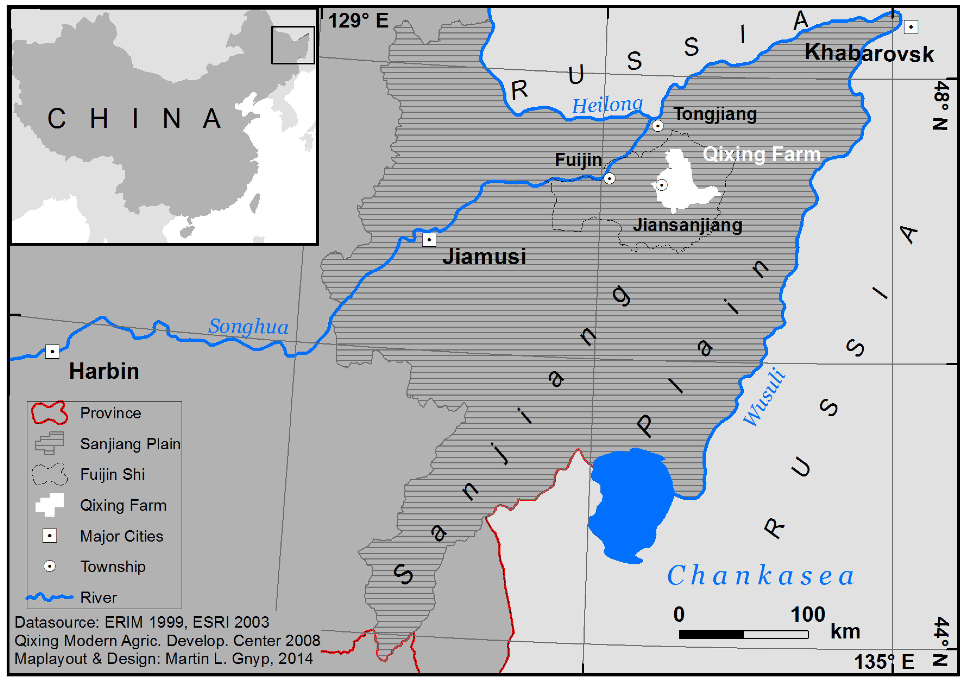
2. Study Area and Data

The study area is the Qixing farm, situated in northeast China, in the Sanjiang Plain (Figure 1). The climate is continental and influenced by monsoonal effects. As a result, the area is characterized by a cold and dry winter and a relatively warm summer with sufficient precipitation for high-yield agriculture [35]. The growing season is short and lasts for about five months. Thus, only one yield per year is possible. Main crops include: paddy-rice, summer-wheat, soya-beans, pumpkins, and maize. Additionally, the terrain of the whole farm is virtually flat.
During the 2009 growing season, between June and October, we collected ground data of field crop distribution. A total of 22 agricultural fields, 3 areas of rural villages, and one lake, covering an area of about 5 km2 were investigated several times. Based on the observations, their spatial extents were transferred to a Geographic Information System (GIS). Table 1 shows the spatial statistics of the dataset. The collection of fields was equally divided into a training dataset and an independent validation dataset. Different fields were either used for training or validation. Unfortunately, only one pumpkin field, one lake, and one deciduous forest were situated in the area of interest. In those cases, we divided single areas into two parts and used one part for training and the other for validation. All observed fields lie in an area covered by all remote sensing images. Furthermore, the area of the validation was roughly matched to be representative of the study area.
As described in Section 1, optical satellite images can be used exclusively under cloud-free conditions in the area of interest. In the year of investigation, we observed unusually long periods of rainy and cloudy weather. The consequence was that only the FORMOSAT-2 image from the beginning of August had a low enough cloud cover over the area where the training and validation field data were collected. Various other optical images could not be used because of too many clouds in the images.
Since SAR imaging is not influenced by clouds and haze in the atmosphere, all 12 microwave images obtained during the growing season of 2009 could be used for this study. Acquisition numbers 1–4 (Table 2) are a time series of very high resolution TerraSAR-X images in dual polarization. A second time series consists of images 5–8 (Table 2), which were taken in stripmap mode with only one polarization and have a lower spatial resolution. While the data density of this time-series is generally lower, the covered area is about 20 times larger, but still does not cover the whole area of the farm. Dataset 10–13 (Table 2) are from the Radarsat-2 and Envisat satellites. They operate in c-band, which means increased wavelength and therefore sensitivity to other properties of the ground. While they have a lower spatial resolution, more area is imaged at once. Indeed, the Envisat image is the only one covering the whole area of the farm. The polarizations of the Radarsat-2 acquisitions are horizontal-send–horizontal-receive (HH) and horizontal-send—vertical receive (HV). For the Envisat acquisition, the polarization configuration is the same, but the directions of the polarizations are inverted (VV and VH).

3. Methods

As described in Section 2, the remote sensing data differ from each other in one basic aspect: The TerraSAR-X Spotlight data (dataset no. 1–4, Table 2) and the cloud-free part of the FORMOSAT-2 image only cover the area where the ground data are taken. The TerraSAR-X stripmap data (datasets no. 5–9,Table 2), the Radarsat-2, and Envisat data cover a much wider area, but with a decreased spatial resolution. Therefore, we divided our data into two subsets. One contains the data that cover a small area at a very high resolution (dataset no. 1–4, 13). The other subset contains images no. 5–12 (Table 2), and is used to provide land use information for the whole Qixing farm, which covers an area of about 1070 km2.
To process the remote sensing images, the following software packages were used: The polarimetric radar images were processed with Polsarpro. The European Space Agency (ESA) provided the Next ESA SAR Toolbox (NEST) (new name: SNAP/ Sentinel-1 Toolbox), which was used for speckle filtering and range doppler terrain correction. For the co-registration of the FORMOSAT-2 image, we used ENVI 5.0. The Maximum Likelihood classification and its optimization (Section 3.4) and the error assessment was done using ArcGIS 10.1 and the python scripting extension. The python script can be downloaded freely using the associated enrichments. The implementation of the Random Forest Classifier (Section 3.5) was done using the statistics software R [36] (Version 3.2.5) and the randomForest package [37] (Version 4.6.12), with a script published by [38].

3.1. Retrieval of Polarimetric Features

The measured signal from coherent polarimetric SAR systems can be analysed by determining the covariance matrix C and the coherency matrix T from the measured signal. The elements of those matrices can be directly used as input parameters in LULC classifications. As both matrices are related to each other, and [39] found out that the two matrices lead to similar classification results, we concentrated on the elements of the covariance matrix C. Furthermore, by eigenvector analysis of T it is possible to calculate entropy and alpha, which can be related to backscatter mechanisms on the ground. This is an advantage to single polarization systems and significantly improves the results of LULC classifications [40].
In this study, we obtained the possible parts of C from the dual polarimetric data from Radarsat-2 (datasets 9 and 10, Table 2) and TerraSAR-X (datasets 1–4, Table 2). In the case of the Radarsat-2 images, the cross elements of C (c12i, c12r) were excluded, because visual inspection revealed poor quality and unsuitability for LULC mapping. Additionally, based on the spatially averaged (5 × 5 window) coherency matrix T, we calculated the dual-pol entropy, alpha angle, and the degree of polarization [41]. In total, we derived seven individual rasters for each coherent TerraSAR-X polarimetric radar scene, and five for each Radarsat-2 scene.

3.2. Preprocessing of the Remote Sensing Data

For the Envisat ASAR image (dataset 12, Table 2), polarimetric decompositions as described in Section 3.1 is impossible, as the signal is not recorded coherently [42]. In this case, only the amplitudes of the radar signal were computed and used for the LULC classification. The same applies for the TerraSAR-X scenes that only contain one polarization (datasets 5–9, Table 2).
For all radar data, the next step was a multilooking, which decreases the pixel size, but reduces the speckle effect. Range and azimuth multilooking windows were chosen to roughly match the 8 m pixel size of the final classification.
The orthorectification of radar images is a transformation from slant range radar geometry to ground range, and involves the usage of a digital elevation model (DEM). We used data from the Shuttle Radar Topography Mission (SRTM) in 90 m resolution [43] to carry out a range-doppler terrain correction as described by Curlander and McDonough [44]. During this process, the final pixel size of 8 m was determined. We chose 8 m for all products in order to be able to compare and combine the images with the optical FORMOSAT-2 image on the pixel level. Furthermore, 8 m is a good compromise between oversampling the Radarsat-2 and Envisat ASAR data and undersampling of the TerraSAR-X data. Additionally, 8 m per pixel seems to be a decent size to determine fields in this region, as our field investigations have shown that they are rarely smaller than 20 m in diameter.
The orthorectification described above has to be carried out with high spatial precision for the intended pixel-based analysis. Therefore, it is worth looking at the anticipated positional error of the orthorectified radar images. It mainly depends on the location error of the position of the sensor platform during image acquisition and the error of the used DEM [44]. The first error is known to be low for TerraSAR-X [45], Radarsat-2 [46], and Envisat [47]. Concerning the second error, Rodriguez et al. [48] state the absolute error of the SRTM to be below 10 m. The resulting low positional error of the images is required for the combined pixel-based processing of the scenes. For a more detailed analysis of this aspect, see [17], where a subset of the same dataset was used to create a spatial reference for various other datasets.
In the next step, two speckle filters were applied to all images in the ground range to decrease the speckle effect. First, the gamma map filter with a with a 5 × 5 kernel size, and second, a rather simple median-filter with a kernel size of 3 × 3. More radar-specific image filters resulted in residuals in the final classification and tend to have a negative impact on the results.
In contrast, the optical FORMOSAT-2 image does not need such sophisticated preprocessing; it was co-registered to the orthorectified TerraSAR-X Spotlight images and thereby benefits from their high spatial accuracy. The RMSE (root mean square error) was 0.79 m, which is less than one pixel and allows a pixel-based combination of the image with the involved SAR images.

3.3. Supervised LULC Classification Using Remote Sensing Images

The training part of the ground reference data was used to carry out a supervised classification, during which a classifier assigns each pixel location to a certain land use class. The two different classifiers used in this study are the Maximum Likelihood classifier, in combination with a newly-developed optimization approach, further described in Section 3.4. The second is the Random Forest classifier, described in Section 3.5.
The different land use classes for forest and urban were not of interest for this study, and based on visual examination, it was clear that none of the remote sensing images would be able to discriminate between those classes. Consequently, after the classification, the deciduous and coniferous forest classes were merged into forest, while concrete was dissolved in urban.
The following validation process to quantify the accuracy of the LULC-classifications was based on independent ground reference. We chose overall accuracy as the most prominent measure of accuracy in this study. It is obtained by dividing all correctly classified pixels by all pixels that were used for validation [33,49]. Additionally, we calculated the confusion matrix (which allows more interpretation of the individual accuracy of the different land use classes) and the kappa-coefficient (κ), which illustrates accuracy compared to a random classification.

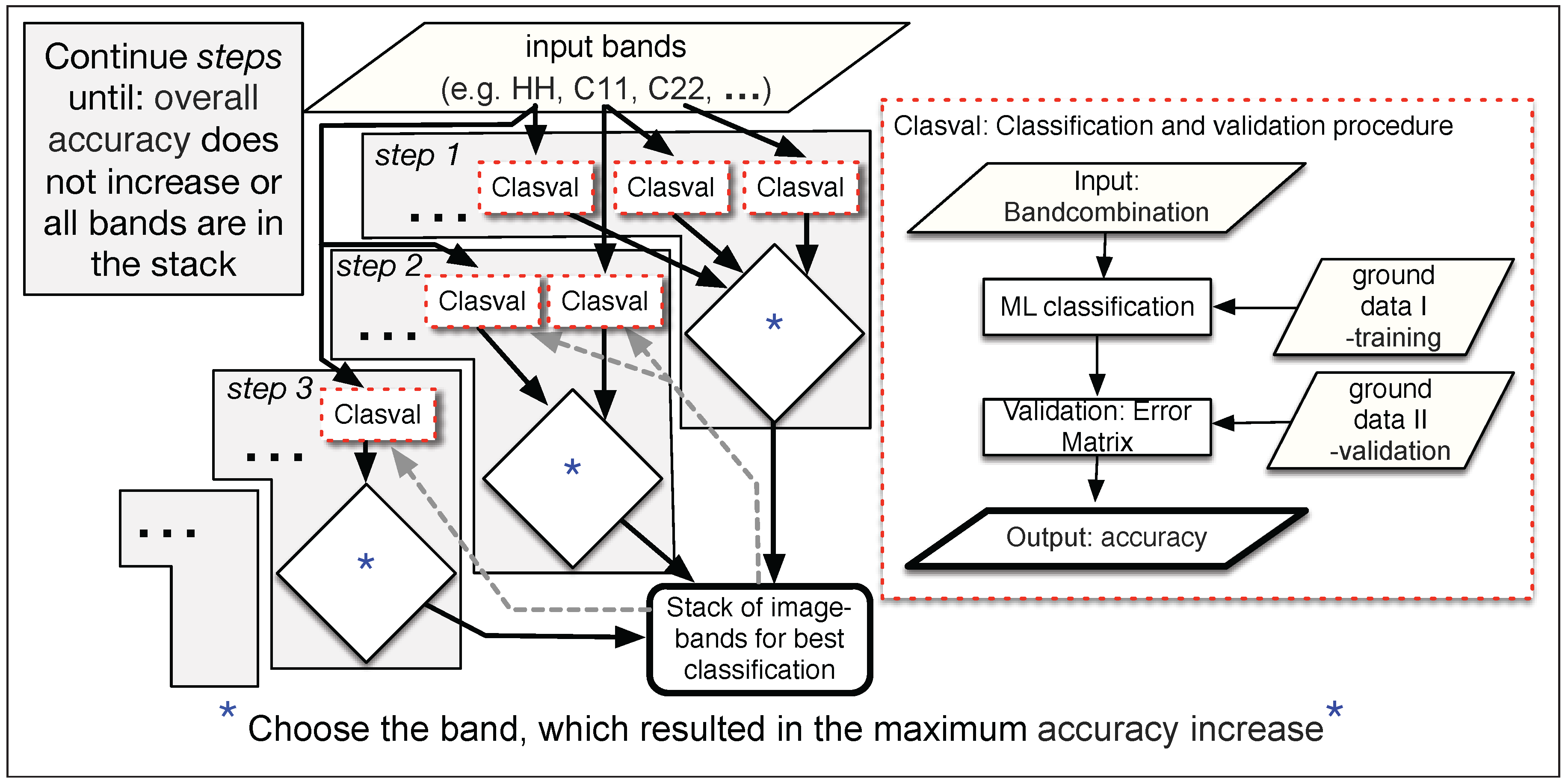
3.4. Maximum Likelihood Classification and Optimization

The supervised classification using the established Maximum Likelihood classifier was transformed to a python code using the scripting extension provided by ArcGIS. With this extension, it is possible to execute all software tools from a programming environment. Next, we implemented an innovative script logic to determine the raster band combination that results in the highest accuracy of the LULC classification, which likewise indicates that this band combination is suited best for the respective classification. Basically, the whole process was repetitively executed with stepwise addition of the input bands, until the highest accuracy was reached or all input bands were used. Figure 2 visually shows the workflow of the process. The script logic in pseudo-code is as follows:
  • Classify and validate all input raster bands individually.
  • Choose the one which results in the classification with the highest accuracy.
  • Combine this/these band(s) of the final stack successively with those bands that are not in the final stack. Add the band whose combination resulted in the highest accuracy-increase into the final stack.
  • Repeat step 3 until the accuracy does not increase any more or all bands are used.
In the end, this optimization process reveals those bands resulting in an increase of accuracy when added to the image stack of the classification. All other bands are neglected. Thereby, the optimum combination of input bands can be found, over-fitting is avoided, and erroneous information is dislodged. Furthermore, all input features are evaluated, whether they are able to increase the classification accuracy or not, which expresses the usefulness of this feature for the classification.

3.5. Random Forest Classification
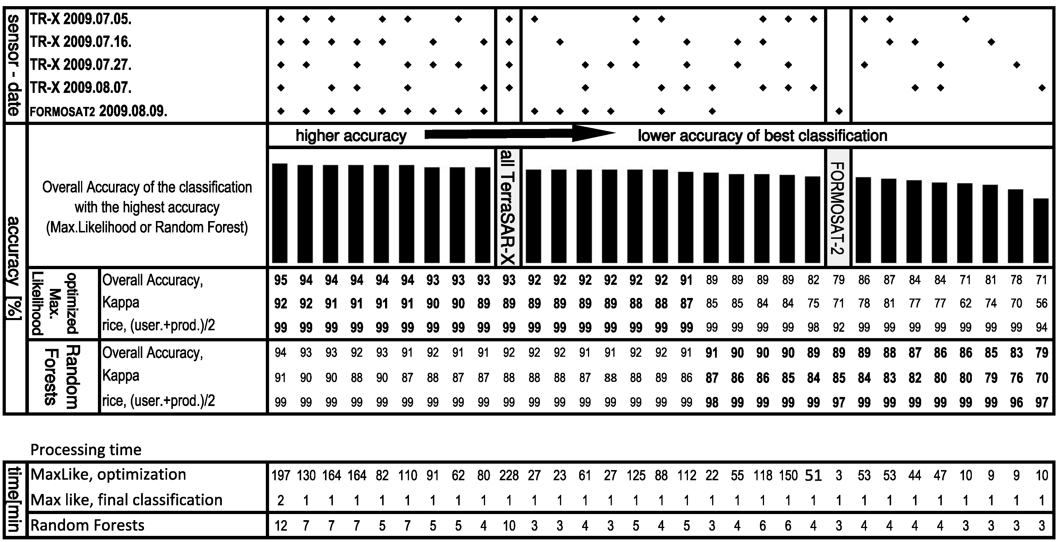
The second classifier implemented in this study is the Random Forest classification algorithm, introduced by Breiman [50] and adopted for the classification of remote sensing images by Pal [51]. Random Forest is a ensemble learning technique, and builds upon multiple decision trees. Each decision tree is built using a subset of the original training data and is evaluated by the remaining part of training features. New objects are classified as the class that is predicted by the most trees. According to [52], the classifier has three main advantages for LULC classifications from remote sensing images: (i) It reaches higher accuracies than other machine learning classifiers; (ii) It has the ability to measure the importance level of the input images; (iii) It does not make any assumptions about the distributions assumptions of the input images. Therefore, Random Forest classifications have been successfully applied to crop classification scenarios using remote sensing images, optical [53], and radar [54,55]. Ok et al. [56] concluded an accuracy increase using the Random Forest classifier over the Maximum Likelihood classifier of about eight percent to classify crops using one Spot5 satellite image.

4. Results

As described before, the input datasets were divided into spatial subsets. One consists of the scenes with a high resolution and the cloud-free part of the optical image. This area has a smaller extent of about 5 × 10 km. The resulting 31 combinations were each classified using the proposed optimized Maximum Likelihood approach and the Random Forest classifier. An overview of those results is given in Figure 3, whereas individual classifications are presented in Figure 4, Figure 5 and Figure 6. The second spatial subset consists of the five stripmap images of TerraSAR-X, the two Radarsat2 scenes, and the Envisat ASAR image. The 15 meaningful combinations of this subset were also each classified with both classifiers; results are shown in Figure 7. Additionally, the processing time of each of the 92 classifications is stated.
As an illustration, Figure 4 shows the result of the the combination of the four TerraSAR-X Spotlight images (datasets 1–4, Table 2), which results in an accuracy as high as 93%. By adding the optical FORMOSAT-2 image, it was possible to reach a higher accuracy of 95%—the highest accuracy of the study—which is shown in Figure 5 . When only two or three radar images are used, the accuracy declines. Notably, one Spotlight TerraSAR-X Radar acquisition alone still enables the determination of the rice cultivation area with minimum 97% when using Random Forest, and 94% with the Maximum Likelihood classifier. However, if two TerraSAR-X Spotlight acquisitions are combined, the overall accuracy reaches at least 86% (Random Forest). Especially of note, the rice accuracy becomes ideal (>99%). The rice accuracy of the classification of the optical image alone reaches 97%, whereas the accuracy of this classification is slightly higher than the classifications of each single radar acquisition. Interestingly, any combination of radar and optical images results in substantially increased accuracy indices. Nevertheless, the best combination of one single radar image (5 July 2009) and the optical FORMOSAT-2 image reaches an accuracy of 92% (κ-index of 0.89%), regardless of the classifier used, and is the one where the timespan between the acquisitions is longest. This result is shown in Figure 6. This smaller subset also demonstrates the benefit of the Optimization approach. On the one hand, once the optimum features are selected, the runtime is considerably reduced; on the other hand, an analysis of all selected features is possible, as shown in Table 3.
In comparison to the high accuracy values of the small subset, the classifications of the wider area exhibit lower classification accuracy. As can be seen, the area at the eastern end of the farm was classified with lower accuracy, as it was obtained from the Envisat image alone. Fortunately, only for about 8 km2 of the farm is this the only available source. Westwards, successively adding the two Radarsat-2 scenes increases the overall accuracy and the accuracy of the rice class to 89% (85% for Random Forest) after adding the first, and 0.96% (Random Forest and Maximum Likelihood) after also adding the second one. Notably, the combination of the two c-band images that are only one day apart from each other (datasets 10 and 12, Table 2) is the worst combination of the study. The two Radarsat-2 scenes are from different angles, and when classified alone, their accuracy is slightly higher than the one obtained from the five TerraSAR-X stripmap images (datasets 5–9, Table 2), which all have the same viewing geometry but only VV-polarization. In contrast, all combinations of the x-band time series with each c-band image yields a considerably higher accuracy. However, the best combination of images reaches 85% accuracy, which is still lower than the 89% that was obtained from the optical image. When it comes to the accuracy of the rice class, the combination is just able to outperform the optical image (98% vs. 97%). This radar combination covers 80% of the Qixing farm, which equals about 872 km2, and the major parts of Figure 8 contain this classification.

5. Discussion

Both the developed optimized Maximum Likelihood classification and the Random Forest classifier work well for LULC and crop analysis based on multitemporal, multisensor, and multi-polarization SAR satellite images. The analysis of four TerraSAR-X Spotlight images results in an accuracy of 93% and 92% for Maximum Likelihood and Random Forest, respectively, and of up to 99% for the rice crop class. The combined analysis of those four images with an optical FORMOSAT-2 image slightly improved the classification to a maximum of 95% overall accuracy (rice accuracy: 99%). Additionally, the mono-temporal analysis of the four TerraSAR-X Spotlight acquisitions are each able to determine the area of rice with a very high accuracy of at least 94%. This is not a new discovery, and is a consequence of the special interaction of microwaves with inundated rice fields [30,57]. By making use of this interaction, rice fields can be separated from the other land use classes with high accuracy [27,31,58]. Another known fact that can be justified by this study is that only multi-temporal radar acquisitions are adequate to dissolve different crops [20,21]. Bush and Ulaby [20] also used dual polarimetric SAR data and recommended four target revisits at an interval of ten days to get 90% accuracy. We can almost exactly conclude the same from our study, as the four TerraSAR-X acquisitions—which are 11 days apart from each other—resulted in accuracy of 93% and 92%, depending on the classifier. This is also in accordance with the more recent study of Bargiel and Herrmann [22], who reached about 90% accuracy using 14 TerraSAR-X images to separate different crops in two regions. However, in this study, the only way to further increase such high accuracies was the combination with the optical FORMOSAT-2 image, which delivered an accuracy of up to 95%. This justifies the studies of Blaes et al. [12] and Forkuor et al. [11]. Notably, our study additionally quantifies the benefit of the optical image: Its availability substitutes about two TerraSAR-X Spotlight images, as combinations of two radar images and the optical image deliver accuracies about as high as the four radar images combined.
These results of the small subset show how the developed approach is well-suited to reproduce and validate existing knowledge and quantify accuracy improvements from added remote sensing datasets. In the same way, Figure 7 shows accuracy for the wider area, which is influenced by different aspects. Again, accuracy generally increases when more data is added. Additionally, we demonstrated the beneficial use of combined x- and c-band radar images for crop classification, which has been shown before by McNairn et al. [23]. The wider area is also a good test-bed for the comparison of the two classifiers used in the study. The Random Forest classifier seems to be much more effective in data-poor situations; the worst classification from the single Envisat image alone is the extreme example—it has a 16% higher overall accuracy using Random Forest than the same classification using Maximum Likelihood. Interestingly, in data intensive environments of the study, the proposed optimization of the Maximum Likelihood is able to very slightly outperform the Random Forest classifier. Analysis of the processing time reveals the potential of the Maximum Likelihood classifier to be carried out much faster, once the optimal band combination is determined.
Although our findings offer some insights on crop classification using diverse SAR satellite images, the limitations of the study design and outcomes should be recognized. First of all, the crop types presented in this study are limited. It would be interesting to investigate the potential to classify other crops with even more diverse SAR images. Those could also be extended to fully polarimetric images, which offer much more possibilities to derive polarimetric features. Qi et al. [40], for instance, derived as many as 80 different features from two fully polarimetric Radarsat-2 acquisitions for their pixel-based approach. Furthermore, Souyris et al. [59] quantified the increase of accuracy from fully polarimetric versus dual polarimetric L-band images. Another issue with our study is that more possible SAR satellites and more SAR acquisition modes were not incorporated. Data from the L-band SAR sensor PalSAR onboard the ALOS satellite would extend our analysis to another wavelength, with an evaluation of its already-demonstrated crop classification potential [60] and the possibility to study the synergistic effects of l-, c- and x-band SAR data.
Another key point, especially for the small and more data-intense subset, is the question of whether or not that many radar datasets at such a high resolution are necessary. For instance, we described above that the accuracy of the rice class is always higher from SAR images. Notably, every high-resolution acquisition alone or any combination of two radar images is sufficient to differentiate the area of rice. Only when other classes are relevant and a high overall accuracy is needed, do more radar acquisitions actually make sense. The accuracy of the classification of the whole farm distinguishes the area of rice with more than 98% accuracy for 80% of the area of the farm, and the accuracy reaches 85 %. According to Anderson et al. [61], this is suitable for application.

6. Conclusions

In this study, we determined Land Use Land Cover of a rice farm in north-eastern China. The main objective was to fill the information gap of detailed crop classes within the arable land use class using a combination of multitemporal, multisensor, and multi-polarisation microwave satellite acquisitions. Forty-six different combinations of acquisitions were evaluated, and their accuracy quantified. A supervised classification was carried out using two different classifiers. The state-of-the-art Random Forest classifier and the well-established Maximum Likelihood classifier, which was optimized using an innovative script to find the optimum input bands. Finally, the classifications were merged to reach an optimized classification of the whole farm with the best accuracy possible. This final classification covers more than 1000 km2, in a spatial resolution as high as 8 m. Most of the area of the farm was classified with more than 85% accuracy, while the accuracy of the land cover class rice (which is the most important one) was almost perfect.
The results of the study concur with various studies on SAR-based crop classification. Furthermore, the potential of microwave and optical images to differentiate the area of rice is demonstrated and quantified on a regional scale with very high spatial resolution. It is shown that microwave and optical remote sensing is eminently suitable to discriminate the area of rice with high spatial resolution.
Data from c-band radar satellites such as Sentinel-1, Radarsat-2, and the future Radarsat constellation combined with operational x-band satellites such as TerraSAR-X, TanDEM-X, and PAZ make the presented approach ideal for even more data-intense study sites and years in the future. It is well suited to be adopted for other LULC crop distribution studies on regional scales. As the Maximum Likelihood optimization script is freely downloadable, all that is needed is therefore a ground truth set of crop distribution of the respective year and remote sensing images. The possibility to integrate multiple acquisitions from different sensors and automatically find the ideal combination of bands for land use classification is an important improvement for future LULC mapping from satellite remote sensing observations.

Supplementary Files

Supplementary File 1

Acknowledgments

This study was financially supported by National Basic Research Program (973-2015CB150405), International Bureau of the German Federal Ministry of Research and Technology BMBF (Project number CHN 08/051), Airbus Defence and Space, the GIS and RS group of the University of Cologne, the International Center for Agro-Informatics and Sustainable Development (ICASD), and the Sino-Norwegian Cooperative SINOGRAIN project (CHN-2152, 14-0039). Envisat ASAR Data were provided by the European Space Agency under proposal No. 16975 “Rice Monitoring China, Jiansanjiang”.

Author Contributions

Christoph Hütt conducted the field campaign, did the processing of the remote sensing scenes, wrote the python script for the automated classification approach, and the manuscript. Yuxin Miao supervised and managed the field work. Wolfgang Koppe planned and coordinated the TerraSAR-X acquisitions, and provided expertise on radar remote sensing. Georg Bareth provided expertise on remote sensing and land use classifications, and co-prepared the manuscript. Editorial contributions to the manuscript were made by Georg Bareth.

Conflicts of Interest

The authors declare no conflict of interest.

References

  1. Foody, G.M. Status of land cover classification accuracy assessment. Remote Sens. Environ. 2002, 80, 185–201. [Google Scholar] [CrossRef]
  2. Green, K.; Kempka, D.; Lackey, L. Using remote sensing to detect and monitor land-cover and land-use change. Photogramm. Eng. Remote Sens. 1994, 60, 331–337. [Google Scholar]
  3. Gomez-Chova, L.; Tuia, D.; Moser, G.; Camps-Valls, G. Multimodal classification of remote sensing images: A review and future directions. Proc. IEEE 2015, 103, 1560–1584. [Google Scholar] [CrossRef]
  4. Chen, J.; Chen, J.; Liao, A.; Cao, X.; Chen, L.; Chen, X.; He, C.; Han, G.; Peng, S.; Lu, M.; et al. Global land cover mapping at 30 m resolution: A POK-based operational approach. ISPRS J. Photogramm. Remote Sens. 2015, 103, 7–27. [Google Scholar] [CrossRef]
  5. Lo, C.P.; Fung, T. Production of land-use and land-cover maps of central Guangdong Province of China from LANDSAT MSS imagery. Int. J. Remote Sens. 1986, 7, 1051–1074. [Google Scholar] [CrossRef]
  6. Immitzer, M.; Vuolo, F.; Atzberger, C. First experience with Sentinel-2 data for crop and tree species classifications in Central Europe. Remote Sens. 2016, 8, 166. [Google Scholar] [CrossRef]
  7. Bryan, L.M. Urban land use classification using synthetic aperture radar. Int. J. Remote Sens. 1983, 4, 215–233. [Google Scholar] [CrossRef]
  8. Dobson, M.C.; Ulaby, F.T.; Pierce, L.E. Land-cover classification and estimation of terrain attributes using synthetic aperture radar. Remote Sens. Environ. 1995, 51, 199–214. [Google Scholar] [CrossRef]
  9. Solberg, A.H.S.; Jain, A.K.; Taxt, T. Multisource classification of remotely sensed data: Fusion of Landsat TM and SAR images. IEEE Trans. Geosci. Remote Sens. 1994, 32, 768–778. [Google Scholar] [CrossRef]
  10. McNairn, H.; Champagne, C.; Shang, J.; Holmstrom, D.; Reichert, G. Integration of optical and Synthetic Aperture Radar (SAR) imagery for delivering operational annual crop inventories. ISPRS J. Photogramm. Remote Sens. 2009, 64, 434–449. [Google Scholar] [CrossRef]
  11. Forkuor, G.; Conrad, C.; Thiel, M.; Ullmann, T.; Zoungrana, E. Integration of optical and Synthetic Aperture Radar imagery for improving crop mapping in Northwestern Benin, West Africa. Remote Sens. 2014, 6, 6472–6499. [Google Scholar] [CrossRef]
  12. Blaes, X.; Vanhalle, L.; Defourny, P. Efficiency of crop identification based on optical and SAR image time series. Remote Sens. Environ. 2005, 96, 352–365. [Google Scholar] [CrossRef]
  13. Atzberger, C. Advances in remote sensing of agriculture: Context description, existing operational monitoring systems and major information needs. Remote Sens. 2013, 5, 949–981. [Google Scholar] [CrossRef]
  14. Lenz-Wiedemann, V.I.S.; Klar, C.W.; Schneider, K. Development and test of a crop growth model for application within a Global Change decision support system. Ecol. Model. 2010, 221, 314–329. [Google Scholar] [CrossRef]
  15. Vibhute, A.D.; Gawali, B.W. Analysis and modeling of agricultural land use using remote sensing and geographic information system: A review. Int. J. Eng. Res. Appl. (IJERA) 2013, 3, 81–91. [Google Scholar]
  16. Schmedtmann, J.; Campagnolo, M.L. Reliable crop identification with satellite imagery in the context of common agriculture policy subsidy control. Remote Sens. 2015, 7, 9325–9346. [Google Scholar] [CrossRef]
  17. Zhao, Q.; Hütt, C.; Lenz-Wiedemann, V.I.S.; Miao, Y.; Yuan, F.; Zhang, F.; Bareth, G. Georeferencing multi-source geospatial data using multi-temporal TerraSAR-X imagery: A case study in Qixing farm, Northeast China. Photogramm. Fernerkund. Geoinf. 2015, 2015, 173–185. [Google Scholar] [CrossRef]
  18. Waldhoff, G.; Curdt, C.; Hoffmeister, D.; Bareth, G. Analysis of multitemporal and multisensor remote sensing data for crop rotation mapping. ISPRS Int. Arch. Photogramm. Remote Sens. Spat. Inf. Sci. 2012, I-7, 177–182. [Google Scholar] [CrossRef]
  19. Pinter, P.J., Jr.; Hatfield, J.L.; Schepers, J.S.; Barnes, E.M.; Moran, M.S.; Daughtry, C.S.; Upchurch, D.R. Remote sensing for crop management. Photogramm. Eng. Remote Sens. 2003, 69, 647–664. [Google Scholar] [CrossRef]
  20. Bush, T.; Ulaby, F. An evaluation of radar as a crop classifier. Remote Sens. Environ. 1978, 7, 15–36. [Google Scholar] [CrossRef]
  21. Hoogeboom, P. Classification of agricultural crops in radar images. IEEE Trans. Geosci. Remote Sens. 1983, GE-21, 329–336. [Google Scholar] [CrossRef]
  22. Bargiel, D.; Herrmann, S. Multi-temporal land-cover classification of agricultural areas in two European regions with high resolution spotlight TerraSAR-X data. Remote Sens. 2011, 3, 859–877. [Google Scholar] [CrossRef]
  23. McNairn, H.; Kross, A.; Lapen, D.; Caves, R.; Shang, J. Early season monitoring of corn and soybeans with TerraSAR-X and RADARSAT-2. Int. J. Appl. Earth Obs. Geoinf. 2014, 28, 252–259. [Google Scholar] [CrossRef]
  24. Prats-Iraola, P.; Scheiber, R.; Rodriguez-Cassola, M.; Wollstadt, S.; Mittermayer, J.; Bräutigam, B.; Schwerdt, M.; Reigber, A.; Moreira, A. High precision SAR focusing of TerraSAR-X experimental staring spotlight data. In Proceedings of the 2012 IEEE International Geoscience and Remote Sensing Symposium (IGARSS), Munich, Germany, 22–27 July 2012; pp. 3576–3579.
  25. Cloude, S.R.; Pottier, E. A review of target decomposition theorems in radar polarimetry. IEEE Trans. Geosci. Remote Sens. 1996, 34, 498–518. [Google Scholar] [CrossRef]
  26. Tennakoon, S.B.; Murty, V.V.N.; Eiumnoh, A. Estimation of cropped area and grain yield of rice using remote sensing data. Int. J. Remote Sens. 1992, 13, 427–439. [Google Scholar] [CrossRef]
  27. Chakraborty, M.; Panigrahy, S.; Sharma, S.A. Discrimination of rice crop grown under different cultural practices using temporal ERS-1 synthetic aperture radar data. ISPRS J. Photogramm. Remote Sens. 1997, 52, 183–191. [Google Scholar] [CrossRef]
  28. Ribbes, F. Rice field mapping and monitoring with RADARSAT data. Int. J. Remote Sens. 2010, 20, 745–765. [Google Scholar] [CrossRef]
  29. Wu, F.; Wang, C.; Zhang, H.; Zhang, B.; Tang, Y. Rice crop monitoring in South China with RADARSAT-2 quad-polarization SAR data. IEEE Geosci. Remote Sens. Lett. 2011, 8, 196–200. [Google Scholar] [CrossRef]
  30. Koppe, W.; Gnyp, M.L.; Hütt, C.; Yao, Y.; Miao, Y.; Chen, X.; Bareth, G. Rice monitoring with multi-temporal and dual-polarimetric terrasar-X data. Int. J. Appl. Earth Obs. Geoinf. 2012, 21, 568–576. [Google Scholar] [CrossRef]
  31. Brisco, B.; Li, K.; Tedford, B.; Charbonneau, F.; Yun, S.; Murnaghan, K. Compact polarimetry assessment for rice and wetland mapping. Int. J. Remote Sens. 2013, 34, 1949–1964. [Google Scholar] [CrossRef]
  32. Breit, H.; Fritz, T.; Balss, U.; Lachaise, M.; Niedermeier, A.; Vonavka, M. TerraSAR-X SAR processing and products. IEEE Trans. Geosci. Remote Sens. 2010, 48, 727–740. [Google Scholar] [CrossRef]
  33. Congalton, R.G.; Green, K. Assessing the Accuracy of Remotely Sensed Data: Principles and Practices; CRC Press: Boca Raton, FL, USA, 2008. [Google Scholar]
  34. Gnyp, M.L.; Miao, Y.; Yuan, F.; Ustin, S.L.; Yu, K.; Yao, Y.; Huang, S.; Bareth, G. Hyperspectral canopy sensing of paddy rice aboveground biomass at different growth stages. Field Crops Res. 2014, 155, 42–55. [Google Scholar] [CrossRef]
  35. Zhao, S. Physical Geography of China; Science Press/John Wiley & Sons: Beijing, China; New York, NY, USA, 1986. [Google Scholar]
  36. R Core Team. R: A Language and Environment for Statistical Computing; R Foundation for Statistical Computing: Vienna, Austria, 2016. [Google Scholar]
  37. Liaw, A.; Wiener, M. Classification and regression by randomForest. R News 2002, 2, 18–22. [Google Scholar]
  38. Horning, N. RandomForestClassification. Available online: https://bitbucket.org/rsbiodiv/randomforestclassification/commits/534bc2f (accessed on 15 June 2016).
  39. Alberga, V.; Satalino, G.; Staykova, D. Comparison of polarimetric SAR observables in terms of classification performance. Int. J. Remote Sens. 2008, 29, 4129–4150. [Google Scholar] [CrossRef]
  40. Qi, Z.; Yeh, A.G.O.; Li, X.; Lin, Z. A novel algorithm for land use and land cover classification using RADARSAT-2 polarimetric SAR data. Remote Sens. Environ. 2012, 118, 21–39. [Google Scholar] [CrossRef]
  41. Cloude, S.R.; Goodenough, D.G.; Chen, H. Compact decomposition theory. IEEE Geosci. Remote Sens. Lett. 2012, 9, 28–32. [Google Scholar] [CrossRef]
  42. Raney, R.K.; Hopkins, J. A perspective on compact polarimetry. IEEE Geosci. Remote Sens. Soc. Newsl. 2011, 12, 12–18. [Google Scholar]
  43. Jarvis, A.; Reuter, H.I.; Nelson, A.; Guevara, E. Hole-filled SRTM for the Globe Version 4, Available from the CGIAR-CSI SRTM 90m Database. Available online: http://srtm.csi.cgiar.org (accessed on 10 December 2015).
  44. Curlander, J.C.; McDonough, R.N. Synthetic Aperture Radar- Systems and Signal Processing; John Wiley & Sons, Inc.: New York, NY, USA, 1991; p. 647. [Google Scholar]
  45. Nonaka, T.; Ishizuka, Y.; Yamane, N.; Shibayama, T.; Takagishi, S.; Sasagawa, T. Evaluation of the geometric accuracy of TerraSAR-X. Int. Arch. Photogramm. Remote Sens. Spat. Inf. Sci. 2008, 37, 135–140. [Google Scholar]
  46. Morena, L.C.; James, K.V.; Beck, J. An introduction to the RADARSAT-2 mission. Can. J. Remote Sens. 2004, 30, 221–234. [Google Scholar] [CrossRef]
  47. Doornbos, E.; Scharroo, R.; Klinkrad, H.; Zandbergen, R.; Fritsche, B. Improved modelling of surface forces in the orbit determination of ERS and ENVISAT. Can. J. Remote Sens. 2002, 28, 535–543. [Google Scholar] [CrossRef]
  48. Rodriguez, E.; Morris, C.; Belz, J. A global assessment of the SRTM performance. Photogramm. Eng. Remote Sens. 2006, 72, 249–260. [Google Scholar] [CrossRef]
  49. Congalton, R.G.R. A review of assessing the accuracy of classifications of remotely sensed data. Remote Sens. Environ. 1991, 37, 35–46. [Google Scholar] [CrossRef]
  50. Breiman, L. Random forests. Mach. Learn. 2001, 45, 5–32. [Google Scholar] [CrossRef]
  51. Pal, M. Random forest classifier for remote sensing classification. Int. J. Remote Sens. 2005, 26, 217–222. [Google Scholar] [CrossRef]
  52. Rodriguez-Galiano, V.F.; Ghimire, B.; Rogan, J.; Chica-Olmo, M.; Rigol-Sanchez, J.P. An assessment of the effectiveness of a random forest classifier for land-cover classification. ISPRS J. Photogramm. Remote Sens. 2012, 67, 93–104. [Google Scholar] [CrossRef]
  53. Reynolds, J.; Wesson, K.; Desbiez, A.L.; Ochoa-Quintero, J.M.; Leimgruber, P. Using remote sensing and Random Forest to assess the conservation status of critical Cerrado Habitats in Mato Grosso do Sul, Brazil. Land 2016, 5, 12. [Google Scholar] [CrossRef]
  54. Zhao, L.; Yang, J.; Li, P.; Zhang, L. Characteristics analysis and classification of crop harvest patterns by exploiting high-frequency multipolarization SAR data. IEEE J. Sel. Top. Appl. Earth Obs. Remote Sens. 2014, 7, 3773–3783. [Google Scholar] [CrossRef]
  55. Sonobe, R.; Tani, H.; Wang, X.; Kobayashi, N.; Shimamura, H. Random forest classification of crop type using multi-temporal TerraSAR-X dual-polarimetric data. Remote Sens. Lett. 2014, 5, 157–164. [Google Scholar] [CrossRef]
  56. Ok, A.O.; Akar, O.; Gungor, O. Evaluation of random forest method for agricultural crop classification. Eur. J. Remote Sens. 2012, 45, 421–432. [Google Scholar]
  57. Inoue, Y.; Kurosu, T.; Maeno, H.; Uratsuka, S.; Kozu, T.; Dabrowska-Zielinska, K.; Qi, J. Season-long daily measurements of multifrequency (Ka, Ku, X, C, and L) and full-polarization backscatter signatures over paddy rice field and their relationship with biological variables. Remote Sens. Environ. 2002, 81, 194–204. [Google Scholar] [CrossRef]
  58. Miyaoka, K.; Maki, M.; Susaki, J.; Homma, K.; Noda, K.; Oki, K. Rice-planted area mapping using small sets of multi-temporal SAR data. IEEE Geosci. Remote Sens. Lett. 2013, 10, 1507–1511. [Google Scholar] [CrossRef]
  59. Souyris, J.C.; Imbo, P.; Fjortoft, R.; Mingot, S.; Lee, J.S. Compact polarimetry based on symmetry properties of geophysical media: The π/4 mode. IEEE Trans. Geosci. Remote Sens. 2005, 43, 634–646. [Google Scholar] [CrossRef]
  60. McNairn, H.; Shang, J.; Jiao, X.; Champagne, C. The contribution of ALOS PALSAR multipolarization and polarimetric data to crop classification. IEEE Trans. Geosci. Remote Sens. 2009, 47, 3981–3992. [Google Scholar] [CrossRef]
  61. Anderson, J.; Hardy, E.; Roach, J.; Witmer, R. A Land Use and Land Cover Classification System for Use with Remote Sensor Data; United States Government Printing Office: Washington, DC, USA, 1976.
Figure 1. Location of study site, modified after [34].
Remotesensing 08 00684 g001
Figure 2. Workflow to optimize the Maximum Likelihood classification and find the input features resulting in the highest classification accuracy. In the example above, band C22 is the band which results in the highest accuracy in step1, and is therefore kept in the final image stack. In step2, the bands HH and C11 would each be combined with the C22, classified, and validated. In the example, it is assumed that the combination with C11 results in a higher accuracy of the classification and is therefore put in the final stack. In step3, only the HH band has not been used, and the classification and validation process is only done to evaluate if the classification accuracy increases, which would also mean that HH is kept in the final stack. The “...” indicate that the procedure can also be used to find the best band of more than three input bands.
Remotesensing 08 00684 g002
Figure 3. Comparison of the classifications of the smaller extent. Bold numbers indicate a higher accuracy.
Remotesensing 08 00684 g003
Figure 4. Optimized Maximum Likelihood Classification from all radar data covering the smaller subset (datasets no. 1–4, Table 2).
Remotesensing 08 00684 g004
Figure 5. Optimized Maximum Likelihood Classification from all data covering the smaller subset (datasets no. 1–4 and 13, Table 2).
Remotesensing 08 00684 g005
Figure 6. Best combination of one single radar acquisition (TerraSAR-X July 5) with the optical FORMOSAT2 image over the smaller area (datasets no. 1 and 13, Table 2). Classified using the Optimized Maximum Likelihood approach.
Remotesensing 08 00684 g006
Figure 7. Accuracy comparison of the classifications from acquisitions with a wider coverage; colours of the rows are the same as in Figure 8 and indicate usage of the combination for the creation of the final land use map.
Remotesensing 08 00684 g007
Figure 8. Combination of the best classifications from all microwave images involved in this study to classify the whole area of the farm with the best possible accuracy.
Remotesensing 08 00684 g008
Table 1. Field data collected during the 2009 growing season that is covered by all remote sensing images.
Land Use/Land CoverNumber of PolygonsExtent (km2)Area Used for Classification (%)Area Used for Validation (%)
Coniferous Forest30.0652773
Decideous Forest20.1204357
Maize20.1697624
Pumpkin10.1735050
Rice61.5762674
Soya81.8585743
Urban30.9583070
Concrete10.002100-*
Water10.0045248
* dissolved into the class “urban”.
Table 2. Remote Sensing acquisitions that were used in this study.
No.DateSensorModeGround Res. Az × Rg (m)PolarisationPassExtent (km)Rice Growth Stage
15 July 2009TerraSAR-XSpotlight HS1.76 × 1.43HH, VVAsc.7 × 11Stem elong.
216 July 2009TerraSAR-XSpotlight HS1.76 × 1.43HH, VVAsc.7 × 11Booting
327 July 2009TerraSAR-XSpotlight HS1.76 × 1.43HH, VVAsc.7 × 11Heading
47 August 2009TerraSAR-XSpotlight HS1.76 × 1.43HH, VVAsc.7 × 11Flowering
526 June 2009TerraSAR-XStripmap1.89 × 1.57VVDesc.30 × 50Tillering
67 July2009TerraSAR-XStripmap1.89 × 1.57VVDesc.30 × 50Stem elong.
718 July 2009TerraSAR-XStripmap1.89 × 1.57VVDesc.30 × 50Booting
829 July 2009TerraSAR-XStripmap1.89 × 1.57VVDesc.30 × 50Heading
99 August 2009TerraSAR-XStripmap1.89 × 1.57VVDesc.30 × 50Flowering
1025 June 2009Radarsat-2Fine4.8 × 8.93HH, HVAsc.54 × 53Tillering
1129 July 2009Radarsat-2Fine4.8 × 6.96HH, HVDesc.54 × 53Heading
1226 June 2009EnvisatASAR APS3.88 × 11.85VV, VHAsc.60 × 107Tillering
139 August 2009FORMOSAT-2multispectral8(4 Bands)-28 × 34Flowering
Table 3. Importance of input features for the smaller subset, following the Maximum Likelihood optimization; the maximum possible value is 64.
FeatureTimes Chosen for the Final Stack
Alpha angle56
Degree of Polarisation45
Entropy34
C12r34
C1124
C12i20
C2217

