Estimating Ladder Fuels: A New Approach Combining Field Photography with LiDAR


Abstract
:
1. Introduction
2. Materials and Methods
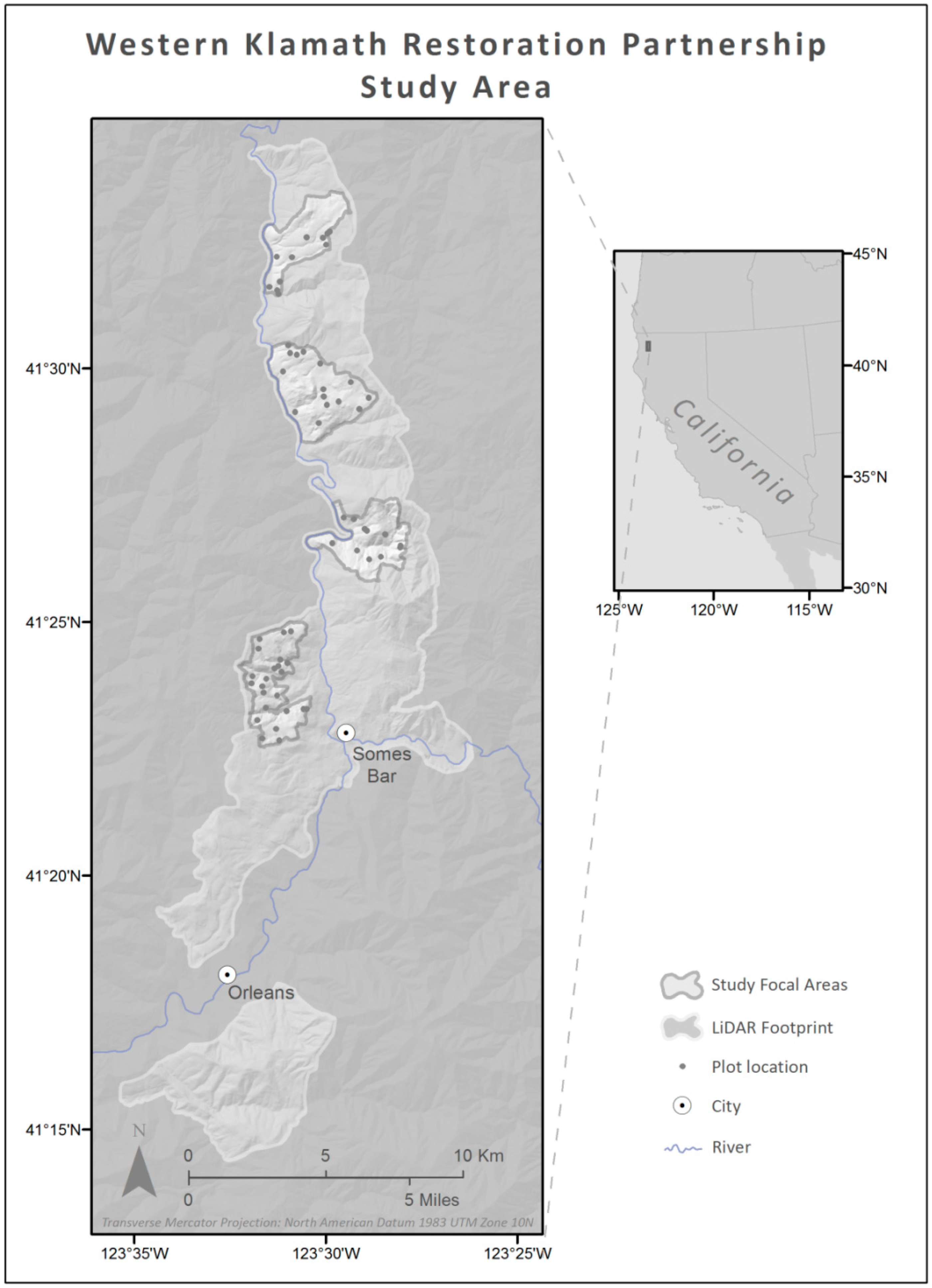
2.1. Study Area
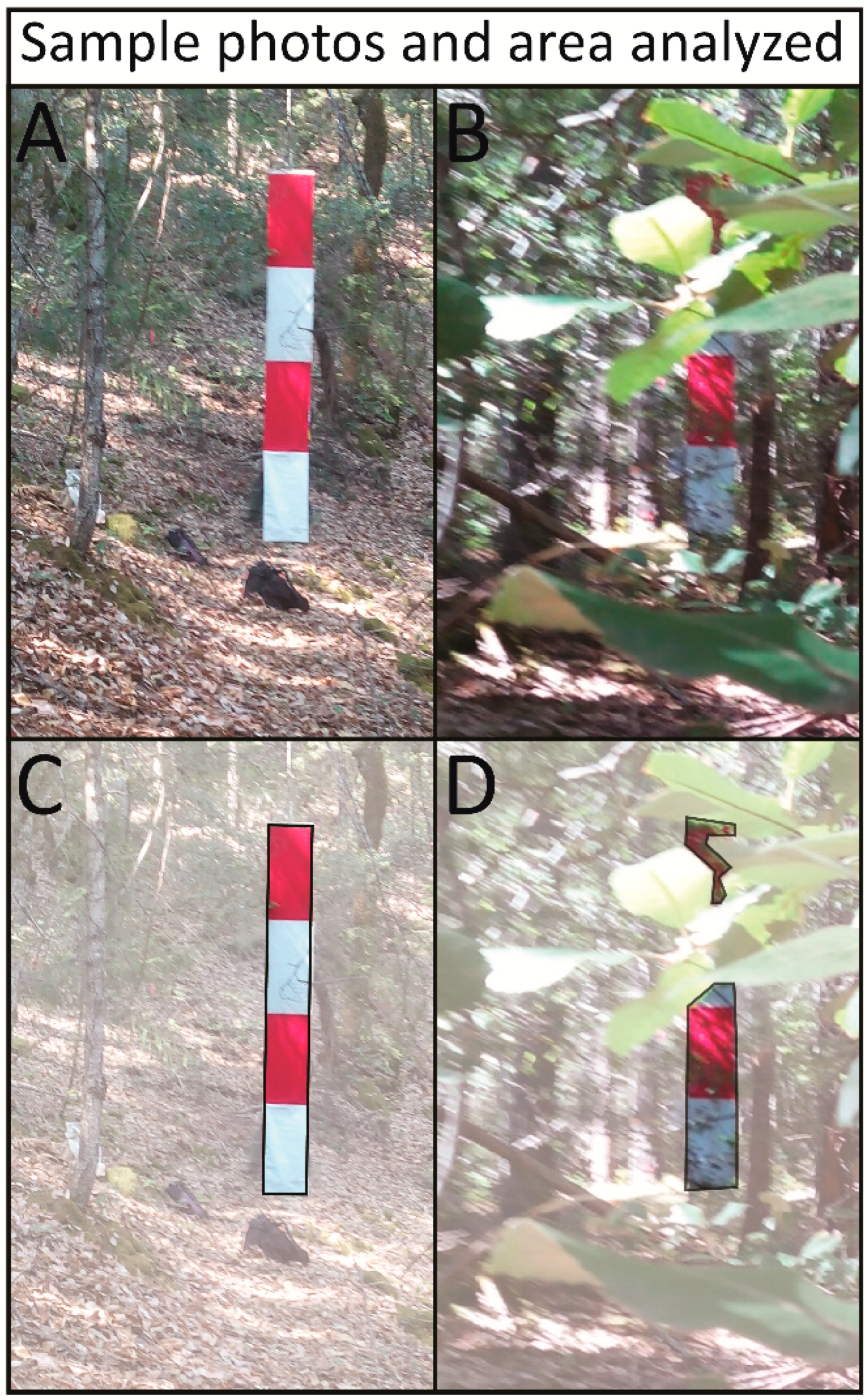
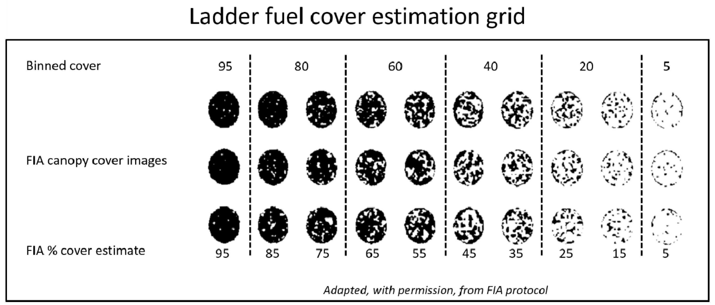
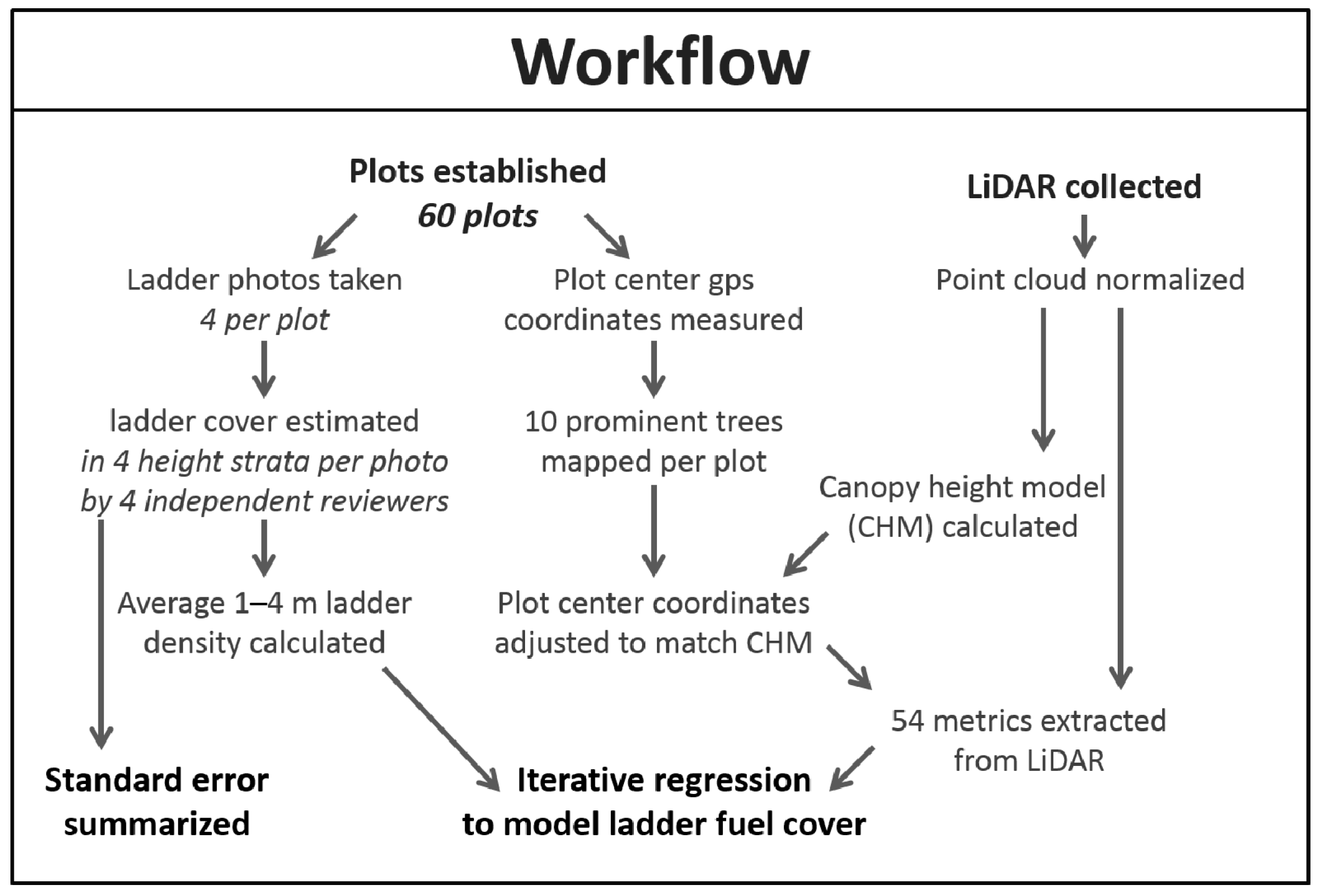
2.2. Field Data
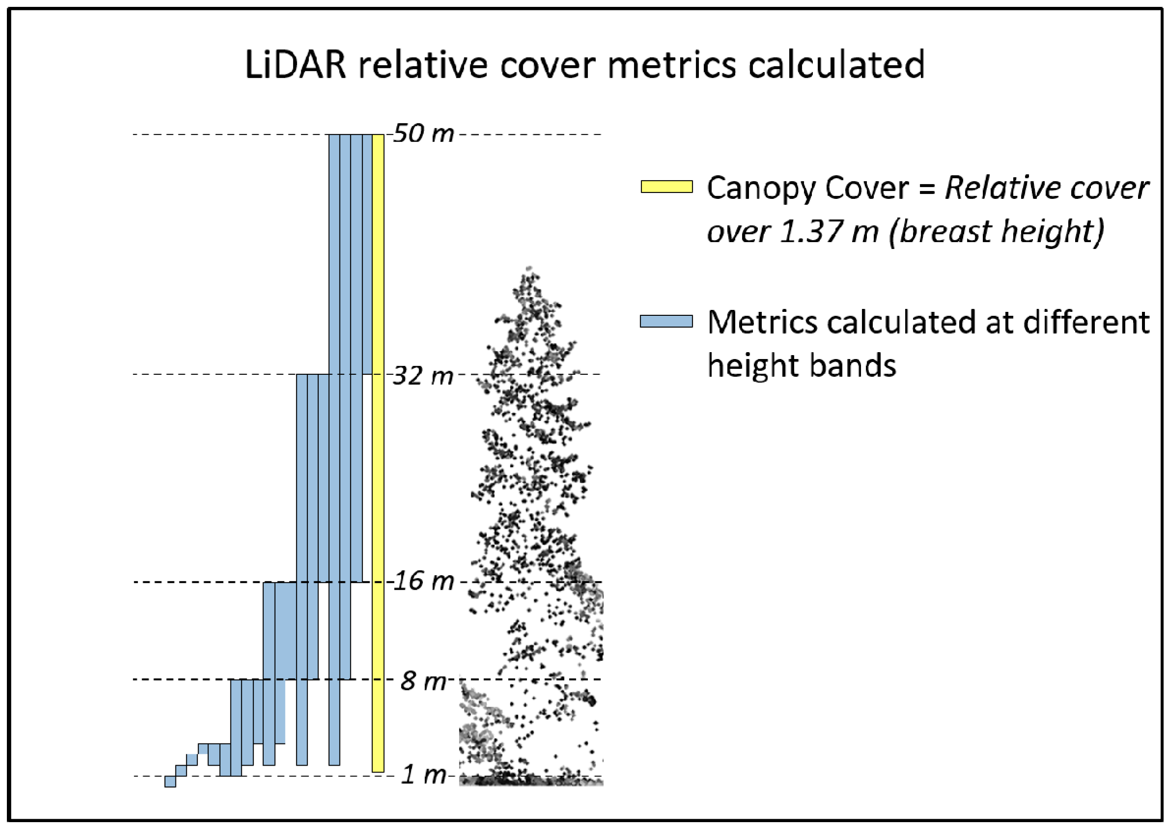
2.3. LiDAR Data and Processing
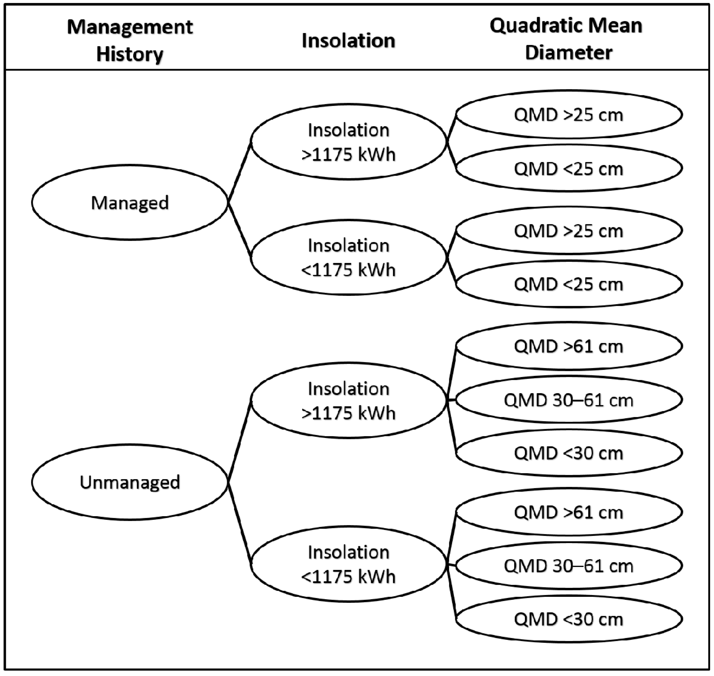
2.4. Statistical Analysis
3. Results
3.1. Assessment of Photo-Banner
3.2. Linking LiDAR to Ground-Based Measures
4. Discussion
4.1. Immediate Implications for Managers
4.2. Study Limitations
4.3. Future Research
5. Conclusions
Acknowledgments
Author Contributions
Conflicts of Interest
Abbreviations
| LiDAR | Light Detection and Ranging |
| CBH | Canopy base height |
| CHM | Canopy height model |
| FIA | Forest Inventory and Analysis |
| RMSE | Root mean squared error |
| COV1_8 | Percentage of all points between 1 and 8 m |
| STD | Standard deviation of point heights above 2 m |
| FCOV8_16 | Percentage of first return points between 8 and 16 m |
| COV1_4 | Percentage of all LiDAR returns between 1 and 4 m |
| COV4_8 | Percentage of all LiDAR returns between 4 and 8 m |
| DBH | Diameter at breast height |
Appendix A

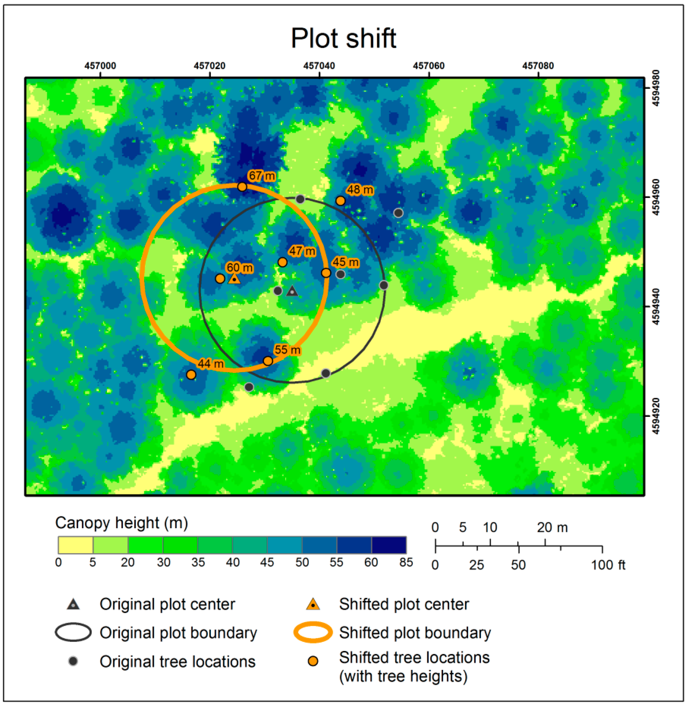
| Plot ID | Horizontal Precision (m) | Distance Shifted (m) |
|---|---|---|
| D001 | 0.7 | 3.2 |
| D104 | 0.2 | 0 |
| D105 | 0.6 | 0.9 |
| D011 | 1.1 | 0 |
| D116 | 0.8 | 1.6 |
| D117 | 0.8 | 2.9 |
| D118 | 0.6 | 0 |
| D124 | 2.2 | 5.1 |
| D126 | 0.8 | 0 |
| D133 | 0.2 | 1.9 |
| D136 | 1.3 | 26.4 |
| D015 | 1 | 3.0 |
| D151 | 1 | 0 |
| D018 | 0.9 | 2.9 |
| D204 | 1 | 0 |
| D234 | 0.8 | 0 |
| D235 | 1.3 | 2.7 |
| D250 | 0.9 | 3.1 |
| D255 | 0.9 | 2.6 |
| D027 | 0.7 | 1.0 |
| D039 | 2.5 | 2.5 |
| D040 | 0.7 | 0.6 |
| D005 | 0.9 | 0 |
| B002 | 1.2 | 10.8 |
| B020 | 1 | 3.3 |
| B021 | 0.3 | 0 |
| B022 | 0.9 | 1.7 |
| B024 | 0.9 | 0 |
| B026 | 0.8 | 0.8 |
| B029 | 0.9 | 2.1 |
| B034 | 1.1 | 3.3 |
| B004 | 0.7 | 1.9 |
| B041 | 0.9 | 1.5 |
| B042 | 0.8 | 1.9 |
| B045 | 0.9 | 3.2 |
| B046 | 0.7 | 6.6 |
| B049 | 0.8 | 0 |
| B050 | 0.9 | 2.8 |
| C033 | 0.8 | 0 |
| C110 | 0.8 | 0 |
| C114 | 0.8 | 2.8 |
| C131 | 0.7 | 3.1 |
| C132 | 1 | 1.3 |
| C139 | 1 | 1.9 |
| C036 | 0.8 | 1.2 |
| C120 | 0.7 | 2.0 |
| C130 | 1 | 1.7 |
| C137 | 0.2 | 2.9 |
| C152 | 0.7 | 1.4 |
| A010 | 0.6 | 0.8 |
| A017 | 0.9 | 4.0 |
| A207 | 0.7 | 2.4 |
| A216 | 0.8 | 3.0 |
| A023 | 0.6 | 5.8 |
| A236 | 0.6 | 1.6 |
| A238 | 1 | 8.2 |
| A043 | 1 | 2.8 |
| A047 | 1.1 | 0 |
| A007 | 0.9 | 2.8 |
| A009 | 0.9 | 0 |
| Variable Group | Individual Variable Description |
|---|---|
| Basic point statistics | Maximum point height |
| Average of point height above 2 m | |
| Quadratic average of point height above 2 m | |
| Skewness of point heights above 2 m | |
| Standard deviation of point heights above 2 m | |
| Kurtosis of point heights above 2 m | |
| Cover by vertical strata calculated for first and all returns = # points in strata _ # points in and below strata | Percentage of points between 1 and 2 m |
| Percentage of points between 2 and 3 m | |
| Percentage of points between 3 and 4 m | |
| Percentage of points between 2 and 4 m | |
| Percentage of points between 1 and 4 m | |
| Percentage of points between 1 and 8 m | |
| Percentage of points between 2 and 8 m | |
| Percentage of points between 4 and 8 m | |
| Percentage of points between 2 and 16 m | |
| Percentage of points between 4 and 16 m | |
| Percentage of points between 8 and 16 m | |
| Percentage of points between 2 and 32 m | |
| Percentage of points between 4 and 32 m | |
| Percentage of points between 8 and 32 m | |
| Percentage of points between 16 and 32 m | |
| Percentage of points over breast height (1.37 m) | |
| Percentage of points over 2 m | |
| Percentage of points over 8 m | |
| Percentage of points over 16 m | |
| Percentage of points over 32 m | |
| Percentile Heights | Height of 5th percentile of points above 2 m |
| Height of 10th percentile of points above 2 m | |
| Height of 25th percentile of points above 2 m | |
| Height of 50th percentile of points above 2 m | |
| Height of 75th percentile of points above 2 m | |
| Height of 90th percentile of points above 2 m | |
| Height of 95th percentile of points above 2 m | |
| Height of 99th percentile of points above 2 m |
References
- Lefsky, M.A.; Cohen, W.B.; Parker, G.G.; Harding, D.J. Lidar remote sensing for ecosystem studies. Bioscience 2002, 52, 19–30. [Google Scholar] [CrossRef]
- Dubayah, R.O.; Drake, J.B. Lidar remote sensing for forestry. J. For. 2000, 98, 44–46. [Google Scholar]
- Arroyo, L.A.; Pascual, C.; Manzanera, J.A. Fire models and methods to map fuel types: The role of remote sensing. For. Ecol. Manag. 2008, 256, 1239–1252. [Google Scholar] [CrossRef] [Green Version]
- Hyyppä, J.; Hyyppä, H.; Inkinen, M.; Engdahl, M.; Linko, S.; Zhu, Y.-H. Accuracy comparison of various remote sensing data sources in the retrieval of forest stand attributes. For. Ecol. Manag. 2000, 128, 109–120. [Google Scholar] [CrossRef]
- Husari, S.; Nichols, T.H.; Sugihara, N.G.; Stephens, S.L. Fire and Fuel Management; University of California Press: Berkeley, CA, USA, 2006; pp. 444–465. [Google Scholar]
- US Forest Service. The Rising Cost of Fire Operations: Effects on the Forest Service’s Non-Fire Work; US Department of Agriculture: Washington, DC, USA, 2015; p. 16.
- Hessburg, P.F.; Agee, J.K.; Franklin, J.F. Dry forests and wildland fires of the inland Northwest USA: Contrasting the landscape ecology of the pre-settlement and modern eras. For. Ecol. Manag. 2005, 211, 117–139. [Google Scholar] [CrossRef]
- Skinner, C.N.; Taylor, A.H.; Agee, J.K. Klamath Mountains Bioregion. In Fire in California Ecosystems; Sugihara, N.S., Van Wagtendonk, J.W., Fites-Kaufman, J., Shaffer, K.E., Thode, A., Eds.; University of California Press: Berkeley, CA, USA, 2006; pp. 170–194. [Google Scholar]
- Miller, J.; Thode, A. Quantifying burn severity in a heterogeneous landscape with a relative version of the delta Normalized Burn Ratio (dNBR). Remote Sens. Environ. 2007, 109, 66–80. [Google Scholar] [CrossRef]
- Miller, J.; Knapp, E.; Key, C.; Skinner, C.; Isbell, C.; Creasy, R.; Sherlock, J. Calibration and validation of the relative differenced Normalized Burn Ratio (RdNBR) to three measures of fire severity in the Sierra Nevada and Klamath Mountains, California, USA. Remote Sens. Environ. 2009, 113, 645–656. [Google Scholar] [CrossRef]
- Miller, J.; Safford, H. Trends in wildfire severity: 1984 to 2010 in the Sierra Nevada, Modoc Plateau, and Southern Cascades, California, USA. Fire Ecol. 2012, 8, 41–57. [Google Scholar] [CrossRef]
- Agee, J.K.; Skinner, C.N. Basic principles of forest fuel reduction treatments. For. Ecol. Manag. 2005, 211, 83–96. [Google Scholar] [CrossRef]
- Menning, K.M.; Stephens, S.L. Fire climbing in the forest: A semiqualitative, semiquantitative approach to assessing ladder fuel hazards. West. J. Appl. For. 2007, 22, 88–93. [Google Scholar]
- Hirsch, K.; Martell, D. A review of initial attack fire crew productivity and effectiveness. Int. J. Wildland Fire 1996, 6, 199–215. [Google Scholar] [CrossRef]
- Norgaard, K.M. The Politics of fire and the social impacts of fire exclusion on the Klamath. Humboldt J. Soc. Relat. 2014, 36, 77–101. [Google Scholar]
- Prichard, S.J.; Sandberg, D.V.; Ottmar, R.D.; Eberhardt, E.; Andreu, A.; Eagle, P.; Swedin, K. Fuel Characteristic Classification System Version 3.0: Technical Documentation. USDA Forest Service; General Technical Report PNW-GTR-887; Pacific Northwest Research Station: Portland, OR, USA, 2013. [Google Scholar]
- Wright, C.S.; Ottmar, R.; Vihnanek, R. Stereo Photo Series for Quantifying Natural Fuels. Volume VIII: Hardwood, Pitch Pine, and Red Spruce/Basam Fire Types in the Northeastern United States; Seventh Symposium on Fire and Forest Meteorology, 2007; US National Wildfire Coordinating Group, National Interagency Fire Center: Boise, ID, USA, 2007; p. 91.
- Scott, J.H.; Reinhardt, E.D. Assessing Crown Fire Potential by Linking Models of Surface and Crown Fire Behavior; Research Paper RMRS-RP-29; USDA Forest Service, Rocky Mountain Research Station: Fort Collins, CO, USA, 2001.
- Reinhardt, E.; Lutes, D.; Scott, J. FuelCalc: A method for estimating fuel characteristics. In Proceedings of the Fuels Management-How to Measure Success: Conference Proceedings, Portland, OR, USA, 28–30 March 2006; USDA Forest Service, Rocky Mountain Research Station: Fort Collins, CO, USA, 2006. [Google Scholar]
- Sando, R.W.; Wick, C.H. A Method of Evaluating Crown Fuels in Forest Stands; RP-NC-84; USDA Forest Service: Ogden, UT, USA, 1972.
- Mitsopoulos, I.D.; Dimitrakopoulos, A.P. Canopy fuel characteristics and potential crown fire behavior in Aleppo pine (Pinus halepensis Mill.) forests. Ann. For. Sci. 2007, 64, 287–299. [Google Scholar] [CrossRef]
- Ottmar, R.D.; Vihnanek, R.E.; Wright, C.S. Stereo Photo Series for Quantifying Natural Fuels, Volume 1: Mixed-Conifer with Mortality, Western Juniper, Sagebrush, and Grassland Types in the Interior Pacific Northwest; US National Wildfire Coordinating Group, National Interagency Fire Center: Boise, ID, USA, 1998; p. 73.
- Fernandes, P.M. Combining forest structure data and fuel modelling to classify fire hazard in Portugal. Ann. For. Sci. 2009, 66, 1–9. [Google Scholar] [CrossRef]
- Erdody, T.L.; Moskal, L.M. Fusion of LiDAR and imagery for estimating forest canopy fuels. Remote Sens. Environ. 2010, 114, 725–737. [Google Scholar] [CrossRef]
- Andersen, H.-E.; McGaughey, R.J.; Reutebuch, S.E. Estimating forest canopy fuel parameters using LIDAR data. Remote Sens. Environ. 2005, 94, 441–449. [Google Scholar] [CrossRef]
- Jakubowski, M.K.; Guo, Q.; Collins, B.; Stephens, S.; Kelly, M. Predicting surface fuel models and fuel metrics using lidar and CIR imagery in a dense, mountainous forest. Photogramm. Eng. Remote Sens. 2013, 79, 37–49. [Google Scholar] [CrossRef]
- Brown, J.K. Weight and Density of Crowns of Rocky Mountain Conifers; Research Paper INT-197; USDA Forest Service, Intermountain Forest and Range Experiment Station: Ogden, UT, USA, 1978.
- Brown, J.K.; Johnston, C.M. Debris Prediction System; Fuel Science RWU 2104; USDA Forest Service, Intermountain Forest and Range Experiment Station: Missoula, MT, USA, 1976.
- Wilson, J.; Baker, P. Mitigating fire risk to late-successional forest reserves on the east slope of the Washington Cascade Range, USA. For. Ecol. Manag. 1998, 110, 59–75. [Google Scholar] [CrossRef]
- Cruz, M.G.; Alexander, M.E.; Wakimoto, R.H. Assessing canopy fuel stratum characteristics in crown fire prone fuel types of western North America. Int. J. Wildland Fire 2003, 12, 39–50. [Google Scholar] [CrossRef]
- McAlpine, R.; Hobbs, M. Predicting the height to live crown base in plantations of four boreal forest species. Int. J. Wildland Fire 1994, 4, 103–106. [Google Scholar] [CrossRef]
- Dean, T.J.; Cao, Q.V.; Roberts, S.D.; Evans, D.L. Measuring heights to crown base and crown median with LiDAR in a mature, even-aged loblolly pine stand. For. Ecol. Manag. 2009, 257, 126–133. [Google Scholar] [CrossRef]
- Hall, S.A.; Burke, I.C.; Box, D.O.; Kaufmann, M.R.; Stoker, J.M. Estimating stand structure using discrete-return lidar: An example from low density, fire prone ponderosa pine forests. For. Ecol. Manag. 2005, 208, 189–209. [Google Scholar] [CrossRef]
- Rebain, S.A. The Fire and Fuels Extension to the Forest Vegetation Simulator: Updated Model. Documentation; USDA Forest Service Internal Report; Forest Management Service Center: Fort Collins, CO, USA, 2010.
- Mitsopoulos, I.; Dimitrakopoulos, A. Estimation of canopy fuel characteristics of Aleppo pine (Pinus halepensis Mill.) forests in Greece based on common stand parameters. Eur. J. For. Res. 2014, 133, 73–79. [Google Scholar] [CrossRef]
- Cruz, M.G.; Alexander, M.E.; Wakimoto, R.H. Modeling the likelihood of crown fire occurrence in conifer forest stands. For. Sci. 2004, 50, 640–658. [Google Scholar]
- Hall, S.A.; Burke, I.C. Considerations for characterizing fuels as inputs for fire behavior models. For. Ecol. Manag. 2006, 227, 102–114. [Google Scholar] [CrossRef]
- Kramer, H.A.; Collins, B.M.; Kelly, M.; Stephens, S.L. Quantifying ladder fuels: A new approach using LiDAR. Forests 2014, 5, 1432–1453. [Google Scholar] [CrossRef]
- Nudds, T.D. Quantifying the vegetative structure of wildlife cover. Wildl. Soc. Bull. 1977, 5, 113–117. [Google Scholar]
- Jones, R.E. A board to measure cover used by prairie grouse. J. Wildl. Manag. 1968, 32, 28–31. [Google Scholar] [CrossRef]
- Griffith, B.; Youtie, B.A. Two devices for estimating foliage density and deer hiding cover. Wildl. Soc. Bull. 1988, 16, 206–210. [Google Scholar]
- Brown, J.D.; Benson, T.J.; Bednarz, J.C. Vegetation characteristics of Swainson’s warbler habitat at the white river national wildlife refuge, Arkansas. Wetlands 2009, 29, 586–597. [Google Scholar] [CrossRef]
- Duebbert, H.F.; Lokemoen, J.T. Duck nesting in fields of undisturbed grass-legume cover. J. Wildl. Manag. 1976, 40, 39–49. [Google Scholar] [CrossRef]
- Huegel, C.N.; Dahlgren, R.B.; Gladfelter, H.L. Bedsite selection by white-tailed deer fawns in Iowa. J. Wildl. Manag. 1986, 50, 474–480. [Google Scholar] [CrossRef]
- Hyde, E.J.; Simons, T.R. Sampling plethodontid salamanders: Sources of variability. J. Wildl. Manag. 2001, 65, 624–632. [Google Scholar] [CrossRef]
- Lefsky, M.A.; Cohen, W.B.; Acker, S.A.; Parker, G.G.; Spies, T.A.; Harding, D. Lidar remote sensing of the canopy structure and biophysical properties of Douglas-fir Western Hemlock Forests. Remote Sens. Environ. 1999, 70, 339–361. [Google Scholar] [CrossRef]
- Kelly, M.; Di Tommaso, S. Mapping forests with Lidar provides flexible, accurate data with many uses. Calif. Agric. 2015, 69, 14–20. [Google Scholar] [CrossRef]
- Coops, N.C.; Hilker, T.; Wulder, M.A.; St-Onge, B.; Newnham, G.; Siggins, A.; Trofymow, J.A. Estimating canopy structure of Douglas-fir forest stands from discrete-return LiDAR. Trees 2007, 21, 295–310. [Google Scholar] [CrossRef]
- Kane, V.R.; Bakker, J.D.; McGaughey, R.J.; Lutz, J.A.; Gersonde, R.F.; Franklin, J.F. Examining conifer canopy structural complexity across forest ages and elevations with LiDAR data. Can. J. For. Res. 2010, 40, 774–787. [Google Scholar] [CrossRef]
- Riaño, D.; Chuvieco, E.; Condés, S.; González-Matesanz, J.; Ustin, S.L. Generation of crown bulk density for Pinus sylvestris L. from lidar. Remote Sens.Environ. 2004, 92, 345–352. [Google Scholar] [CrossRef]
- Richardson, J.J. Estimating leaf area index from multiple return, small-footprint aerial lidar at the Washington Park Arboretum. Agric. For. Meteorol. 2008, 149, 1152–1160. [Google Scholar] [CrossRef]
- Jensen, J.; Humes, K.; Vierling, L.; Hudak, A. Discrete return lidar-based prediction of leaf area index in two conifer forests. Remote Sens. Environ. 2008, 112, 3947–3957. [Google Scholar] [CrossRef]
- Kane, V.R.; North, M.P.; Lutz, J.A.; Churchill, D.J.; Roberts, S.L.; Smith, D.F.; McGaughey, R.J.; Kane, J.T.; Brooks, M.L. Assessing fire effects on forest spatial structure using a fusion of Landsat and airborne LiDAR data in Yosemite National Park. Remote Sens. Environ. 2014, 151, 89–101. [Google Scholar] [CrossRef]
- Zhao, F.; Sweitzer, R.A.; Guo, Q.; Kelly, M. Characterizing habitats associated with fisher den structures in the Southern Sierra Nevada, California using discrete return lidar. For. Ecol. Manag. 2012, 280, 112–119. [Google Scholar] [CrossRef]
- Garcı, C.; Tempel, D.J.; Kelly, M. LiDAR as a tool to characterize wildlife habitat: California spotted Owl nesting habitat as an example. J. For. 2011, 109, 436–443. [Google Scholar]
- Mutlu, M.; Popescu, S.C.; Zhao, K. Sensitivity analysis of fire behavior modeling with LIDAR-derived surface fuel maps. For. Ecol. Manag. 2008, 256, 289–294. [Google Scholar] [CrossRef]
- Mutlu, M.; Popescu, S.; Stripling, C.; Spencer, T. Mapping surface fuel models using lidar and multispectral data fusion for fire behavior. Remote Sens. Environ. 2008, 112, 274–285. [Google Scholar] [CrossRef]
- Riano, D.; Meier, E.; Allgöwer, B.; Chuvieco, E.; Ustin, S.L. Modeling airborne laser scanning data for the spatial generation of critical forest parameters in fire behavior modeling. Remote Sens. Environ. 2003, 86, 177–186. [Google Scholar] [CrossRef]
- Wing, B.M.; Ritchie, M.W.; Boston, K.; Cohen, W.B.; Gitelman, A.; Olsen, M.J. Prediction of understory vegetation cover with airborne lidar in an interior ponderosa pine forest. Remote Sens. Environ. 2012, 124, 730–741. [Google Scholar] [CrossRef]
- Skowronski, N.; Clark, K.; Nelson, R.; Hom, J.; Patterson, M. Remotely sensed measurements of forest structure and fuel loads in the Pinelands of New Jersey. Remote Sens. Environ. 2007, 108, 123–129. [Google Scholar] [CrossRef]
- Taylor, A.H.; Skinner, C.N. Fire history and landscape dynamics in a late-successional reserve, Klamath Mountains, California, USA. For. Ecol. Manag. 1998, 111, 285–301. [Google Scholar] [CrossRef]
- Cheng, S. Forest Service Research Natural Areas in California; General Technical Report PSW-GTR-188; Pacific Southwest Research Station, Forest Service, U.S. Department of Agriculture: Albany, CA, USA, 2004.
- Davis, B.; Hendryx, M. Plants and the People: The Ethnobotany of the Karuk Tribe; Siskiyou County Museum: Yreka, CA, USA, 2004; p. 166. [Google Scholar]
- Lake, F.K. Historical and cultural fires, tribal management and research issue in Northern California: Trails, fires and tribulations. Interdiscip. Stud. Humanit. 2013, 5, 22. [Google Scholar]
- Whittaker, R.H. Vegetation of the Siskiyou mountains, Oregon and California. Ecol. Monogr. 1960, 30, 279–338. [Google Scholar] [CrossRef]
- Miller, J.; Skinner, C.; Safford, H.; Knapp, E.E.; Ramirez, C. Trends and causes of severity, size, and number of fires in northwestern California, USA. Ecol. Appl. 2012, 22, 184–203. [Google Scholar] [CrossRef] [PubMed]
- Skinner, C.N. Change in spatial characteristics of forest openings in the Klamath Mountains of northwestern California, USA. Landsc. Ecol. 1995, 10, 219–228. [Google Scholar] [CrossRef]
- USDA Forest Service—Pacific Southwest Region—Remote Sensing Lab. CalvegTiles_Ecoregions07_4. 2010. Available online: http://www.fs.fed.us/r5/rsl/clearinghouse/gis-download.shtml (accessed on 18 May 2015).
- Bennett, L.T.; Judd, T.S.; Adams, M.A. Close-range vertical photography for measuring cover changes in perennial grasslands. J. Range Manag. 2000, 53, 634–641. [Google Scholar] [CrossRef]
- Schomaker, M.E.; Zarnoch, S.J.; Bechtold, W.A.; Latelle, D.J.; Burkman, W.G.; Cox, S.M. Crown-Condition Classification: A Guide to Data Collection and Analysis; Department of Agriculture, Forest Service, Southern Research Station: Asheville, NC, USA, 2007; p. 78.
- Quantum Spatial. Lower Klamath Watersheds LiDAR & Digital Imagery: Technical Data Report Summary; QSI Environmental: Corvallis, OR, USA, 2015; p. 42. [Google Scholar]
- Isenburg, M. LAStools—Efficient Tools for LiDAR Processing. 2011. Available online: http://lastools.org (accessed on 16 October 2015).
- R Development Core Team. R: A Language and Environment for Statistical Computing; R Foundation for Statistical Computing: Vienna, Austria, 2008. [Google Scholar]
- Keane, R.E.; Gray, K.; Bacciu, V.; Leirfallom, S. Spatial scaling of wildland fuels for six forest and rangeland ecosystems of the northern Rocky Mountains, USA. Landsc. Ecol. 2012, 27, 1213–1234. [Google Scholar] [CrossRef]
- Kane, V.R.; Lutz, J.A.; Roberts, S.L.; Smith, D.F.; McGaughey, R.J.; Povak, N.A.; Brooks, M.L. Landscape-scale effects of fire severity on mixed-conifer and red fir forest structure in Yosemite National Park. For. Ecol. Manag. 2013, 287, 17–31. [Google Scholar] [CrossRef]
- McGaughey, R. FUSION/LDV: Software for LIDAR Data Analysis and Visualization, Version 3.01; USDA Forest Service, Pacific Northwest Research Station, University of Washington: Seattle, WA, USA, 2012.
- Hudak, A.T.; Crookston, N.L.; Evans, J.S.; Falkowski, M.J.; Smith, A.M.S.; Gessler, P. Regression modeling and mapping of coniferous forest basal area and tree density from discrete-return LiDAR and multispectral satellite data. Can. J. Remote Sens. 2006, 32, 126–138. [Google Scholar] [CrossRef]
- Hudak, A.T.; Strand, E.K.; Vierling, L.A.; Byrne, J.C.; Eitel, J.U.; Martinuzzi, S.; Falkowski, M.J. Quantifying aboveground forest carbon pools and fluxes from repeat LiDAR surveys. Remote Sens. Environ. 2012, 123, 25–40. [Google Scholar] [CrossRef]
- Lumley, T.; Miller, A. Leaps: Regression Subset Selection. R package version 2.9. 2009. Available online: http://CRAN.R-project.org/package=leaps (accessed on 12 November 2014).
- Breusch, T.S.; Pagan, A.R. A simple test for heteroscedasticity and random coefficient variation. Econom. J. Econom. Soc. 1979, 47, 1287–1294. [Google Scholar] [CrossRef]
- Alfons, A. cvTools: Cross-Validation Tools for Regression Models. R Package Version 0.3.2. 2012. Available online: https://cran.r-project.org/web/packages/cvTools/index.html (accessed on 12 November 2014).
- Zimble, D.A.; Evans, D.L.; Carlson, G.C.; Parker, R.C.; Grado, S.C.; Gerard, P.D. Characterizing vertical forest structure using small-footprint airborne LiDAR. Remote Sens. Environ. 2003, 87, 171–182. [Google Scholar] [CrossRef]
- Vaillant, N.M.; Noonan-Wright, E.; Dailey, S.; Ewell, C.; Reiner, A. Effectiveness and longevity of fuel treatments in coniferous forests across California. JFSP Res. Proj. Rep. 2013, 57, 29. [Google Scholar]
- Harling, W.; Tripp, B. Western Klamath Restoration Partnership: A Plan for Restoring Fire Adapted Landscapes; Western Klamath Restoration Partnership; MKWC: Orleans, CA, USA, 2014; p. 57. [Google Scholar]
- Skowronski, N.S.; Clark, K.L.; Duveneck, M.; Hom, J. Three-dimensional canopy fuel loading predicted using upward and downward sensing LiDAR systems. Remote Sens. Environ. 2011, 115, 703–714. [Google Scholar] [CrossRef]
- Seielstad, C.A.; Queen, L.P. Using airborne laser altimetry to determine fuel models for estimating fire behavior. J. For. 2003, 101, 10–15. [Google Scholar]
- Popescu, S.C.; Zhao, K. A voxel-based lidar method for estimating crown base height for deciduous and pine trees. Remote Sens. Environ. 2008, 112, 767–781. [Google Scholar] [CrossRef]
- Zielinski, W.J.; Dunk, J.R.; Yaeger, J.S.; LaPlante, D.W. Developing and testing a landscape-scale habitat suitability model for fisher (Martes pennanti) in forests of interior northern California. For. Ecol. Manag. 2010, 260, 1579–1591. [Google Scholar] [CrossRef]
- Hummel, S.; Lake, F. Forest site classification for cultural plant harvest by tribal weavers can inform management. J. For. 2015, 113, 30–39. [Google Scholar] [CrossRef]
- Anderson, K. Tending the Wild: Native American Knowledge and the Management of California's Natural Resources; University of California Press: Oakland, CA, USA, 2005. [Google Scholar]
- Long, J.W.; Quinn-Davidson, L.; Goode, R.W.; Lake, F.K.; Skinner, C.N. Restoring California Black Oak to Support Tribal Values and Wildlife. In Proceedings of the 7th California Oak Symposium: Managing Oak Woodlands in a Dynamic World; Department of Agriculture, Forest Service, Pacific Southwest Research Station: Albany, CA, USA, 2015; pp. 113–122. [Google Scholar]
- Lake, F.K.; Long, J.W. Fire and Tribal Cultural Resources; Department of Agriculture, Forest Service, Pacific Southwest Research Station: Albany, CA, USA, 2014; pp. 173–186.
- Burger, J.; Gochfeld, M.; Pletnikoff, K.; Snigaroff, R.; Snigaroff, D.; Stamm, T. Ecocultural attributes: Evaluating ecological degradation in terms of ecological goods and services versus subsistence and tribal values. Risk Anal. 2008, 28, 1261–1272. [Google Scholar] [CrossRef] [PubMed]
- Barbour, R.J.; Singleton, R.; Maguire, D.A. Evaluating forest product potential as part of planning ecological restoration treatments on forested landscapes. Landsc. Urban Plan. 2007, 80, 237–248. [Google Scholar] [CrossRef]
- Kane, V.R.; Cansler, C.A.; Povak, N.A.; Kane, J.T.; McGaughey, R.J.; Lutz, J.A.; Churchill, D.J.; North, M.P. Mixed severity fire effects within the Rim fire: Relative importance of local climate, fire weather, topography, and forest structure. For. Ecol. Manag. 2015, 358, 62–79. [Google Scholar] [CrossRef]
- Hoiem, D.; Efros, A.A.; Hebert, M. Putting objects in perspective. Int. J. Comput. Vis. 2008, 80, 3–15. [Google Scholar] [CrossRef]
- Kramer, H.A.; Collins, B.M.; Gallagher, C.V.; Keane, J.; Kelly, M.; Stephens, S.L. Accessible LiDAR: Estimating large tree density for habitat identification. 2016; under review. [Google Scholar]


| 2 Photos | 3 Photos | 4 Photos | ||||
|---|---|---|---|---|---|---|
| Height bin | Average | Maximum | Average | Maximum | Average | Maximum |
| 0–1 m | 8.24 | 30.00 | 9.09 | 24.73 | 8.10 | 19.51 |
| 1–2 m | 8.84 | 41.25 | 7.95 | 23.75 | 7.72 | 19.46 |
| 2–3 m | 9.34 | 32.50 | 7.54 | 21.79 | 6.44 | 15.72 |
| 3–4 m | 9.94 | 37.50 | 7.67 | 22.42 | 6.79 | 15.54 |
| Ladder Fuel Cover | FCOV8_16 | COV1_4 | COV1_8 | COV4_8 | STD | |
|---|---|---|---|---|---|---|
| Ladder fuel cover | 1 | - | - | - | - | - |
| FCOV8_16 | 0.36 | 1 | - | - | - | - |
| COV1_4 | 0.69 | 0.59 | 1 | - | - | - |
| COV1_8 | 0.79 | 0.37 | 0.88 | 1 | - | - |
| COV4_8 | 0.74 | 0.05 | 0.54 | 0.86 | 1 | - |
| STD | 0.22 | 0.34 | 0.25 | 0.05 | 0.25 | 1 |
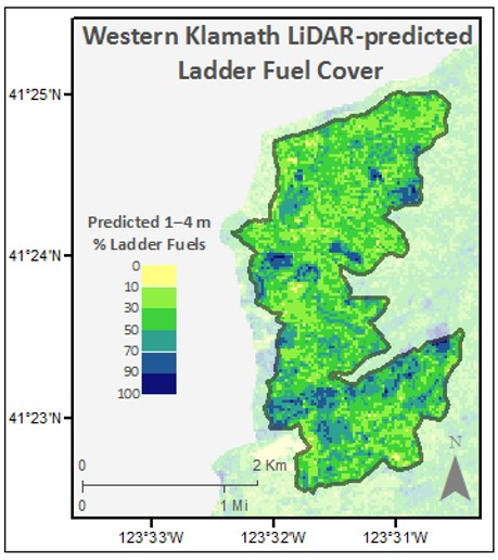
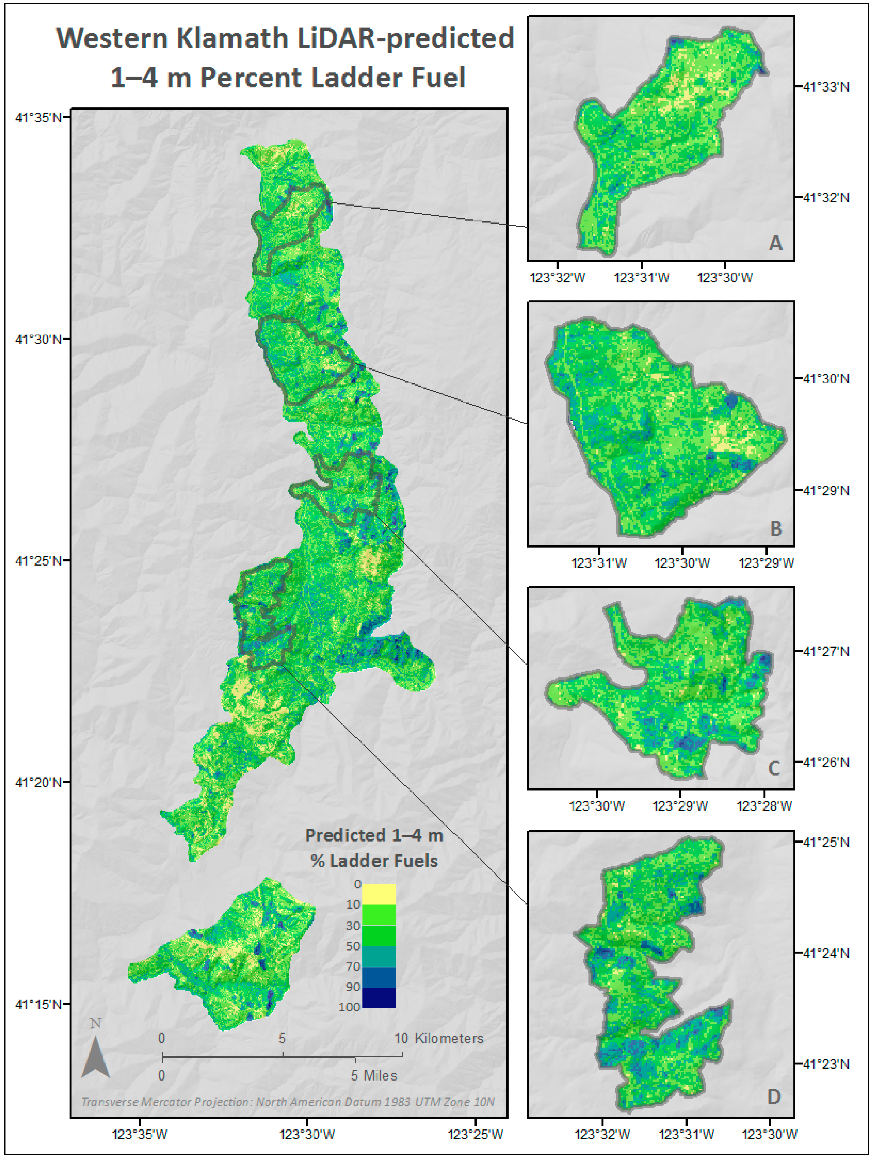
| Focal Area | Average Ladder Fuel Cover (%) | % Area Above 90th Percentile Ladder Fuel Cover |
|---|---|---|
| A | 31.53 | 3.89 |
| B | 36.27 | 6.59 |
| C | 36.61 | 10.23 |
| D | 40.99 | 16.02 |
© 2016 by the authors; licensee MDPI, Basel, Switzerland. This article is an open access article distributed under the terms and conditions of the Creative Commons Attribution (CC-BY) license (http://creativecommons.org/licenses/by/4.0/).
Share and Cite
Kramer, H.A.; Collins, B.M.; Lake, F.K.; Jakubowski, M.K.; Stephens, S.L.; Kelly, M. Estimating Ladder Fuels: A New Approach Combining Field Photography with LiDAR. Remote Sens. 2016, 8, 766. https://0-doi-org.brum.beds.ac.uk/10.3390/rs8090766
Kramer HA, Collins BM, Lake FK, Jakubowski MK, Stephens SL, Kelly M. Estimating Ladder Fuels: A New Approach Combining Field Photography with LiDAR. Remote Sensing. 2016; 8(9):766. https://0-doi-org.brum.beds.ac.uk/10.3390/rs8090766
Chicago/Turabian StyleKramer, Heather A., Brandon M. Collins, Frank K. Lake, Marek K. Jakubowski, Scott L. Stephens, and Maggi Kelly. 2016. "Estimating Ladder Fuels: A New Approach Combining Field Photography with LiDAR" Remote Sensing 8, no. 9: 766. https://0-doi-org.brum.beds.ac.uk/10.3390/rs8090766