Catenary System Detection, Localization and Classification Using Mobile Scanning Data

Abstract

This paper presents a new method for detecting, locating and classifying overhead contact systems (catenary systems) in point clouds collected by mobile mapping systems (MMS) on rail roads. Contrary to many other application types, railway embankments are highly regulated and standardized. Railway infrastructure geometric relations remain roughly unchanged within established regions and have similarities between them. The newly-developed method exploits both these characteristics, as well as the survey process. There are several steps in this approach. Firstly, it restricts the search for catenaries relative to the distance to registered MMS trajectory, then finds possible support structures according to the density of points above the track. Subsequently, the method verifies the structures’ presence and classifies the points with the use of the RANSAC algorithm. It establishes the presence of cantilevers, as well as poles or structural beams, depending on the type of detected support structure. The method also determines the coordinates of the identified object on the ground. Finally, a classification is clarified with the use of a modified DBSCAN algorithm. The design method has been verified with data collected in four surveys where the cumulative length of the route was almost 90 km. Over 97% of support structures were correctly detected, and out of these, over 95% were completely classified.

1. Introduction

Mobile laser scanning (MLS) has become quite popular in recent years and has numerous applications. Technology is advancing, and current mobile mapping system (MMS) accuracies allow them to be used in almost any survey mission.

Although there are a wide range of MMS systems providing large amounts of data (Figure 1), there are far fewer algorithms and methods able to automatically process the data. Various research has been done on the automatic processing of point clouds collected by airborne scanners [1,2]. There are also many scientific studies on the detection of primitives or specifically-shaped objects in point clouds [3,4]. Some of them can be implemented in processing MLS point clouds. However, as these data are different due to the specific collection process, view perspective and density variation [5,6], further research into the subject is needed.

There are various types of works that can be conducted using MLS. The first MMS were stabilized on cars [7] and subsequently have had numerous applications already implemented in road maintenance. MLS can be used to take stock and measure the position of road infrastructure elements [8,9,10]. Data obtained by terrestrial MMS can also be used to create a spatial database [11], to carry out road safety inspections [12,13], to model the road area [14], to detect voids and cracks in the pavement [8] and to detect road signs [15,16]. LiDAR technology is also used in the evaluation of road infrastructure, such as tunnels, bridges or retaining walls [17,18,19]. MMS were later adapted to rail cars.

There are 1,021,457 km of railway lines world-wide [20]. In Europe, where rail routes first emerged, there are 349,365 km of tracks [20], of which 19,617 km are in Poland [21]. Rail transport remains one of the most cost-effective and most ecological type of transportation compared to other types. The existence and also the competitiveness of railways in relation to other modes of transport requires constant monitoring. There are several types of surveys that have to be carried out regularly. Surveys include assessing track parameters, such as chainage, cant, twist, gradients, gauge and also clearance gauge monitoring [22]. Current accuracies of point clouds collected by MMS on rails make it possible to use it in clearance gauge monitoring [23] or for the purpose of 3D railroad corridor creation [6]. Traditionally, this type of work was done using a trolley operated by an operator walking on foot [22,24,25,26]. MLS provides data far faster, but while the trolley operator decides what is important to measure, point clouds include multiple measurements to single objects, both those of the utmost importance and those that are redundant. With the existing technology, massive amounts of data are obtained after each survey mission, the processing of which still requires a lot of manual, tedious work. Therefore, the next step in the development of MMS for railways is to automate the data processing.

Railway infrastructure monitoring requires methods that are efficient both at the stage of data collection, as well as at the stage of data processing. Therefore, the data processing algorithm must be, in addition to reliable, highly efficient computationally. The amount of data necessitated the development of an algorithm that is both simple and effective. It is true that the processing of large datasets can be accelerated by the use of high-performance computing farms, but simplicity is always an advantage. The demand for efficient monitoring of railway infrastructures will grow, as will the requirement for MLS. The amount of MLS data is growing and will always be an obstacle on the road to high performance. Simplicity and efficiency were very important criteria in the development of the algorithm.

This work’s goal is to automate the detection of the most common objects within the rail bed, the catenary system. This includes extracting a class of points collected on objects belonging to the catenary, contact cables, catenary wires and support structures and also determining the position of the detected support structures on the ground. For the method to be useful to railway operators, it has to be able to process data collected in various environments and from various MMS on the rail. It has to be efficient, precise and easily tuned to certain object properties. Algorithms with all of these features could have many applications. It could help determine if the catenary does not jeopardize railway safety, help with creating inventories, narrow down the data for processing during safety inspections and also prepare data for automatic railway corridor modelling. To achieve all of these objectives, a prototype method was created that uses simple calculations and relies only on the geometrical parameters of the sought after objects. The method is a sequential filtration process that is heuristic in its core. All parameters and thresholds in the algorithm can be easily tuned to specific data by the end user.

The structure of the paper is as follows. Firstly, there is a brief summary of existing methods (Section 2). Secondly, the basic characteristics and properties of a catenary system are presented (Section 3.1). Section 3.2 contains the algorithm structure description in detail, data preparation (Section 3.2.1), density analysis (Section 3.2.2.), verification of the detected support structures and their location (Section 3.2.3) and classification clarification (Section 3.2.4). The algorithm test data are described in Section 4. Lastly, the results of experimental tests and a discussion are presented (Section 5). Conclusions are made in Section 6.

2. Related Work

The ideas of how to automatically process MMS point clouds collected for road and railroad are quite similar; therefore, algorithms created for both environments have been included in this section.

Most algorithms, created to help automate the processing of point clouds acquired by MSL, relate to the detection of road pavements and road curbs. These algorithms usually utilize characteristics both of the measuring sensors and the object of evaluation. Basic assumptions for most methods are: the road must be an almost flat surface with a locally small slope; curbs must be in its immediate vicinity and have a predetermined height difference [8,9]. Described methods usually fall into one of two groups, firstly, a local analysis approach and, secondly, a global approach. The first group includes all detection algorithms whose base concept is analysis in small point cloud subsets, sections perpendicular to the trajectory or subsequent profiles recorded by the scanner [11,12,27,28]. Then, the algorithms detect the road pavements and curbs using the sliding window method [27] or their position directly under the trajectory and slight changes in altitude or fitting a line [9,11,12,28]. Global approaches are a bit more diverse. Some use road geometry and position, flat and below the trajectory [13]; others use a depth image to filter out points with significant elevation change in the near vicinity [14]. In other research, the surface is found by using morphological operations (erosion) [29]. A very interesting approach was presented in [5], where the authors search for road pavements and facades using the geometric index calculated using the roughness value.

The detection of slender vertical objects may include: power poles, lanterns, sign posts and trees. The determination of the position of these objects is used in the inventory of roads [8], surveying [13], as well as to improve the accuracy of automatic navigating vehicles [30]. Depending on the application and its data, algorithms are structured differently. There are more general methods, designed to detect all pole-shaped objects near to roads [5,30,31], or more specialized, for traction poles only [32]. Methods for detecting pole-like objects in point clouds differ vastly, though most use at least two-step procedures, where the first step consists of some type of segmentation or restriction of the search area. A couple of algorithms propose two-step procedures with segmentation in voxels first and then the actual search for pole-like objects [5,30]. Another method was proposed in [31], where point clouds are analyzed in single scanner profiles. Short circular sweeps that are removed from the rest of the data and presented directly above each other in subsequent profiles are classified as poles. An algorithm with a slightly wider application presented in [33] detects poles and other objects near roads using derived object features, both shape and context.

Processing of point clouds collected for railroads include mostly rail detection [34,35,36,37,38,39], sometimes catenary wires [34,36,39] and catenary support structures [6,32,36,39]. Similar to methods described earlier, most algorithms limit the search area in point clouds, by segmentation, buffering or a basic classification process. For this purpose, some algorithms use the approximated position derived from orthophotomaps [35], embankments detected by moving window operators [38] or the trajectory of the MLS [32,36]. Actual rail detection is usually performed by the local analysis of elevation differences [5,34,35,37,38,39], but there are also methods that involve using the fitting of the rail model into the data [36] or search by the continuity and parallel position properties of rails [38]. Methods using the analysis of local height jumps have their drawbacks: they often incorrectly classify points belonging to the railway sleepers or various railway line control devices [37]. For this reason, some methods include an additional verification step.

Catenary detection and classification are done usually by limiting the distance vertically and horizontally from the previously-detected rails or system trajectory [32,34,36]. Verification of detected overhead wires is performed using a simplified model to fit into detected rails and catenary in the planar horizontal view [34] or by usage of the RANSAC algorithm combined with intensity values [36]. Catenary cables are also detected by a point neighborhood check together with other derived geometric features [39]. Other methods used to find objects similar to catenary wires include powerline searches. In [40,41], powerlines, typical properties, neighborhood, continuity and detachment are used to locate them. To verify found objects, polynomial functions are used to fit the model.

Support structures are detected by several algorithms [6,32,39]. Each method approaches the problem differently. Pastucha [32] localize support structures along the corridor with a density check over the rail track, but do not perform classification. Arastounia [39] calculates points neighborhoods and recognizes objects by their geometrical properties and topological relationships. Zhu [6] implement rasterization of point clouds into a digital image, and then use digital image processing.

3. Methodology

3.1. Geometrical Properties and Spatial Relations

The objective of this work is to automatically detect and classify points belonging to the catenary system within the registered track. This includes classifying the points registered on any object belonging to the rail catenary system and locating its support structure. The overhead contact system provides the railway cars with the necessary electric power. The whole system consists of a series of objects. Those taken into consideration in railway gauge clearance monitoring can be divided into two basic groups, cables and support structures. The cables include catenary wires, contact wires and return wires (Figure 2).

There are many different types of support structures, with various construction, material and technical solutions. Due to the number of tracks connected to said structure, they can be divided into two categories, the single solution and the multi-track solution (Figure 3).

Analysis of the rail catenary system provides several clear geometrical observations.

• The relative position of the catenary wires and the rails remains roughly the same throughout the whole route.
• Traction masts or portal structures are placed in fairly regular intervals.
• The connections between the catenary wires and the support system are achieved by cantilevers, which protrude over the rail track. The main axis of each cantilever is roughly perpendicular to the track direction.
• The support structures, both single mast and portal structures, are constructed from beam-like elements, which are either vertical or horizontal.

The designed method tries to incorporate these geometric characteristics into the process in order to make it quicker and more efficient. As the relative position of the catenary wires and the system trajectory remains roughly the same throughout the whole route, the search for overhead cables can be limited to a narrow corridor of data (Figure 4). Additionally, as the cantilevers intrude into this spatial range, they cause a local increase of point density. In this way, a set of possible support structures can be detected. Then, to verify detection, several criteria can be established, based on the support structure characteristics.

3.2. Algorithm Structure

The whole algorithm has been divided into four consecutive steps. The first two steps are relatively easy and rely solely on the typical properties of the railway environment. The first sets up parameters and organizes the data in order to simplify and order the calculations. The second step conducts the calculations to extract the possible support structures from the whole point cloud. The last two steps conduct the calculations locally in order to verify the objects detected, classify the points and clarify their classification. The simplified algorithm structure is shown in Figure 5.

3.2.1. Data Preparation

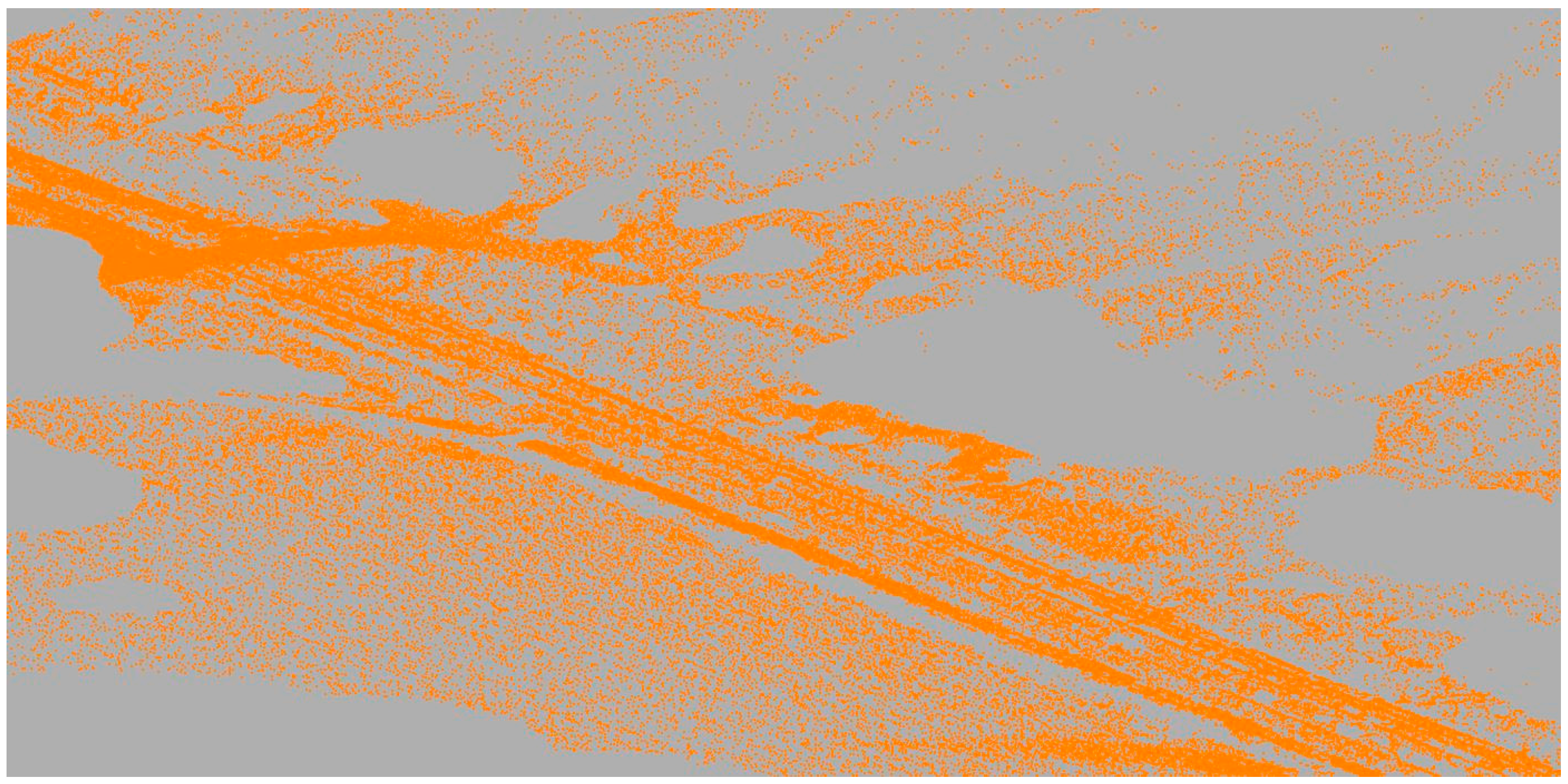
Data preparation consists of the following three procedures, ground filtering, reducing point cloud size and setting the calculation order. Firstly, ground filtering has to be performed. This procedure is necessary for calculating the coordinates of the detected support structure on the ground. The classification might be executed by a number of algorithms, but as it was not the main goal of this work, it was decided to use ground classification algorithms found in the TerraScan software (version 016.003). The results show typical holes in the terrain that arise due to the occlusions (Figure 6). As the classification objective is to provide the elevation coordinates for the positions of the support structures situated directly next to the rail track, the results are sufficient.

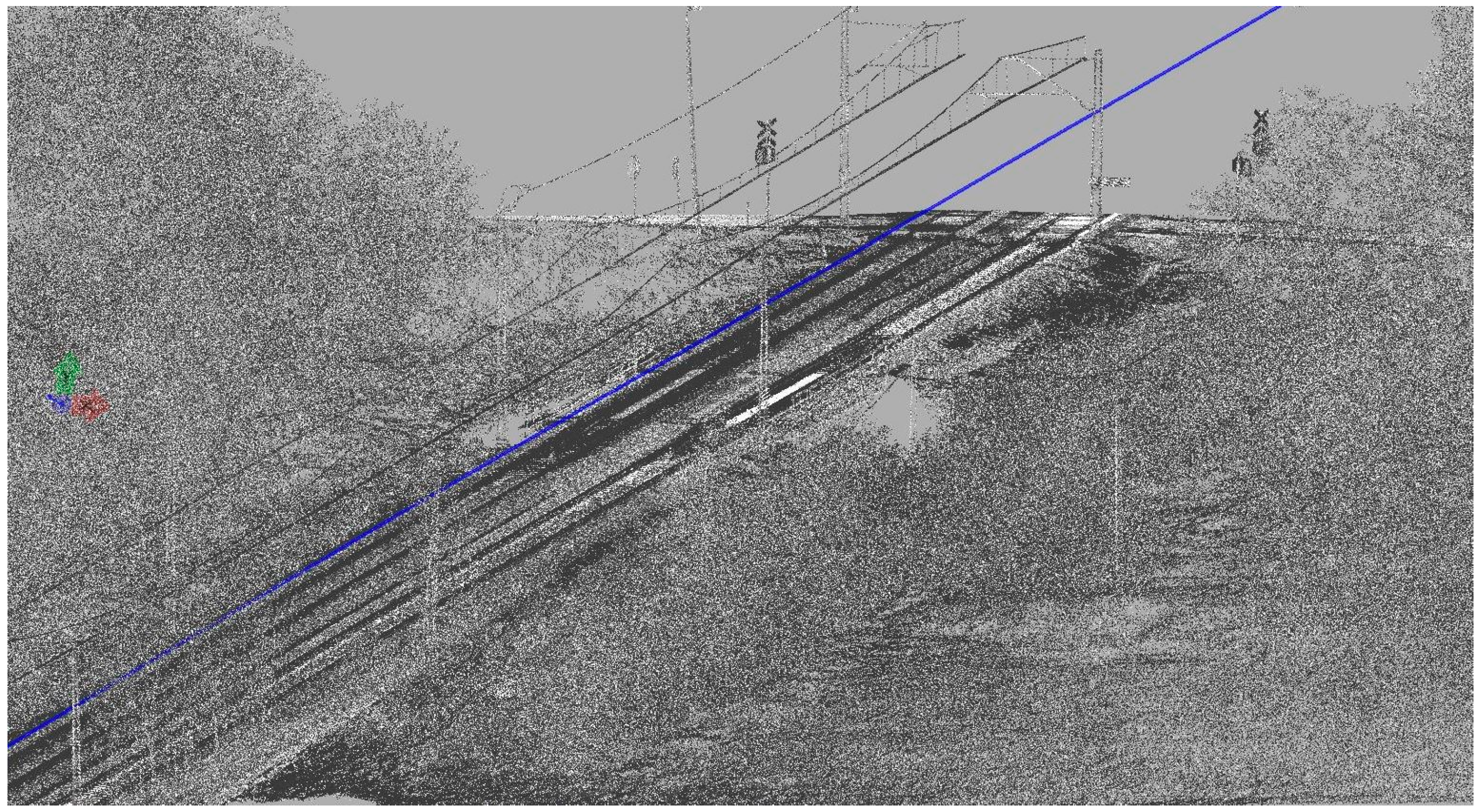
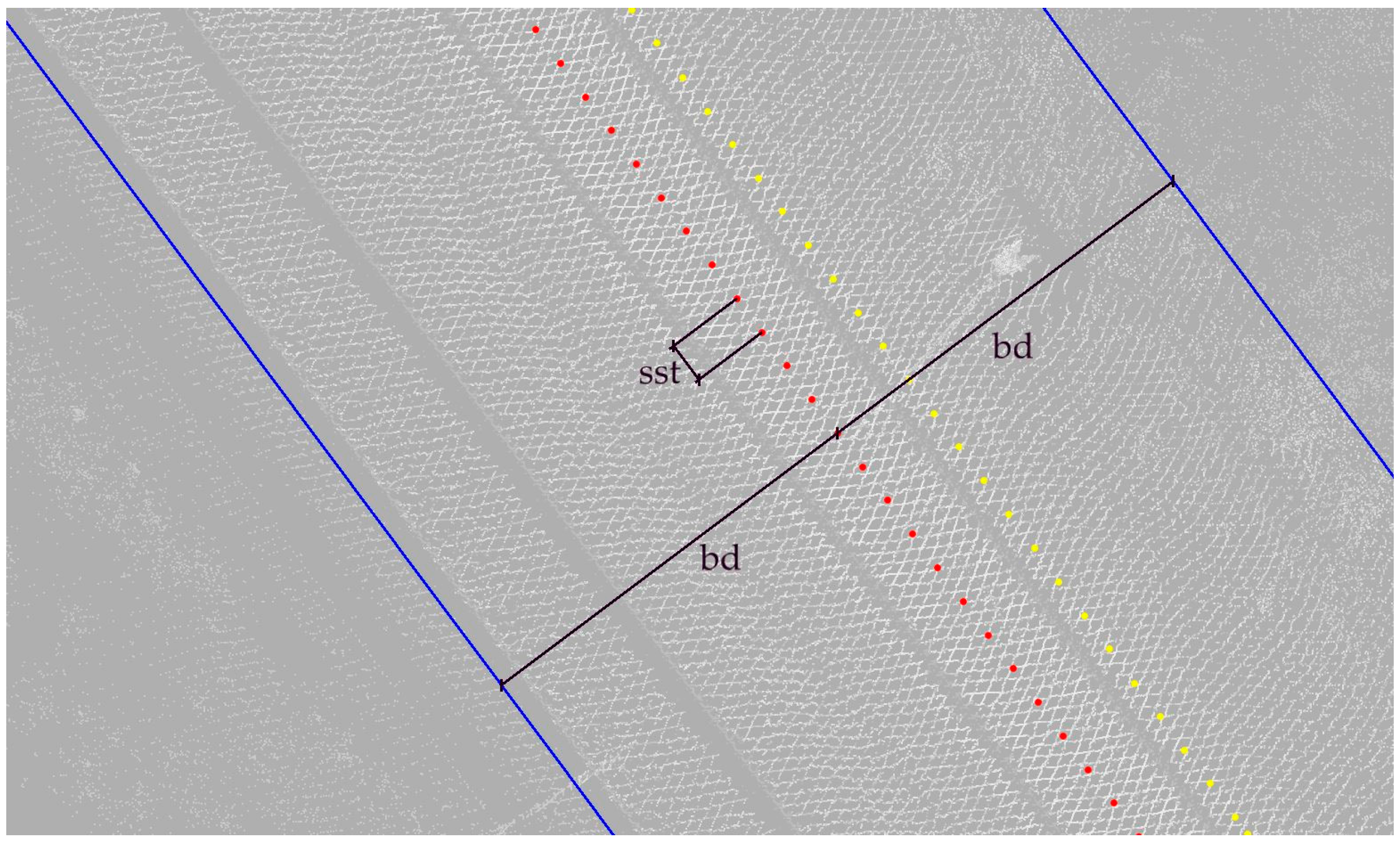
The second procedure limits the calculations of the later algorithm to points positioned up to a set distance horizontally from the registered trajectory: bd (Figure 7). It is necessary to set the limit according to regulations in force in the area where the survey took place. The limit should incorporate both railway clearance monitoring maximum distance, as well as the maximum distance from the track to one line support structure.

To keep order in point cloud processing and to be able to directly relate to specific parts of the data, an indexing system has been introduced. The processed point cloud is divided into sections along the route. Subsequent sections are given one, unchangeable index i {1, 2, 3...}. Each section is defined by its trajectory key point (KP_i), directional point (DP_i) and section depth (sd). Sets of consecutive key points (KP_i) and directional points (DP_i) are derived from the trajectory in established, even intervals, section steps (sst) (Figure 7). Key points belong directly to the trajectory. Each KP_i together with its corresponding DP_i forms a horizontal line perpendicular to the trajectory in said KP_i. The DP_i is positioned to the right of the trajectory, but its distance is of no importance and, as such, has been set to 1 m. Section i (S_i) is then a set of points lying within half a section depth from the vertical plane containing appropriate KP_i and DP_i.

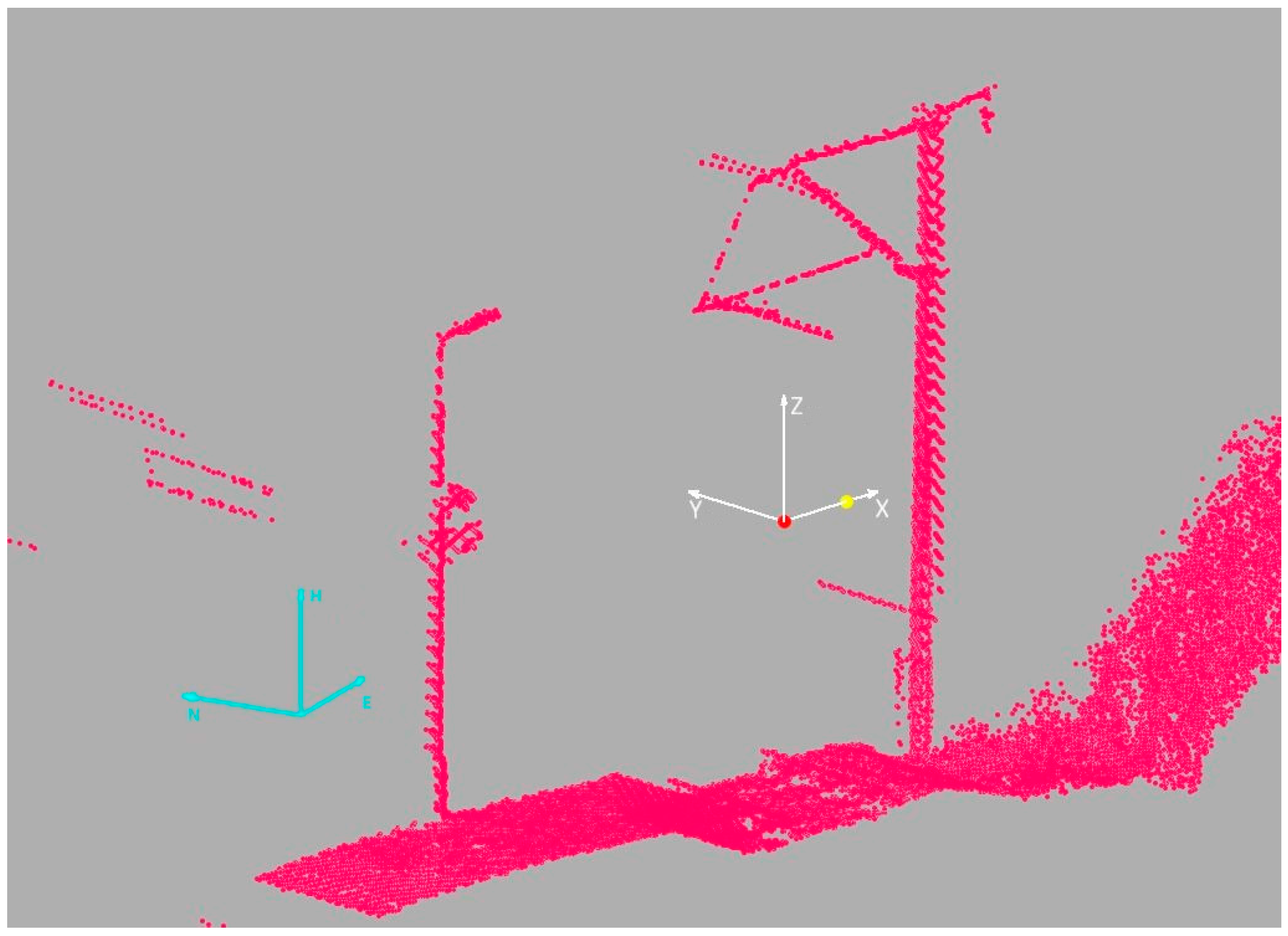
Two coordinate systems also need to be defined. The first coordinate system, the projected ENH (easting, northing, elevation) in which the MLS data are provided. The other is the local coordinate system X_iY_iZ_i, which is different for each section S(i) (Figure 8). Its origin lies in the KP_i; the X_i axis is directed towards the DP_i (off-track direction); the Y_i axis is perpendicular anti-clock-wise to the X_i axis (along the track direction); and the Z_i axis is parallel to the H axis of the projected ENH coordinate system. Units between the coordinate systems remain the same.

3.2.2. Initial Density Analysis

As previously explained, the design method uses geometric relationships in the MLS data. Point density is used to limit the search for support structures. A matrix is created with one column and rows corresponding to the index i. The value of the i-th cell is a number of points within an i-th section at a set distance from the trajectory both horizontally and vertically:

$${\mathrm{o}}_{\mathrm{i},1}=\#\mathrm{T}\left(\mathrm{i}\right)$$

(1)

where

$$\mathrm{T}\left(\mathrm{i}\right):= \left\{\mathrm{p}\left(\mathrm{X},\mathrm{Y},\mathrm{Z}\right)\in \mathrm{S}\left(\mathrm{i}\right):\mathrm{Z}\in \left[{\mathrm{h}}_{\mathrm{l}},{ \mathrm{h}}_{\mathrm{h}}\right] \wedge \mathrm{X}\in \left[-\mathrm{d},\mathrm{d}\right]\right\}$$

(2)

where, S(i), set of points belonging to section i; h_l, h_h, elevation distance limits; d, horizontal distance limits along the X axis.

Additionally, for each section, a region boundary is saved. Border vertices are calculated using the maximum values of the coordinates of the set of section points in the local 2D coordinate system, anchored in the trajectory key point and set in the section plane. Points lying within the calculated boundaries are assigned to the class catenary system. The lower left vertex (LL) is calculated:

$$\mathrm{LL}: = \left({\mathrm{X}}_{\mathrm{LL}},0,{\mathrm{Z}}_{\mathrm{LL}}\right)$$

(3)

where

• X_LL, lowest X coordinate value within points in the subset T,
• Z_LL, lowest Z coordinate value within points in the subset T.

Accordingly, the upper right vertex (UR):

$$\mathrm{UR}: = \left({\mathrm{X}}_{\mathrm{UR}},0,{\mathrm{Z}}_{\mathrm{UR}}\right)$$

(4)

where

• X_UR, highest X coordinate value within points in the subset T,
• Z_UR, highest Z coordinate value within points in the subset T.

The statistical parameters of the density matrix have been calculated to provide the information necessary to establish the correct binarization threshold. Firstly, the average number of points per section and, then, the population standard deviation are calculated.

$$\overline{\mathrm{o}} = \frac{{{\displaystyle \sum }}_{\mathrm{i}=1}^{\mathrm{n}}{\mathrm{o}}_{\mathrm{i},1}}{\mathrm{n}}$$

(5)

$$\mathsf{\sigma } = \pm \sqrt{\frac{{{\displaystyle \sum }}_{\mathrm{i}=1}^{\mathrm{n}}{\left({\mathrm{o}}_{\mathrm{i},1}-\overline{\mathrm{o}}\right)}^2}{\mathrm{n}}}$$

(6)

where

• n, number of sections in a point cloud.

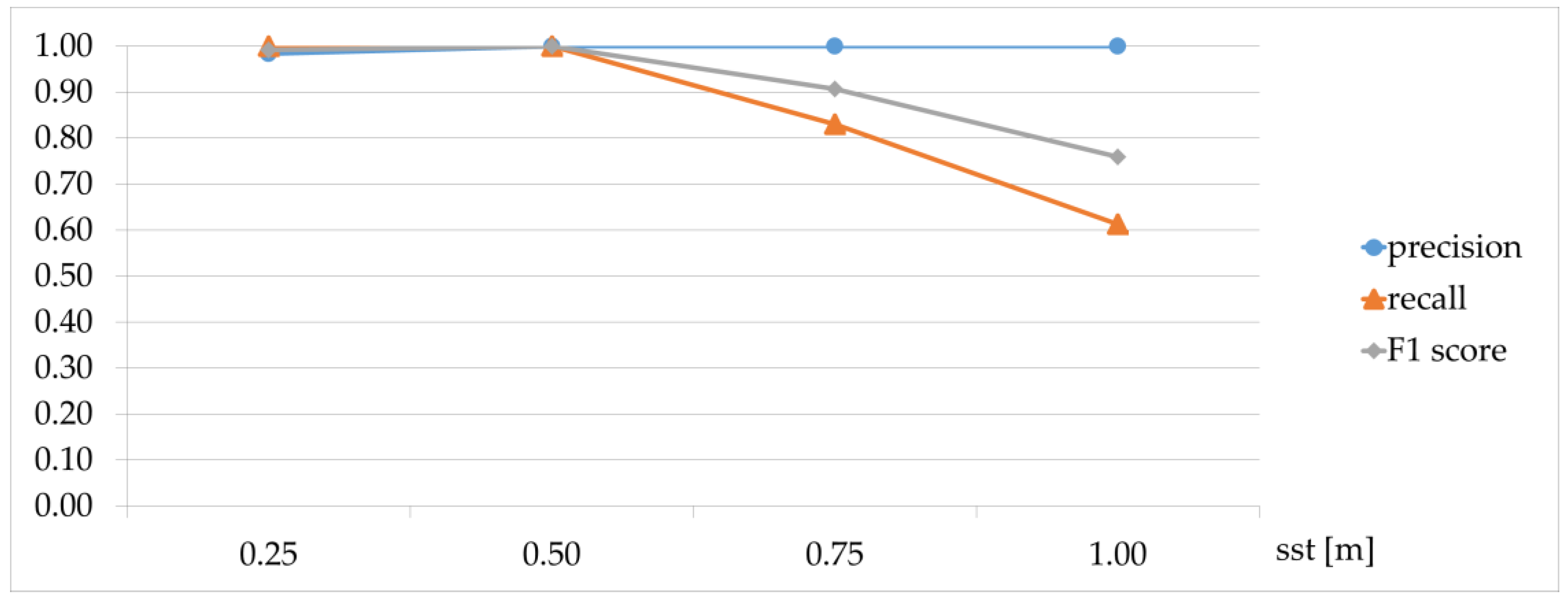
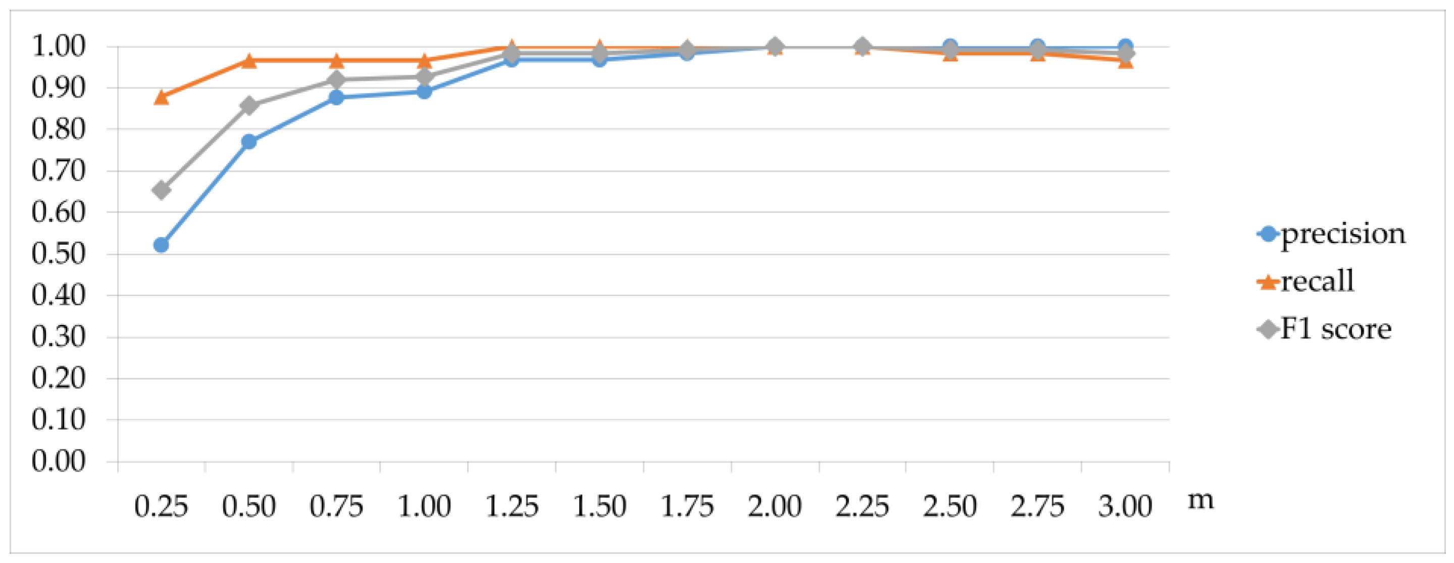
The matrix is then binarized with a threshold equal to the average number of points together with m times the population standard deviation [32]:

$${\mathrm{ob}}_{\mathrm{i},1} = \{\begin{array}{cc}1,& {\mathrm{o}}_{\mathrm{i},1}\ge \left(\overline{\mathrm{o}}+\mathrm{m}\mathsf{\sigma }\right)\\ 0,& \mathrm{in} \mathrm{other} \mathrm{cases}\end{array}$$

(7)

The value of the m parameter was determined during threshold sensitivity analysis in Section 5.1.

Then, the process, similar to morphological image processing, dilatation, is conducted to gather areas of interest lying in the near vicinity. A circle with a radius equal to 1 matrix unit has been used as a structuring element. Next, all existing area centers are found, and their index numbers (row numbers) are derived, to form a set of places of interest (W).

3.2.3. Support Structure Verification and Classification

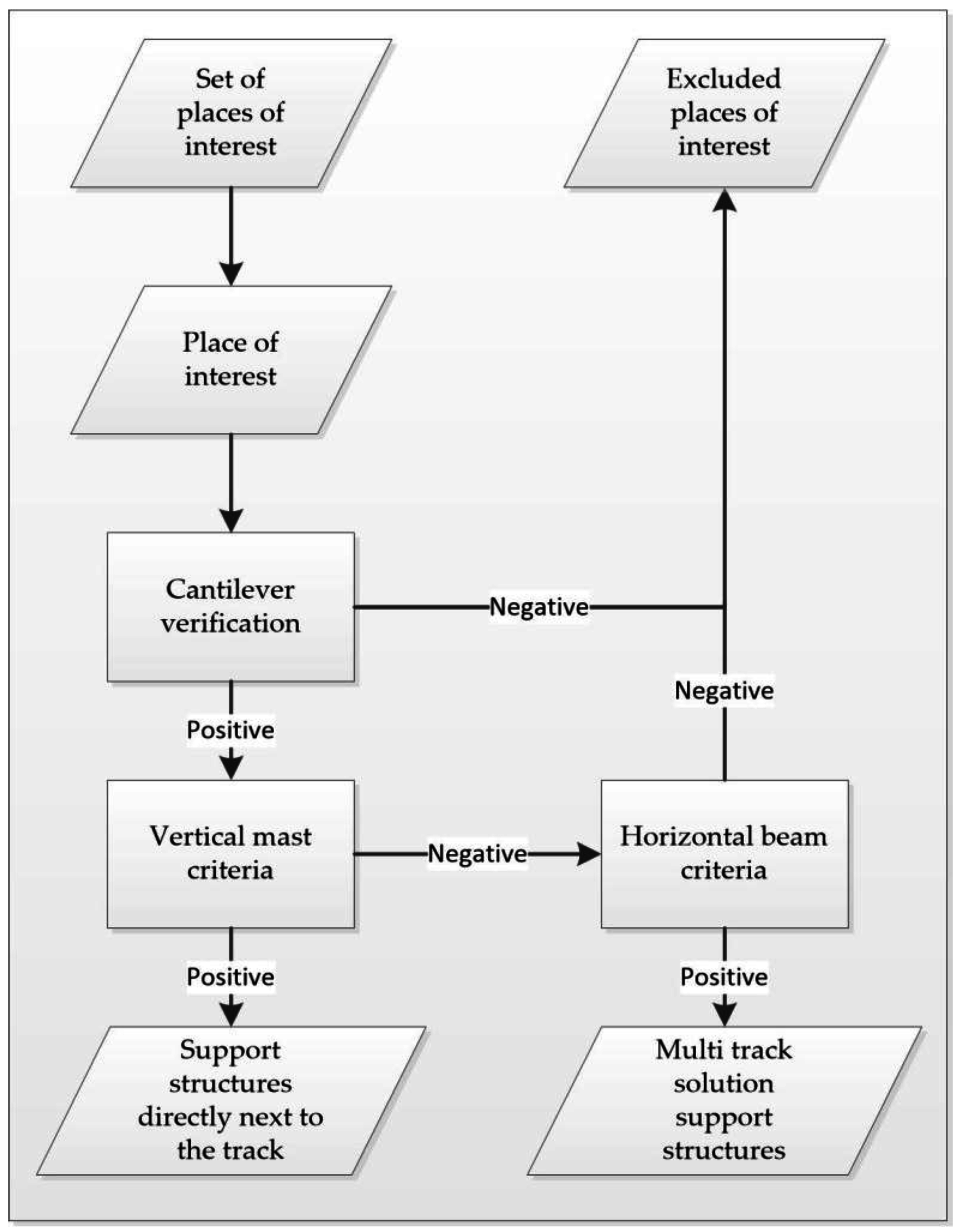
The verification process has a couple of consecutive steps. The simplified algorithm structure is presented in Figure 9.

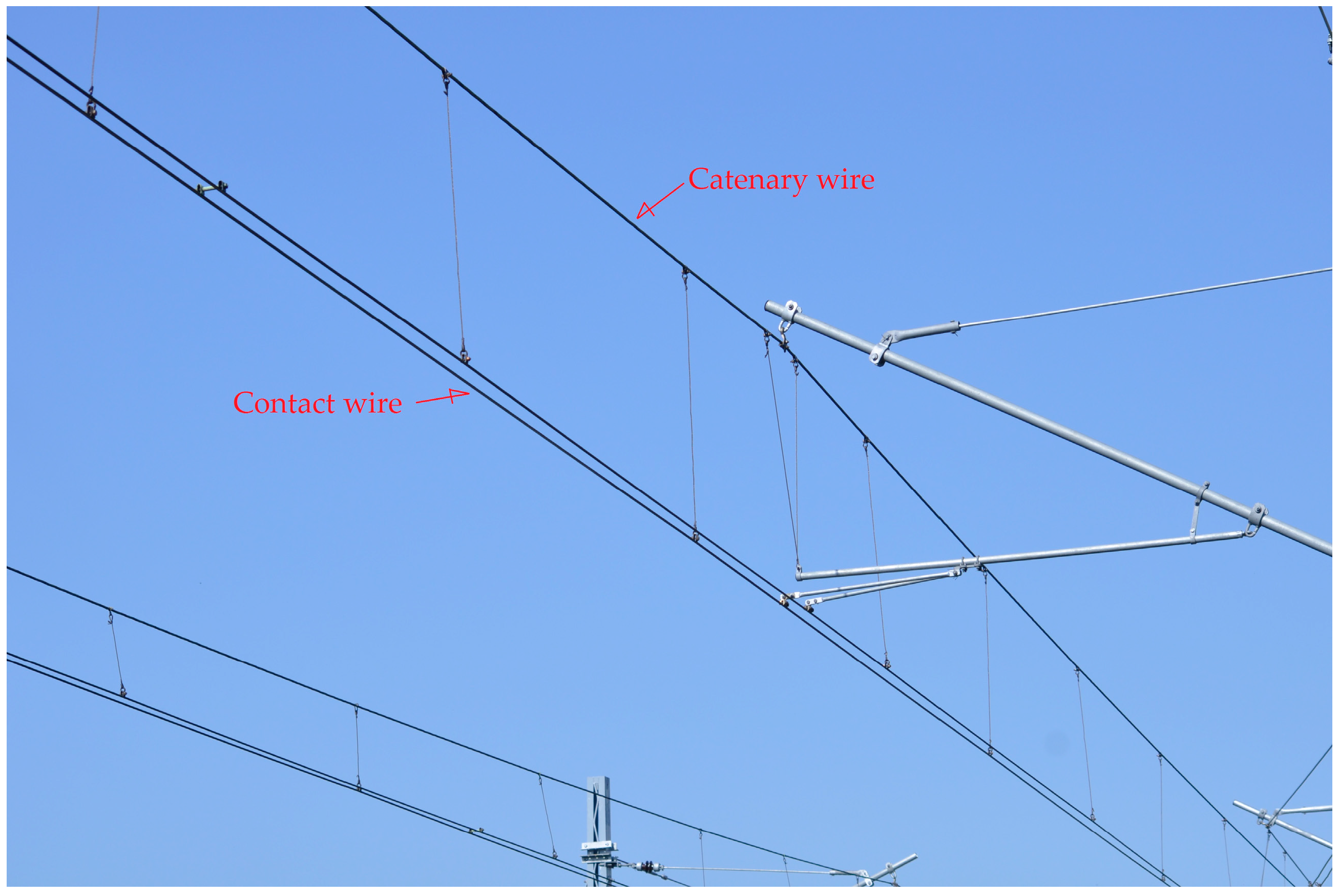
(i) Cantilever Criteria

A higher point density above the track can indicate not only the presence of cantilevers (Figure 10a), but also the joining of an additional track on turnouts/crossings (Figure 10b), double catenary wires at the ends of tensioning sections or vegetation growing too close to the catenary wires. Depending on the object causing the increase of point density, the points registered above the track projected on a horizontal plane will form a different pattern. As cantilevers are positioned almost perpendicular to the track, the pattern will resemble a cross. In other cases, there might be two lines meeting at an acute angle, turnouts, section tensioning ending, or the shapeless formation of points, vegetation.

To rule out false positives, each place of interest must be considered separately. Firstly, a set of points that should contain a catenary, together with the object causing the density increase, is selected based on the distance to the considered location. If a cantilever is present in a selected set of points, far more points should be registered on it than on catenary wires. All points are then projected onto a horizontal plane; the elevation coordinate is taken out of the equation; and then, a line is fitted to this set of points to determine the presence of cantilevers.

The RANSAC algorithm [42] has been used, as it performs well in very noisy environments. Through the years, this algorithm has been implemented in many point cloud-processing algorithms, including primitive shape detection [3] and roof detection [43]. RANSAC considers that the given data can be categorized into two sets, noise and model data. It then proceeds to fit the model to randomly-selected minimal sample data. The model that incorporates maximum data entities is chosen as the proper one. In the case of these calculations, cantilevers are the model (model distance r₁), and all other points are treated as noise.

If a determined line is almost perpendicular to the trajectory, a support structure can be verified; if not, the location is treated as a false positive. In the case of positive authentication, all model points are classified as the catenary system.

All verified places of interest are passed on for further categorization and support structure positioning.

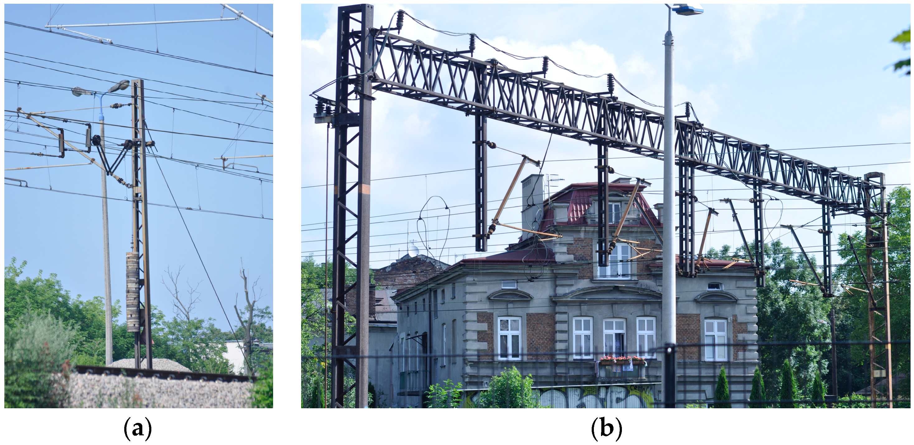
(ii) Vertical Mast and Horizontal Beam Criteria

Detected support structures are divided into two categories, traction poles and portal structures. The first category includes all construction where masts are located directly next to the applicable track, both single and multi-track solutions. The second includes all remaining portal structures.

The division is performed based on localizing a mast in close proximity to the measured track. Firstly, a set of points is selected, limited horizontally to s_h along the trajectory and ±s_z from the trajectory key point vertically. The area to the right and to the left side of the track is checked separately. There are four possible outcomes of said procedure.

• Number of points to the right exceeds set threshold and to the left does not.
• Number of points to the left exceeds set threshold and to the right does not.
• Number of points to the right and to the left exceed set threshold.
• Number of points to the right and to the left do not exceed set threshold.

The two first cases suggest the possibility of a mast next to the rail track. The third shows objects on both sides of the track, and the fourth implies a portal structure. As there are a great deal of different objects that might identify the existence of a significant number of points in the aforementioned subset, each case needs to be verified.

Case 1 and 2: A RANSAC algorithm is used to fit a line into a point selected by set horizontal and vertical limitations (model distance r₂). If the fitted line is almost vertical, the intersection of it and the terrain is calculated as the position of the traction pole. If the fitted line is not vertical, the place of interest is moved and is to be verified by the process for Case Scenario 4.

Case 3: To find a pole in this case, its separation from other objects is taken into consideration. Thus, on both sides, the RANSAC algorithm is used twice: once with a threshold distance r₂ and also with a threshold distance of 2r₂. Firstly, the vertical requirement is checked, and then, the number of model points between the 1st and 2nd set is compared. The pole is detected in the place where the difference between the number of set points in between iterations is smaller. The pole coordinates are calculated as in Cases 1 and 2. If none of the objects are established as vertical, the place of interest is moved and is then verified by the process for Case Scenario 4.

Case 4: There are no vertical pole-like objects next to the track. Therefore, either the support structure was verified incorrectly or this is a multi-track solution (portal structure) where the cantilever is secured to the structural beam above it. Again, RANSAC (threshold distance r₃) is used to fit the line to points above the catenary. If the line is perpendicular to the track and contains more points than the set threshold portal structure, it is verified, and its position trajectory key point is confirmed. In other cases, the point of interest is deleted from the checked set.

In all of the above cases, upon support structure verification, all RANSAC model points are classified as a catenary system. The minimal point count thresholds are set manually, according to point density.

3.2.4. Data Classification Clarification

As the process of classification has been simplified, not all points registered on the sought after infrastructure were found, and therefore, not all classified points were assigned correctly. The process of classification has been divided into two separate operations. The first considers detected support structures (i), the second catenary wires (ii).

(i) Support Structures

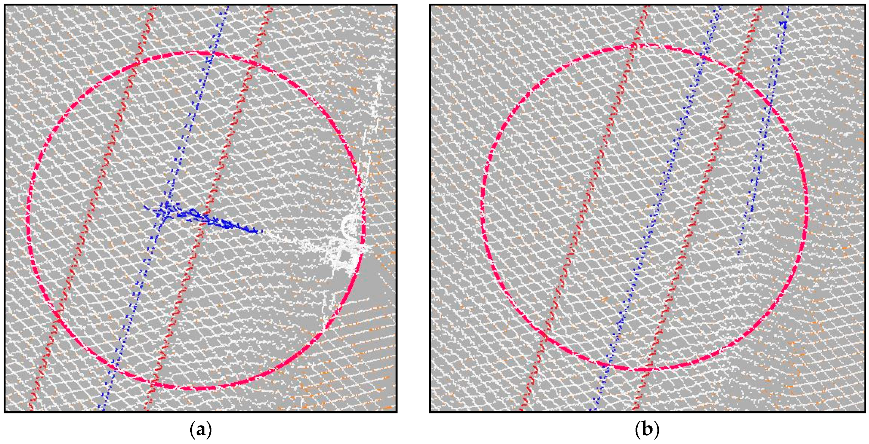
To refine the classification of support structures, a modification of the DBSCAN clustering algorithm was used. The DBSCAN algorithm, as published in [44], is used to perform data clustering of unorganized sets of data points. It can be applied to various sets of data, including point clouds [45]. It groups together points according to their neighborhood and distance. The algorithm proposes an iterative clustering method, which considers three types of points, core points, border points and outliers. Both core points and border points belong to the group. To assign unclassified points to the group, the point has to be within a set distance to one of the core points. It becomes a core point if there are more than a set number of group points in its neighborhood; otherwise, it becomes a border point.

DBSCAN’s simple principles make it easy to adapt it to this study. The algorithm has been modified to not detect a group of points, but being provided a set of points, among which some have been assigned to a certain group, to detect points among unassigned, which belong to said group. It has then been applied to each detected support structure in two separate calculations. The first considers all points from the middle (dm) vertically-wise and up and the second from the middle vertically-wise and down to stop the classification process from spreading along low vegetation and ground points. 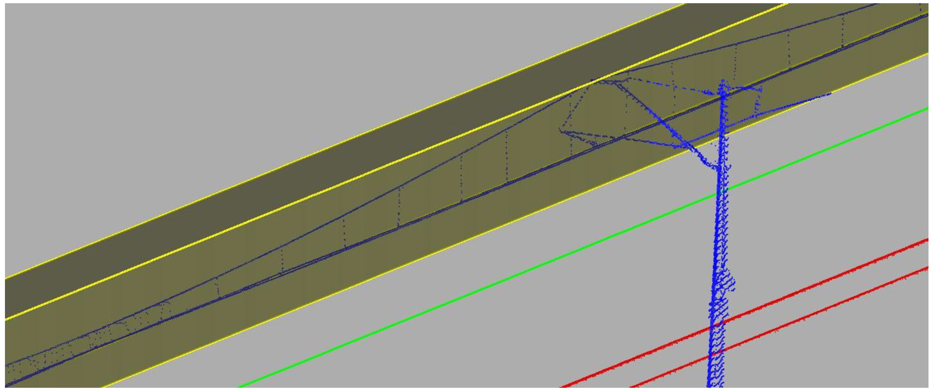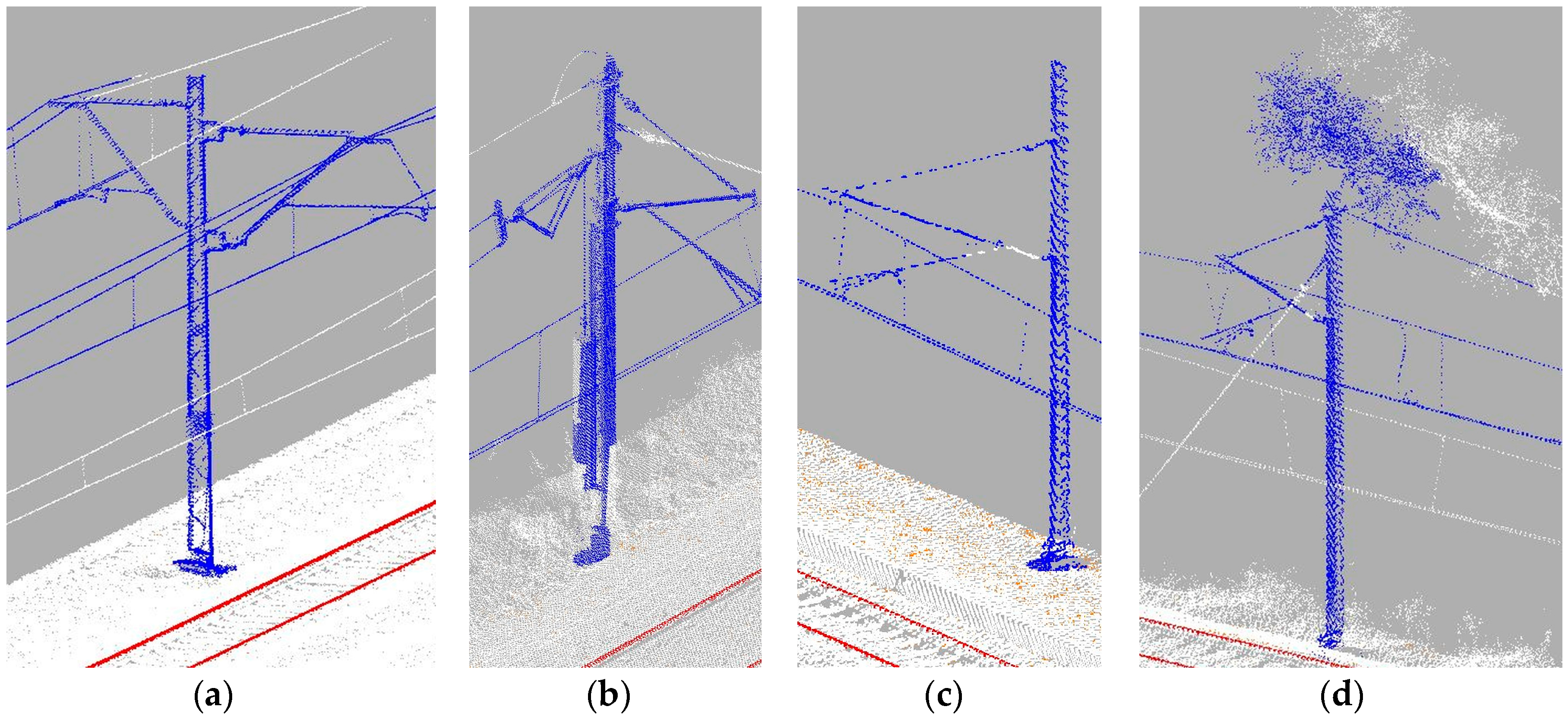Figure 11 presents detected support structures before and after the modified DBSCAN processing. Both distance and neighborhood thresholds have to be set according to the available data. DBSCAN parameters maximal distance (dd) and neighborhood count (nc) have to be set manually according to point density.

(ii) Catenary Wires

The goal of this step is to find points that do not belong to the catenary, but, due to simplified classification procedures, were included in this class. This includes greenery growing too close to the track, isolated noise points or other objects that might come into contact with the catenary. That also might include incorrectly excluded support structures. Boundaries determined during the initial density check procedure are considered (Section 3.2.2). In ideal circumstances, these boundaries would include only points registered on the catenary and, between the support structures, only the catenary cables. As the cables are being stretched, boundaries should linearly change between the consecutive sections.

To detect places of interest, the following procedure is implemented. Firstly, the whole analyzed railway line is divided into segments by all of the detected support structures. Then, the boundary diagonal is calculated for every section belonging to a considered segment. If, in between the consecutive sections, a discrepancy of the diagonal exceeds set threshold, c, then the region is evaluated again. There are two case scenarios where this can happen:

• an unidentified object too close to the catenary system,
• catenary cables heading towards tension poles or other tracks.

Determining each case is relatively easy. The cables heading towards tension poles or other tracks cause only one significant discrepancy between consecutive sections. In other case scenarios, there have to be at least two significant discrepancies nearby. In the event of the first case scenario, cables departing from the main thread, said cables are located by the RANSAC algorithm (model distance r₄). As it might be a set of cables instead of one thread, the search is conducted in sets of points projected onto a horizontal plane. The RANSAC model points are again classified as the catenary system. The second case scenario, for all of the sections where a significant discrepancy occurs, a new boundary is calculated. New boundary vertices are determined by the intersection of lines fitted to nearby boundary vertices and said section plane. All points excluded from the boundary in the newly-evaluated section are moved to an unassigned class. Additionally, the set of all corrected sections for the whole analyzed rail line is written to a separate file as objects that might jeopardize rail safety.

4. Datasets’ Description

Data used in this research have been obtained in the framework of a research project (No. 5.72.130.151) conducted by the AGH University for PKP Polskie Linie Kolejowe S.A. in Warsaw, Poland. Data were collected in 2011 and 2012 using RIEGL MMS VMX-250 and VMX-450 on a rail route between Cracow and Warsaw in Poland near the towns of Słomniki and Miechów. Both point clouds and trajectory coordinates were provided in the Polish National Coordinate System Poland CS2000 zone 7, which is a grid reference system using ENH coordinates. Collected data were divided into four datasets, according to the MMS system used, the date of survey and the direction of the survey (southbound/northbound) (

Table 1. Datasets used in the algorithm verification process.

Set	MLS System	Date of Measurement	No. of Points	Route Length (m)	Direction
I	RIEGL VMX-250	September 2011	780,468,277	31,711	northbound
II	RIEGL VMX-250	December 2012	609,748,916	20,065	northbound
III	RIEGL VMX-450	November 2012	677,251,514	18,938	southbound
IV	RIEGL VMX-450	November 2012	666,585,270	18,739	northbound

). Each set was then split into a number of point clouds.

The survey was conducted mostly on the same part of the rail route, though there are some exceptions. Figure 12 presents the extent of every survey mission. During surveys, the MMS were stabilized on the rail platforms differently (Figure 13), and so, all set distances had to be established individually. The test route length and location enabled the algorithm to be verified in various environments, the railway stations and areas between them, bends and straight sections. Within the test route, numerous types of support structures were found. They vary in terms of the type of construction, material and the level of degradation.

5. Results and Discussion

The assessment of the algorithm was conducted in three steps. Firstly, a threshold analysis was conducted to provide information as to how to set up correct levels. Then, a detection check (verification of the support structure positioning process) was carried out and, secondly, a classification check.

5.1. Threshold Analysis

The proposed method relies on a set of adopted thresholds. All of them can be divided into three categories:

• calculation parameters (Section 5.1.1),
• thresholds dependent on the geometry of the sought after objects (Section 5.1.2),
• thresholds dependent on the properties of MMS (Section 5.1.3).

Out of the four datasets, four point clouds form Set II, with a cumulative length of the route of approximately 2700 m, were chosen as the training data to set all thresholds and model all distances. Selected point clouds include both railway station and regular track, straight sections and bends. There are 59 support structures, both single solution and portal structures, registered within the chosen track. There is also a tensioning section and a turnout.

5.1.1. Calculation Parameters

Calculation parameters include basic thresholds and parameters, that is section step (sst), section depth (sd) and parameter m (Equation (11)). Section step and section depth have to have the same value to perform the calculation without loss of data.

To estimate thresholds’ optimal values, a sensitivity analysis was conducted. A two-stage approach was implemented for this purpose [46]. Firstly, thresholds were set intuitively (

Table 2. Adopted parameter sst and m values.

Parameter	Intuitive Value	Tested Values
sst	0.5	0.25, 0.50, 0.75, 1.00
m	2	0.25, 0.5, 0.75, 1.00, 1.25, 1.50, 1.75, 2.00, 2.25, 2.50, 2.75, 3.00

). Then, calculations were conducted with one threshold set and the other changing. As both thresholds are used within the initial density analysis (Section 3.2.2), precision, recall and F₁ score [47] were calculated for the case of the correct place of interest detection. The results for the analysis for the sst parameter are presented in

Table 3. Detection of the places of interest results according to various section step (sst) values.

sst Parameter (m)	Detected Places of Interest	True Positive	False Negative	False Positive	Precision	Recall	F1 Score
0.25	60	59	0	1	0.98	1.00	0.99
0.50	59	59	0	0	1.00	1.00	1.00
0.75	49	49	10	0	1.00	0.83	0.91
1.00	30	30	19	0	1.00	0.61	0.76

and Figure 14; the results for the analysis for the m parameter are presented in

Table 4. Detection of the places of interest results according to various m parameter values.

m Parameter	Detected Places of Interest	True Positive	False Negative	False Positive	Precision	Recall	F1 Score
0.25	98	51	7	47	0.52	0.88	0.65
0.50	74	57	2	17	0.77	0.97	0.86
0.75	65	57	2	8	0.88	0.97	0.92
1.00	64	57	2	7	0.89	0.97	0.93
1.25	61	59	0	2	0.97	1.00	0.98
1.50	61	59	0	2	0.97	1.00	0.98
1.75	60	59	0	1	0.98	1.00	0.99
2.00	59	59	0	0	1.00	1.00	1.00
2.25	59	59	0	0	1.00	1.00	1.00
2.50	58	58	1	0	1.00	0.98	0.99
2.75	58	58	1	0	1.00	0.98	0.99
3.00	57	57	2	0	1.00	0.97	0.98

and Figure 15.

Table 3 and Table 4 and Figure 14 and Figure 15 present the results of the calculations with the tested parameter values.

Both tested thresholds concern place of interest detection. Because of that, false positive cases’ impact is far less important than false negatives. Later calculations, among other things, are designed to exclude incorrectly chosen places of interest. Bearing that in mind, less false positive cases means less calculations and less time and computing power.

According to the results of sensitivity analysis, the section step was set to 0.5 m, and the m parameter was set to two.

5.1.2. Thresholds Dependent on the Geometry of the Sought after Objects

This category includes all of the set values and thresholds based on the properties of the catenary system. These thresholds are:

• bd, horizontal distance limiting the calculations of the algorithm,
• d, horizontal distance limits along X axis in initial density analysis,
• r₁, RANSAC model distance in the cantilever detection process,
• r₂, RANSAC model distance in the vertical pole detection process,
• r₃, RANSAC model distance in the horizontal beam detection process,
• r₄, RANSAC model distance in the catenary wire classification clarification process,
• s_h, s_z, distances used to determine the case in vertical and horizontal beam search,
• dm, elevation level dividing the support structure into two cases for DBSCAN processing,
• c, threshold for diagonal discrepancy in between consecutive sections’ catenary wire boundaries.

Railway embankments are highly regulated and standardized. Depending on the country or region, the parameters of the objects within the rail track and their relative position are arbitrarily set. Due to the constant monitoring, those parameters and relative positions will never change significantly. The parameters listed above were set in the algorithm according to Polish railway guidelines or cases observed within the dataset. The adopted thresholds values are:

• bd, 5 m, the railway clearance monitoring does not go beyond this limit, and one-line support structure masts are situated not further than 4.5 m from the track center,
• d, 1.5 m, set according to cantilever properties and the minimal distance from the rail axis to support structures,
• r₁, 0.1 m, the width of the cantilever does not exceed a couple of cm,
• r₂, 0.2 m, the diagonal of the thickest support structures does not exceed 0.4 m,
• r₃, 0.4 m, the diagonal of the horizontal beam in portal structures does not exceed 0.6 m,
• r₄, the model distance was set to 0.1 m to include cases of more and less tensioned wires,
• p_h, 1.5 m (3 sst), the value adopted according to possible deflection of the cantilever and section step value,
• p_z, 0.25 m from the trajectory, elevation below the catenary wires, but off the ground enough as not to include low vegetation,
• dm, h_l-0.5 m, elevation below the catenary wires, clearly dividing detected support structure into two point sets,
• c, 0.4 sst m, value adopted according to the section step and the angle of possible outgoing cables.

5.1.3. Thresholds Dependent on the Properties of MMS

There are two groups of thresholds dependent on the properties of MMS. The first group includes thresholds h_l, h_h, the trajectory to the catenary wires’ distances. To set the distance between MMS trajectory and catenary wires, two sample point cloud sections were chosen, one on a bend and one on a straight route, in all datasets. Adopted height differences according to the set are presented in

Table 5. Adopted height difference between the trajectory and catenary wires’ lower boundary (h_l) and upper boundary (h_h).

Set	hl	hh
I	1.85 m	4.85 m
II	1.90 m	4.90 m
III	1.60 m	4.60 m
IV	1.60 m	4.60 m

.

The second group includes DBSCAN set distance and neighborhood count (dd, nc). In this algorithm, for all sets, threshold dd was set to 0.1 m and nc to 20. The values were derived from the observation of a couple of randomly-chosen support structures. This value is the worst case scenario, but incorporates cases of both lattice and solid poles. The determination of these thresholds could be automated using the measurement of point density on the ground.

5.2. Support Structures Detection Check

All existing support structures were divided into three categories with regards to their detection: true positive, false positive and false negative. To qualify a support structure as detected, its location on the ground and type (single solution or multi-track solution) had to be written to the appropriate set. All entries in said sets were compared to manually-collected ground truth sets.

Table 6. Detection and positioning of support structure results. Support structures single solution, SS; multi-track solution, MTS.

Set	Existing		True Positive Detection		False Negative Detection		False Positive Detection
	SS	MTS	SS	MTS	SS	MTS	SS	MTS
I	575	24	546	24	29	0	1	2
II	357	11	352	11	5	0	0	0
III	356	7	351	7	5	0	0	0
IV	348	8	346	8	2	0	0	0

lists all results according to the dataset.

Table 7. Precision, recall and F₁ score according to dataset.

Set	Precision	Recall	F1 Score
I	0.9948	0.9516	0.9727
II	1.0000	0.9864	0.9932
III	1.0000	0.9862	0.9931
IV	1.0000	0.9944	0.9972

presents performance measures, precision, recall and F₁ score [47], which were calculated separately for each dataset.

All of the calculated performance measures are very high. The algorithm has proven to be both efficient and precise. It was able to detect over 97% of existing support structures, and false positives make up less than 0.2% of all detected objects.

There are a few factors contributing to the false negative detection cases. Mostly, the blame can be attributed to random sampling in the RANSAC algorithm. No matter how low the probability, it is still possible that during the sampling process, no points registered at a cantilever were taken into consideration. The probability of this further increases in places with double cables, as in tensioning sections. This can be eliminated if instead of random samples, all possible combinations are used in the sample stage of RANSAC, but the computational time required and the rather small amount of omitted support structures deem it, in the author’s opinion, as excessive. The other reason for false negative detection was also the extreme degradation of some support structures. For example, there was one case where another support structure was already placed next to a damaged pole (within 0.5 m); but both were registered, and as a consequence, neither was detected. All in all, every single undetected support structure was registered in a subset of objects lying too close to the track and, in the end, could be classified manually.

False positive detection was caused either by greenery growing too close to the track and, thus, causing false verification and detection or by the existence of additional cables. Only three cases of false positive detection were recorded.

5.3. Classification Check

The second step of the algorithm assessment included classification evaluation. Each detected support structure was checked for the completeness of classification and for the possible false classification of objects nearby. One thousand five hundred eight one out of 1645 detected poles and portal structures (96.11%) were classified correctly and completely (Figure 16a). The confusion matrix for the classification process (object level) is shown in

Table 8. Confusion matrix for the complete classification of detected support structures.

	Catenary Class	Other Class
Catenary Class	1581	56
Other Class	8	no data

.

Incorrect classification cases can be divided into one of three categories. Category I includes support structures with additional wire-stretchers at the end of the overhead contact line tensioning section (Figure 16b), 34 cases. Due to atypical support structure construction, DBSCAN processing might be done on an incomplete dataset. This consequently caused partial classification of masts. Category II incorporates all support structures whose cantilevers were constructed with thin steel cables, and due to their size, not many points were registered on its surface, 22 cases. Poor sampling resulted in the incorrect omission of said points by modified DBSCAN (Figure 16c). Category III considers all support structures that were classified together with adjoining greenery, eight cases (Figure 16d). Trees or shrubs growing too close to detected poles caused modified DBSCAN to falsely assign their points to the catenary class. All cases according to the datasets are presented in

Table 9. Incompletely- or incorrectly-classified support structures according to type of error.

	Classification
Set	Correct	Incorrect	Category I (%)	Category II (%)	Category III (%)
I	552	18	16.67	55.56	27.78
II	350	13	23.08	61.54	15.38
III	336	22	100.00	0.00	0.00
IV	343	11	54.55	36.36	9.09
sum	1581	64	53.12	34.38	12.50

.

All of the immediate contact wires were classified correctly; any problems that arose were due to additional wiring on turnouts or by the ends of the tensioning sections. Figure 17 presents a classified point cloud in the vicinity of turnouts.

In conclusion, the algorithm performed really well on all provided datasets. It did not fail to detect and correctly classify catenary systems regardless of the environment, complexity and degradation. Simple and obvious assumptions, that led to the creation of the algorithm, are the same for almost all overhead contact systems around the world. Contrary to previously-published research on the topic, all of the points registered on the catenary system were classified into one class. It is not enough for the automatic creation of 3D models, but it is more than enough for the purpose of railway gauge clearance monitoring. Furthermore, including this algorithm as a preparation step in more complex solutions could significantly reduce their calculations.

6. Conclusions

The test route included railway bridges, railway stations, turnouts, crossings, straight sections and bends. The created method utilized specific object properties and simple geometrical observations. Its simplicity and limited use to obvious and common properties made it possible to detect support structures regardless of the type of construction or degradation. Out of the total 1686 existing support structures, only 41 were not detected, which gives a success rate of over 97%. Additionally, only three non-existent support structures (false positives) were detected. In conclusion, the algorithm proved to be both reliable and efficient. The simplicity of the algorithm might enable it to work with any available MMS point cloud, but this hypothesis requires verification. There are a couple of drawbacks to this method that will be improved in future research. There are a few thresholds set manually, some of which relate to point cloud local density. They could easily be replaced with statistically-computed values according to local ground point density. Those that cannot be replaced are the geometrical distances and properties of specific objects. These need to be specified by the end user. Another problem is massive data management. The extremely large amounts of data provided by MMS need to be stored in such a way as to facilitate quick navigation and processing. This could be achieved with the available GIS tools. These tools are required in order to modify the algorithm into software. With further research, the authors are also planning to extend the algorithm to include neighboring tracks. It would require implementing rail detection, then railroad centerline determination and, finally, the incorporation of the rail axis instead of the trajectory in calculations.

References

1. Mongus, D.; Žalik, B. Parameter-free ground filtering of LiDAR data for automatic DTM generation. ISPRS J. Photogramm. Remote Sens. 2012, 67, 1–12. [Google Scholar] [CrossRef]
2. Meng, X.; Wang, L.; Silván-Cárdenas, J.L.; Currit, N. A multi-directional ground filtering algorithm for airborne LiDAR. ISPRS J. Photogramm. Remote Sens. 2009, 64, 117–124. [Google Scholar] [CrossRef]
3. Schnabel, R.; Wahl, R.; Klein, R. Efficient RANSAC for point-cloud shape detection. Comput. Graph. Forum 2007, 26, 214–226. [Google Scholar] [CrossRef]
4. Borrmann, D.; Elseberg, J.; Lingemann, K.; Nüchter, A. The 3D Hough Transform for plane detection in point clouds: A review and a new accumulator design. 3D Res. 2011, 2, 1330–1334. [Google Scholar] [CrossRef]
5. Rodríguez-Cuenca, B.; García-Cortés, S.; Ordóñez, C.; Alonso, M.C. Automatic detection and classification of pole-like objects in urban point cloud data using an anomaly detection algorithm. Remote Sens. 2015, 7, 12680–12703. [Google Scholar] [CrossRef]
6. Zhu, L.; Hyyppa, J. The use of airborne and mobile laser scanning for modeling railway environments in 3D. Remote Sens. 2014, 6, 3075–3100. [Google Scholar] [CrossRef]
7. Novak, K. Integration of a GPS-receiver and a stereo-vision system in a vehicle. Close-Range Photogramm. Meet. Mach. Vis. 1990, 1395, 16–23. [Google Scholar]
8. Guan, H.; Li, J.; Yu, Y.; Chapman, M.; Wang, H.; Wang, C.; Zhai, R. Iterative tensor voting for pavement crack extraction using mobile laser scanning data. IEEE Trans. Geosci. Remote Sens. 2015, 53, 1527–1537. [Google Scholar] [CrossRef]
9. Zhou, L.; Vosselman, G. Mapping curbstones in airborne and mobile laser scanning data. Int. J. Appl. Earth Obs. Geoinf. 2012, 18, 293–304. [Google Scholar] [CrossRef]
10. Golparvar-Fard, M.; Balali, V.; de la Garza, J.M. Segmentation and recognition of highway assets using image-based 3D point clouds and semantic Texton forests. J. Comput. Civ. Eng. 2012, 29. [Google Scholar] [CrossRef]
11. Manandahar, D.; Shibasaki, R. Auto-extraction of urban features from vehicle-borne laser data. In Proceedings of the Commission IV Symposium, Geospatial Theory, Processing and Applications, Ottawa, ON, Canada, 9–12 July 2002.
12. McElhinney, C.P.; Kumar, P.; Cahalane, C.; McCarthy, T. Initial results from European Road Safety Inspection (EURSI) mobile mapping project. In Proceedings of the ISPRS Commission V Technical Symposium, Newcastle, UK, 21–24 June 2010.
13. Pu, S.; Rutzinger, M.; Vosselman, G.; Elberink, S.O. Recognizing basic structures from mobile laser scanning data for road inventory studies. ISPRS J. Photogramm. Remote Sens. 2011, 66, S28–S39. [Google Scholar] [CrossRef]
14. Jaakkola, A.; Hyyppä, J.; Hyyppä, H.; Kukko, A. Retrieval Algorithms for road surface modelling using laser-based mobile mapping. Sensors 2008, 8, 5238–5249. [Google Scholar] [CrossRef]
15. Balali, V.; Golparvar-Fard, M. Recognition and localization of traffic signs via 3D image-based point cloud models. In Proceedings of the ASCE International Workshop on Computing in Civil Engineering, Austin, TX, USA, 21–23 June 2015.
16. Timofte, R.; Zimmermann, K.; Van Gool, L. Multi-view traffic sign detection, recognition, and 3D localisation. Mach. Vis. Appl. 2014, 25, 633–647. [Google Scholar] [CrossRef]
17. Gikas, V. Three-dimensional laser scanning for geometry documentation and construction management of highway tunnels during excavation. Sensors 2012, 12, 11249–11270. [Google Scholar] [CrossRef] [PubMed]
18. Oskouie, P.; Becerik-Gerber, B.; Soibelman, L. Automated measurement of highway retaining wall displacements using terrestrial laser scanners. Autom. Constr. 2016, 65, 86–101. [Google Scholar] [CrossRef]
19. Villarino, A.; Riveiro, B.; Martínez-Sánchez, J.; Gonzalez-Aguilera, D. Successful applications of geotechnologies for the evaluation of road infrastructures. Remote Sens. 2014, 6, 7800–7818. [Google Scholar] [CrossRef]
20. Markovic-Chenais, S. Trends in Rail Transport. In Proceedings of the Economic Commission for Europe, Inland Transport Committee, Working Party on Transport Trends and Economics, Geneva, Switzerland, 10–12 September 2013.
21. European Commission on Mobility and Transport. EU Transport in Figures—Statistical Pocketbook 2014; Publications Office of the European Union: Luxembourg City, Luxembourg, 2014. [Google Scholar]
22. Glaus, R. The Swiss Trolley—A Modular System for Track Surveying. Ph.D. Thesis, ETH Zurich – Swiss Federal Institue of Technology, Zürich, Switzerland, 2006. [Google Scholar]
23. Mikrut, S.; Kohut, P.; Pyka, K.; Tokarczyk, R.; Barszcz, T.; Uhl, T. Mobile laser scanning systems for measuring the clearance gauge of railways: State of play, testing and outlook. Sensors 2016, 16. [Google Scholar] [CrossRef] [PubMed]
24. Gikas, V.; Daskalakis, S. Determining rail track axis geometry using satellite and terrestrial geodetic data. Surv. Rev. 2008, 40, 392–405. [Google Scholar] [CrossRef]
25. Gikas, V. Geodetic survey and track recording vehicle data combined for the accurate setting out of rails on slab track. J. Spat. Sci. 2005, 5, 13–23. [Google Scholar] [CrossRef]
26. Wei, H.; Zhu, H.; Wang, Z.; Wu, W. Center line coordinates survey for existing railway by 3-D constraints method. Telkomnika 2013, 11, 2816–2821. [Google Scholar] [CrossRef]
27. Yang, B.; Fang, L.; Li, J. Semi-automated extraction and delineation of 3D roads of street scene from mobile laser scanning point clouds. ISPRS J. Photogramm. Remote Sens. 2013, 79, 80–93. [Google Scholar] [CrossRef]
28. Yu, C.; Zhang, D. Road curbs detection based on laser radar. In Proceedings of the IEEE 8th International Conference on Signal Processing, Beijing, China, 16–20 November 2006.
29. Hernandez, J.; Marcotegui, B. Filtering of artifacts and pavement segmentation from mobile lidar data. In The International Archives of the Photogrammetry, Remote Sensing and Spatial Information Sciences; ISPRS: Vienna, Austria, 2009; Volume XXXVIII, Part 3/W8; pp. 329–333. [Google Scholar]
30. Brenner, C. Extraction of features from mobile laser scanning data for future driver assistance systems. In Proceedings of the 12th Agile Conference, Hannover, Germany, 2–5 June 2009.
31. Lehtomäki, M.; Jaakkola, A.; Hyyppä, J.; Kukko, A.; Kaartinen, H. Detection of vertical pole-like objects in a road environment using vehicle-based laser scanning data. Remote Sens. 2010, 2, 641–664. [Google Scholar] [CrossRef]
32. Pastucha, E.; Słota, M. Automatic extraction of traction poles using mobile laser scanning data. Arch. Photogramm. Cartogr. Remote Sens. 2012, 24, 267–278. [Google Scholar]
33. Golovinskiy, A.; Kim, V.G.; Funkhouser, T. Shape-based recognition of 3D point clouds in urban environments. In Proceedings of the 12th International Conference on Computer Vision (ICCV09), Kyoto, Japan, 27 September–4 October 2009.
34. Arastounia, M. Automatic Classification of LiDAR Point Clouds in a Railway Environment. Master’s Thesis, University of Twente, Enschede, The Netherlands, 2012. [Google Scholar]
35. Beger, R.; Gedrange, C.; Hecht, R.; Neubert, M. Data fusion of extremely high resolution aerial imagery and LiDAR data for automated railroad centre line reconstruction. ISPRS J. Photogramm. Remote Sens. 2011, 66, S40–S51. [Google Scholar] [CrossRef]
36. Neubert, M.; Hecht, R.; Gedrange, C.; Trommler, M.; Herold, H.; Krüger, T. Extraction of railroad objects from very high resolution helicopterborne LiDAR and ortho-image data. Int. Arch. Photogramm. Remote Sens. Spat. Inf. Sci. 2008, 38, 25–30. [Google Scholar]
37. Yang, B.; Fang, L. Automated extraction of 3-D railway tracks from mobile laser scanning point clouds. IEEE J. Sel. Top. Appl. Earth Obs. Remote Sens. 2014, 7, 4750–4761. [Google Scholar] [CrossRef]
38. Elberink, S.O.; Khoshelham, K. Automatic extraction of railroad centerlines from mobile laser scanning data. Remote Sens. 2015, 7, 5565–5583. [Google Scholar] [CrossRef]
39. Arastounia, M. Automated recognition of railroad infrastructure in rural areas from LiDAR Data. Remote Sens. 2015, 7, 14916–14938. [Google Scholar] [CrossRef]
40. Jwa, Y.; Sohn, G.; Kim, H.B. Automatic 3D power line reconstruction using airborne LiDAR data. Int. Arch. Photogramm. Remote Sens. 2009, 38, 105–110. [Google Scholar]
41. Jwa, Y.; Sohn, G. A multi-level span analysis for improving 3D power-line reconstruction performance using airborne laser scanning data. Int. Arch. Photogramm. Remote Sens. Spat. Inf. Sci. 2010, 38, 97–102. [Google Scholar]
42. Fischler, M.A.; Bolles, R.C. Random sample consensus: A paradigm for model fitting with applications to image analysis and automated cartography. Commun. ACM 1981, 24, 381–395. [Google Scholar] [CrossRef]
43. Tarsha-Kurdi, F.; Landes, T.; Grussenmeyer, P. Hough-transform and extended ransac algorithms for automatic detection of 3D building roof planes from LiDAR data. In Proceedings of the ISPRS Workshop on Laser Scanning 2007 and SilviLaser 2007, Espoo, Finland, 12–14 September 2007.
44. Ester, M.; Kriegel, H.P.; Xu, X. A Density-Based Algorithm for Discovering Clusters in Large Spatial Databases with Noise; AAAI Press: Menlo Park, CA, USA, 1996. [Google Scholar]
45. Gong, J.; Caldas, C.H. Data processing for real-time construction site spatial modeling. Autom. Constr. 2008, 17, 526–535. [Google Scholar] [CrossRef]
46. Mongus, D.; Zalik, B. An efficient approach to 3D single tree-crown delineation in LiDAR data. ISPRS J. Photogramm. Remote Sens. 2015, 108, 219–233. [Google Scholar] [CrossRef]
47. Powers, D.M.W. Evaluation: From precision, recall and F-measure to ROC, informedness, markedness and correlation. J. Mach. Learn. Technol. 2011, 2, 37–63. [Google Scholar]
Figure 1. Point cloud collected by a mobile mapping system (MMS) on a rail. Points colored according to intensity; MMS trajectory in blue.
Remotesensing 08 00801 g001
Figure 2. Catenary cables.
Remotesensing 08 00801 g002
Figure 3. Catenary system support structures. Single solution (a) and multi-track solution, portal structure (b).
Remotesensing 08 00801 g003
Figure 4. Narrow corridor containing catenary wires against selected points from the MMS point cloud. Catenary system, blue; rails, red; trajectory, green.
Remotesensing 08 00801 g004
Figure 5. The simplified algorithm structure.
Remotesensing 08 00801 g005
Figure 6. Points belonging to the ground class. Example from the MLS point cloud classified in TerraScan software (version 016.003).
Remotesensing 08 00801 g006
Figure 7. Sample point cloud. In red trajectory key points (KP), in yellow directional points, in blue border of calculation area.
Remotesensing 08 00801 g007
Figure 8. Sample point cloud section. Easting, northing, elevation (ENH) coordinate system in teal, section local coordinate system in white, section key point in red, section directional point in yellow.
Remotesensing 08 00801 g008
Figure 9. Simplified structure of the verification process.
Remotesensing 08 00801 g009
Figure 10. Sample point clouds in the place of interest and near vicinity. Increase of density caused by cantilever (a) and additional track (b). Search area limited by pink circle, catenary system in blue, rails, red, remaining points in white.
Remotesensing 08 00801 g010
Figure 11. Detected support structure before (a) and after (b) submission to modified DBSCAN processing. Red, rails, catenary class, blue, unclassified points, white.
Remotesensing 08 00801 g011
Figure 12. Ranges of individual test routes.
Remotesensing 08 00801 g012
Figure 13. Models of mounting MMS on open rail cars used during surveys. Left RIEGL VMX-250 survey in 2011, center RIEGL VMX-250 survey in 2012, right VMX-450 survey in 2012.
Remotesensing 08 00801 g013
Figure 14. Precision, recall and F1 score values according to different section step (sst) values.
Remotesensing 08 00801 g014
Figure 15. Precision, recall and F1 score values according to different m parameter values.
Remotesensing 08 00801 g015
Figure 16. Detected and classified support structures: correct classification (a), support structure with additional wire stretchers (b) (Category I); support structure with cantilevers constructed with thin steel cables (c) (Category II); support structure with incorrectly-classified greenery (d) (Category III). Blue, catenary class, red, rail class, orange, ground class, white, remaining points.
Remotesensing 08 00801 g016
Figure 17. Part of the route including turnouts. Detected overhead contact system points in blue, rails in red, remaining points in white.
Remotesensing 08 00801 g017