Communication

A General-Purpose Spatial Survey Design for Collaborative Science and Monitoring of Global Environmental Change: The Global Grid

by
David M. Theobald
Conservation Science Partners, Fort Collins, CO 80524, USA
Submission received: 4 June 2016 / Revised: 18 September 2016 / Accepted: 26 September 2016 / Published: 30 September 2016
(This article belongs to the Special Issue Monitoring of Land Changes)

Abstract

:
Recent guidance on environmental modeling and global land-cover validation stresses the need for a probability-based design. Additionally, spatial balance has also been recommended as it ensures more efficient sampling, which is particularly relevant for understanding land use change. In this paper I describe a global sample design and database called the Global Grid (GG) that has both of these statistical characteristics, as well as being flexible, multi-scale, and globally comprehensive. The GG is intended to facilitate collaborative science and monitoring of land changes among local, regional, and national groups of scientists and citizens, and it is provided in a variety of open source formats to promote collaborative and citizen science. Since the GG sample grid is provided at multiple scales and is globally comprehensive, it provides a universal, readily-available sample. It also supports uneven probability sample designs through filtering sample locations by user-defined strata. The GG is not appropriate for use at locations above ±85° because the shape and topological distortion of quadrants becomes extreme near the poles. Additionally, the file sizes of the GG datasets are very large at fine scale (resolution ~600 m × 600 m) and require a 64-bit integer representation.

Graphical Abstract

1. Introduction

A number of comprehensive and long-term monitoring programs have been developed to provide a deeper understanding of the conditions and changes of human and natural systems. For example in the United States, the National Science Foundation created a network of Long-Term Ecological Research stations and, more recently, the National Ecological Observatory Network [1]. Progress has also been made in specifying rigorous methods to design monitoring programs. A monitoring design specifies the resource to be monitored, what will be measured, how it will be measured (i.e., the response design), where it will be monitored (i.e., the survey design), how frequently it will be monitored, and how measurements will be summarized [2]. In this paper I focus on survey design—often called sample design or spatial design [3]—and how best to generate a rigorous, useful, and flexible survey design that specifies where environmental data will be collected. Stehman [2] suggests that a good survey design should be probability-based; have a low and known estimated variance; be spatially-balanced, simple, and cost-effective; and have flexibility as a key characteristic because of real-world, practical challenges that environmental monitoring programs inevitably face [4]. Four aspects of developing a sample design for monitoring landscape change are discussed here: probability-based design, spatial balance, cartographic projections, and sampling intensity (i.e., frequency).
The need for a probability-based design was underscored in recent guidance on fundamental design principles for global land-cover validation [5,6], because it ensures rigorous statistical inference. Probability-based monitoring design is a key component to the US National Park Service’s Inventory and Monitoring Program [7,8]; the US Forest Service Forest Inventory Analysis [9], the US Natural Resource Conservation Service’s National Resource Inventory [10], and the US Geological Survey’s Land Cover Trends program [11]. The US Environmental Protection Agency’s Environmental Monitoring and Assessment Program was a seminal effort to develop a probability-based, comprehensive, multi-purpose sample design (EMAP [12,13]).
Building on experience gained from EMAP, Stevens and Olsen [14] developed a spatial-balanced sampling (SBS) approach called Generalized Random-Tessellation Stratified [15], and additional software programs have been subsequently developed [16,17]. SBS is a combination of simple random and systematic sampling, where samples are random, but also guaranteed to be distributed across space [3]. This leads to more efficient sampling, defined as providing more information per sample unit, because it ensures that every sample is distributed across the population (or domain) being sampled. This is a desirable characteristic of surveys and particularly relevant for understanding land use change [17,18].
The basis for the EMAP design was a uniform tessellation of hexagons resulting in points that are roughly 27.1 km apart on the Earth’s surface [19]. A uniform tessellation based on specialized, global projection systems was needed to minimize differences in the sampling unit areas to enable equal probability of resources being sampled [13,20,21,22,23]. The Global Land Cover 2000 reference data also used a probability-based and equal-area projection [24]. However, I depart from this recent work that has assumed the need for an equal-area projected coordinate system by generating a global survey design that employs geographic coordinates (latitude/longitude). Although it has been well established that moving pole-ward away from the equator leads to increasing distortion in area and shape [23], spherical geometry algorithms can be used that account for non-planar situations. Moreover, ensuring that units account for changing area can be accomplished by directly incorporating the area of the geographic units when calculating the probability of a location being selected (described in more detail below). Using grid cells specified by equal-angle latitude and longitude cells (e.g., 1° × 1°) has numerous practical advantages. Geographic coordinates are ideally suited for global representation because they are easy to understand, simple to map, avoid conceptual and computational difficulties with map projections, and software is readily available to manipulate these datasets.
A central purpose of environmental monitoring is to sample features from continuous populations distributed over space [25] so that features are counted or observed within a specified area. This emphasis on areal sampling is consistent with Holmes’ [26] distinction between location-based sampling using points vs. area-based sampling using areas that completely tessellate a domain, at some level of spatial precision. As a consequence of recognizing the importance of sampling an area rather than a dimensionless location, the key aspect of a global sample design is the ability to account for varying area size in the sampling units. Ecologists have long used areal plots: a 1 m2, modified-Whitaker plot [27]; the FIA plot [9]; the NRI plot primary sampling area and points [10], etc. Even real-world features that are conceptualized as a 1D feature, such as a stream network, are sampled on the ground as areal features [28].
A final aspect of sample design to discuss is related to sampling intensity. Since environmental systems are dynamic, long-term monitoring designs must be robust to potential changes in the sampling frame. For example, many natural resources of interest are changing as a consequence of land use change and to climate change impacts, such as sea level rise, shifting ecotones, and changing distributions of resources of interest. One approach to address this challenge has been through “over-sampling” SBS designs (also called a master sample [26,29]). This works by drawing additional samples (e.g., 10% or 20% additional points) to be used in case a site (or location) is rejected from the original sample because of physical inaccessibility or denied access by the land owner [30]. A powerful property of SBS designs is that these extra points in the master sample remain spatially balanced. This method is robust to situations where the resource of interest is not found at a given location (error of commission) or was found originally but, over time, no longer occurs there (sampling frame contracts). However, over-sampling is not robust to the situation where the initial sampling frame was imperfect so that it omitted legitimate resources (error of omission), nor if the sampling frame expands into other areas over time, nor if a stratum was incorrect. Over-sampling remains reliant on the proper specification of a static sampling frame.
Relatedly, integrated environmental monitoring design requires stronger coordination both within and between natural systems and human institutions. For example, there has been long standing recognition for the need to integrate across natural systems or resource types (e.g., terrestrial, aquatic, and atmospheric [31]). Since different resources often need to be characterized at different scales (or levels of precision), the sampling design must be hierarchical to allow nested designs at different scales [32]. As a result, a multi-resolution, hierarchal sample design has important benefits. This issue suggests that a more general sample design is needed, rather than one that is specifically tied to an individual resource type (e.g., forests rather than soil erosion). Perhaps an even more practical and immediate challenge is to integrate across institutional and administrative boundaries. That is, typically, a survey design is generated for a specific geographic area that corresponds usually to an institutional boundary (e.g., a country monitoring design occurs only within a given country, or a monitoring program that is conducted on certain land owner/manager types). However, if an adjacent institution or agency wishes to conduct monitoring that will be complementary, typically they must start from scratch. Occasionally the desire to complement an existing design with increased density of samples occurs, such as a watershed group within a state/province that wants to add extra locations.
Finally, there is an opportunity to gain from an emerging trend of decentralized data collection [33] through volunteered geographic information or “citizens as sensors” [34], or crowdsourcing [35]. It is increasingly easy to locate (through GPS), collect, integrate, and visualize environmental data (e.g., through Google Earth, Collect Earth, or GeoWiki; see [36]). Although recent work has addressed challenges to visualize these global datasets [37], it remains difficult to organize these often ad hoc data collection efforts. A number of efforts have used a simple systematic sampling generated by the intersections of latitudinal and longitudinal degrees, such as the Degree Confluence project [38], which attempts to provide a picture and field-based description of the latitude/longitudinal confluence at 1° intervals and will ultimately result in over 50,000 locations being catalogued (for lower than 70° latitude). This work is interesting but does not fulfill the probability-based requirement, nor can it be extended or the intensity increased easily, without doubling up by going to 0.5° confluences, which requires four times the intensity of data collection.
Given these challenges and opportunities, my goal in this paper is to describe a global sample design that supports regional to global-scale monitoring of environmental resources that is flexible, comprehensive, and general purpose. To accomplish this goal, I pursue three objectives: (a) review the survey design that is generated by a GIS-based tool called Reversed Random Quadrant-Recursive Raster (RRQRR; [4]); (b) describe a global survey design (Global Grid, GG) and dataset that employs a sample generated by RRQRR; and (c) provide a canned sampling design dataset called the GG in open source format at a variety of scales that can be readily incorporated into various software platforms.

2. Materials and Methods

To generate a general purpose spatial survey design for monitoring global environmental change, I first describe how a spatially-balanced sample design is generated using the Reversed Random Quadrant-Recursive Raster (RRQRR) algorithm and then discuss the generation of a specific application of RRQRR called the Global Grid (GG).

2.1. RRQRR Sample Design

The approach and algorithm to develop a SBS using the RRQRR approach is detailed elsewhere [4], so here I provide a brief review of key aspects of the method, and highlight the unique properties of survey designs generated by RRQRR in light of our goal to generate a global survey design. In brief, RRQRR sample designs are probability-based, spatially-balanced samples that have great flexibility. A sample design is generated by recursively subdividing an area into four units or cells (2 × 2) encoded with values 0, 1, 2, and 3. Rather than using a consistent ordering system, such as the Morton (or “z”) order, the ordering is randomized (actually permuted into one of 24 possible configurations). Each resulting cell has an independent probability (drawn from a uniform random distribution) of being selected, which is modified by the area of the resource in a cell being selected. RRQRR has been used to develop sample designs for a variety of purposes (e.g., [39,40,41,42,43]) including sampling within NEON domains. Software is readily available (see Supplementary Material) and a version of RRQRR is implemented in ArcGIS software [44]; see the example used by [41].
A first unique property of RRQRR is that rather than generating a sample of the complete list or sampling frame, it generates a full or “quasi-complete” sample of all possible locations for the entire geographic domain that contains the sampling frame. I call this a “quasi-complete” sample because although, theoretically, there are an infinite number of locations (if one assumes 0-dimensional sample locations or points), in practice there are a finite number of areas (cells) in a given tessellation. RRQRR uses a raster representation so the spatial precision is defined by the cell area, and the raster bounds is defined to be the minimum enclosing rectangle around the sampling frame of interest, typically buffered around the boundary by 10% or so. This quasi-complete sample provides nearly complete assurance that a sample will be robust to changes in a population frame. Note that “over-sampling” approaches (e.g., [30] provide some robustness only in the situation that additional samples are needed, but not if the dataset representing the frame is incorrect. For example, if a population frame representing streams is imperfect because a stream segment was subsequently found in the field, but not originally mapped, then, by definition, it cannot be over-sampled because there was no frame to sample from in the first place. However, because RRQRR provides a quasi-complete sample of the world, then all geographic features (to a given level of resolution) can be included in a probability-based sample design.
A second unique property of RRQRR design is that, in addition to the sequence raster dataset S, an additional raster layer (R) is provided at the same resolution that contains random values drawn from a uniform distribution (0, 1). R is used to “filter” locations based on a user-provided raster (A) that specifies the probability that a given location (raster cell) will be selected, relative to other locations to account for changes in the area of a resource being sampled at a given location. This maintains the requirement of probability-based sampling that every location has a known and non-zero probability of being sampled, and the probability of a cell being included in a sample is adjusted as a function of its area. If the size of the sample unit is relatively small (<1 km2) and the requirement for precision of estimates are relatively modest (i.e., within 0.01 km2), then area could be approximated by using planar-based area calculations, but adjusted for the decline in areas with increasing latitude as a function of cos(Lat). However, for higher precision, spherical geometry formulas should be used [45]). The practical advantages and simplicity of this system outweigh any minor limitations with shape, distance from centroid, and topology. Due to the extreme topological distortion as latitude approaches the poles, this approach is not appropriate for locations above ±85°.
For a global sample, the values in A would equal the ratio of the area of a cell divided by the maximum area of any cell (i.e., at the equator). Cells where R < A would be included in the sample. This accounts for the decreasing area of cells that when moving toward increasing latitudes away from the equator. For a regional or local sample, one could choose to use the maximum area of a cell within the local domain. To recognize situations where the resource of interest is variable in area within a cell (e.g., different lengths of streams), A could reflect not simply the area of the cell, but the area of the resource. Similarly, R can be compared to user-specified raster layer (I) containing inclusion probabilities to account for unequal probabilities to reflect strata, for example. That is, cells where R < I would be retained in the sample. The resulting sequence values in S may no longer be a sequential list of integers (e.g., 1, 2, 3, 4, 5…), and may have breaks in them (e.g., 1, 2, 4, 6, 7…), but the ordering of these sequence values remains important. This provides great flexibility to modifying and adjusting strata through the adjustment of the inclusion probabilities. Note that if unequal inclusion probabilities are used, then population estimates need to incorporate a weight w (typically w = 1/I).

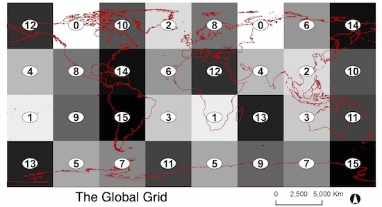
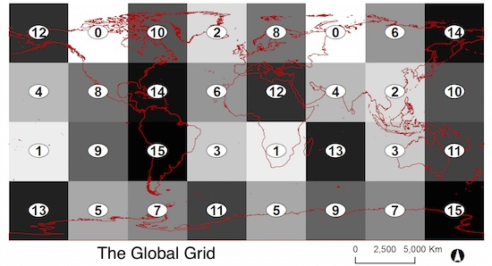
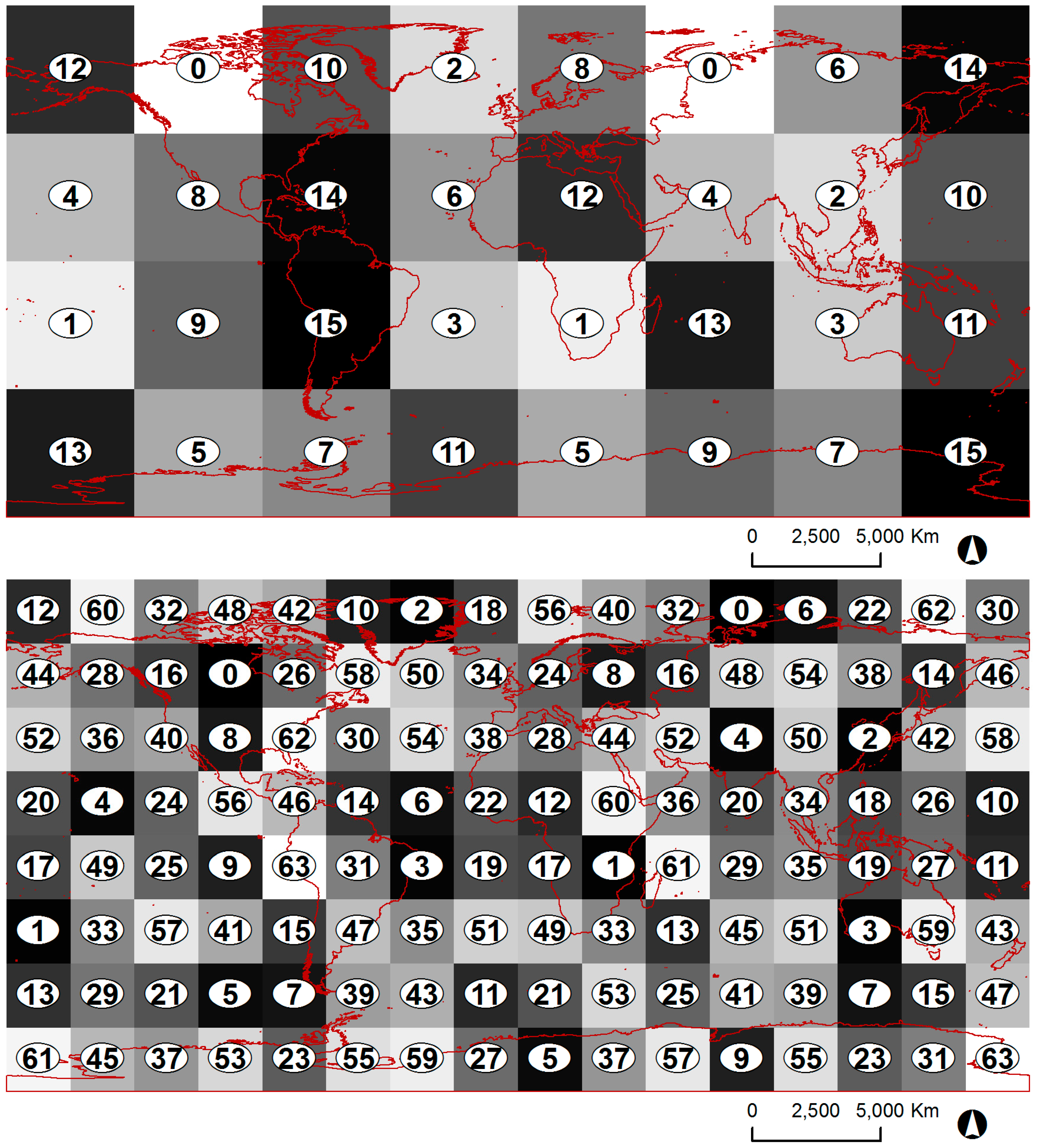
2.2. The Global Grid

To facilitate collaboration amongst researchers across different geographies, I provide a canned map or database of sample locations produced using RRQRR called the Global Grid (GG). The GG was generated by representing the globe using two cells that represent an expanse of 180° of longitude and latitude, placing the world into eastern (GGe) and western (GGw) hemispheres. Then, for each hemisphere, the first level (L = 1, GGw1, GGe1) is ordered 0, 1, 2, 3 (northwest, southwest, northeast, southeast). After the first level, each cell or quadrant is then recursively subdivided into fours and its sequence order is randomized. For instance, GGw2 and GGw2, cells are 45° on a side and the globe is represented by 32 cells (Figure 1). The GG can be further subdivided, generating nested hierarchical samples at each level (Table 1). At L = 14 sample cells are roughly 1.2 km on a side.
GG also provides the ability to modify the resulting sequence of sample locations by allowing users to adjust the relative inclusion probability based on the amount of a resource contained in a raster cell, rather than simply assuming that all (equal-area) cells contain the same amount of resource (e.g., [12,13]). Since cells (as quadrants) at different latitudes represent different surface areas, the relative inclusion probability needs to be adjusted by a weight w that ranges from 1.0 at the equator and approaches 0.0 at the poles. For example, for GG9, the area of cells at the equator is 1531.553 km2, which is used to normalize the w9 values from 1.0 at the equator to 0.003 near the poles. An extension of this concept can also incorporate the variability in the extent of a resource within a cell, e.g., the length of a stream resource represented by a cell depends on the location of the stream in the cell (going through the center or nipping a corner), as well as its sinuosity.
To account for the unequal surface area represented by each grid cell, a weight wL is computed for each cell that is a ratio of the area of a cell aL to the largest cell area in the sample, a × L, where wL = aL/a × L. If the weight is larger than a random value r (drawn from uniform distribution 0, 1), then the cell is removed from the resulting list (where cos(0.017453292520 × Lat) > r). For example, Figure 2 shows the first 1000 points of GG7. For samples with a global extent, this results in a removal of 34% of the points. A second issue is scale, that different types of resources of interest are appropriately sampled at different scales. Hierarchical nesting provides a multi-scalar, nested design such that the GG sequence value can be obtained at any level, and will be consistent between scales if a coarser/finer resolution is needed. If unequal inclusion probability is desired to have a higher density of sampling in some areas, then wL can be multiplied by the relative inclusion probability xL (0.1 to 1.0), where w’L = xLwL.
If the geographic domain over which an estimate is needed is not global, then the cells in the desired area can be extracted from GGL to make the resulting datasets smaller and easier to manipulate. This would be done typically to develop a specific design for a given resource type, for example, to target river networks [46]. Note that the sequence values in the resulting dataset will have large gaps in the sequence value (i.e., the will no longer be incremental), but the order of the sequence values remains important.

3. Results

The Global Grid (GG) dataset is available in a variety of spatial representations to make it readily useful and applied in various settings, including as raster, point, and area (i.e., quadrangles) spatial datasets. All data are generated in geographic coordinates using the WGS84 projection/datum. For each sample location, two attributes are provided: s, the sequence number that is specific to each level and hemisphere) and a random value r drawn from a uniform random distribution, which is used to compare against any inclusion probability weight during the filtering stage. In addition, the GG datasets are available as a .csv file (a well-known text format for ingesting into QGIS [47]), shapefile (for ingesting into Esri’s ArcGIS and other geographic information system software), and .kml for use in Google Earth (only the first 100,000 samples are provided because of display limitations). Note that these datasets are sorted ascending by sequence value, which makes it easy to use and select a subset of a specific number of samples (based on the ordered attribute FID). Raster data are also provided in a GeoTIFF format.

4. Discussion

The sample designs and datasets described here have numerous possible applications for environmental monitoring. For example, the RRQRR sampling design has been used to develop 6000 sample locations used to validate estimates of the degree of human modification [48]. Currently, the Global Grid is being used to develop a training and/or validation dataset of global human modification and land use/cover. The design takes advantage of using inclusion probabilities to sample at different intensities—in this case to have adequate sampling of more urbanized areas, which occupy ~5% of the terrestrial surface. To do this, I used “stable nightlights” for 2013 [49], calculated the mean brightness value within a radius of 10 kilometers, and then transformed the data using a natural log transform and rounded up to generate five classes (0–4) that correspond from rural to urban areas. I then generated an initial list of ~10,000 sample locations for terrestrial areas at level 14 (~1 km2) (Figure 3). The more heavily-developed portions of the world are readily visible as the sampling intensity was stratified to place random locations in more urbanized locations. The Global Land Use Emergent Database (GLUED; [50]) protocol is followed as the response design where 10 simple-random locations are placed within the ~1 km2 sample “chip”, and interpreters are encouraged at add up to 10 additional locations selected to represent rare features within the chip. This allows population estimates to be generated from the random datasets, while training data can also include the convenience sample points as well.
The Global Grid is designed to facilitate collaboration across various regions, by providing a single, stand-alone dataset that covers the entire globe at multiple resolutions. By providing both the sequence raster (S) and a random value raster (R), this database provides a platform for collaboration. For example, scientists who have expertise in a given region or domain could use the GG samples to interpret high-resolution aerial photography (or perhaps on the ground) to quantify land cover and land use types, degree of human modification, impervious surface, etc. Scientists in an adjacent region could then collect data using the same protocol and leverage the adjacent collected data because it comes from the same sample design so that spatial balance is maintained, thus ensuring the statistical rigor of a design-based sample. This same comprehensiveness also allows for easy expansion of a study area into adjacent areas that previously were not considered, perhaps to adjust to changing conditions of where a population is likely located, or simply as more study resources become available.
There are a few notable limitations of the GG. The surface area represented by each quadrant decreases as one moves pole-ward—which can be easily accounted for—but the shape and topological distortion becomes extreme near the poles. Hence, the GG is not appropriate for use at locations above ±85 degrees. Since the quadrants (cells) are predefined and the area of each quadrant at each subsequent level changes by a factor of four, it may not be appropriate for an application that requires a specific area tailored for a given purpose. Finally, the file sizes of the GG datasets are very large at fine resolution (levels > L10), particularly for >L15 which require a 64-bit integer representation.
General guidance for applying the Global Grid to a local or regional extent is as follows:
  • Level: determine the appropriate level (L) for the GGL sampling “chips” (see Table 1). Typically, GG14 is used for land use/cover validation (~1 km2). Note that GG sequence values are nested among scales, but each sequence value is particular to a given level.
  • Area: account for area differences in the amount of resource within each sample (quadrangle).
    2.1.
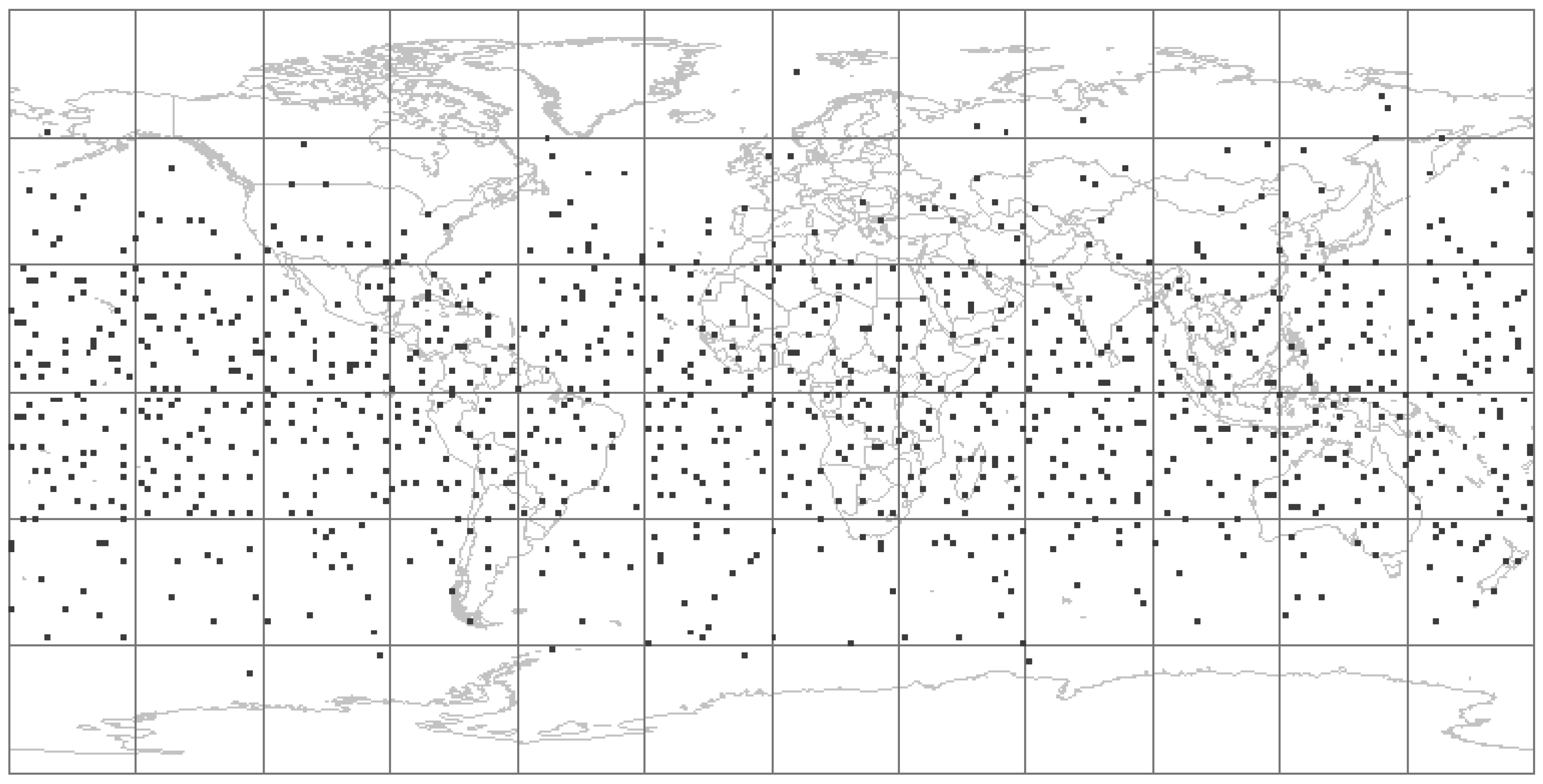
    Global: if a global sample is desired, then samples need to be removed relative to their area, which changes with the cosine of latitude. Query the GGL file to find samples where cos(Lat) > R, where R is a random value drawn from a uniform probability distribution.
    2.2.
    Regional: although less flexible and extendable, for some purposes a regional sample may be desired. In this case, the area of each sample polygon (quadrangle) can be calculated, and an area-based inclusion probability A can be calculated where A = Ai/Ax, where Ai is the area of sample i and Ax is the largest area within the regional sample (typically at the latitude closest to the equator). Query the GGL file to find samples where R < A.
    2.3.
    Variable area: frequently, the areal extent of a resource of interest to be sampled (e.g., a river or animal habitat) may vary within a given sample unit. To account for this, an exogenous raster layer can be provided by the user that calculates ai, the proportion of the resource found within cell i. Query the GGL file to find samples where (cos(Lat) × ai) > R.
  • Filtering: often additional filtering of samples is desired to adjust the sampling intensity to account for relatively rare features (e.g., using various strata) or to account for practical challenges in collecting response data at a given location (e.g., declining with further access from a road). If non-uniform inclusion probabilities are desired, then a separate spatial raster layer (I) of the same resolution as GGL, can be generated with values ranging from 0.0 to 1.0. Query the GGL file to find samples where (cos(Lat) × ai) > R and I > R.
  • Sequence: as standard practice, sequence values are sorted in ascending order (on the RRQRRL field). Capturing information typically proceeds in the order of the sequence values.

5. Conclusions

The Global Grid (GG) is database that provides a multi-scale, comprehensive spatial sampling design suitable for global environmental monitoring, which is generated using the Reversed Random Quadrant-Recursive Raster algorithm [4]. GG is a probability-based and spatially-balanced design, and because it is simple, flexible, and provides a quasi-complete sampling of the entire globe, it supports collaboration among disparate projects and scientists to align individual efforts so that their observations can be stitched together into a coherent whole. GG provides an unprecedented platform on which to conduct global monitoring while simultaneously facilitating coordination among regional and local scale efforts. GG is open source and freely available [51]. Possible future extensions of this work include providing more detailed resolution (levels 15 and beyond), making it available online through platforms, such as Google Earth, and interfacing with the Group on Earth Observations Biodiversity Observation Network Working Group 7: In Situ and Remote Sensing Integration.

Supplementary Materials

The following are available online at www.mdpi.com/2072-4292/8/10/813/s1. Datasets in KML format of Global Grid level 10 sample locations for terrestrial locations, with sampling intensity inversely proportional to the rural-to-urban gradient class 3.

Acknowledgments

This work was in part funded by NASA through cooperative agreement NNX15AD41G. I appreciate discussions with Barnett, D., Leinwand, I., Lewis, J., Norman, J., Urquhart, S., and Schweiger, W. and comments from Landau, V. on an earlier draft of this manuscript. I appreciate the useful comments of three reviewers that strengthened this paper.

Conflicts of Interest

The author declares no conflict of interest.

References

  1. Keller, M.; Schimel, D.S.; Hargrove, W.W.; Hoffman, F. A continental strategy for the National Ecological Observatory Network. Front. Ecol. Environ. 2008, 6, 282–284. [Google Scholar] [CrossRef]
  2. Stehman, S.V. Basic probability sampling designs for thematic map accuracy assessments. Int. J. Remote Sens. 1999, 20, 2423–2441. [Google Scholar] [CrossRef]
  3. Dobbie, M.J.; Henderson, B.L.; Stevens, D.L., Jr. Sparse sampling: Spatial design for monitoring stream networks. Stat. Surv. 2008, 2, 113–153. [Google Scholar] [CrossRef]
  4. Theobald, D.M.; Stevens, D.L., Jr.; White, D.; Urquhart, N.S.; Olsen, A.R.; Norman, J.B. Using GIS to generate spatially-balanced random survey designs for natural resource applications. Environ. Manag. 2007, 40, 134–146. [Google Scholar] [CrossRef] [PubMed]
  5. Olofsson, P.; Stehman, S.V.; Woodcock, C.E.; Sulla-Menashe, D.; Sibley, A.M.; Newell, J.D.; Friedl, M.A.; Herold, M. A global land-cover validation data set, part I: Fundamental design principles. Int. J. Remote Sens. 2012, 33, 5768–5788. [Google Scholar] [CrossRef]
  6. Tsendbazar, N.E.; de Bruin, S.; Herold, M. Assessing global land cover reference datasets for different user communities. ISPRS J. Photogramm. Remote Sens. 2015, 103, 93–114. [Google Scholar] [CrossRef]
  7. Oakley, K.L.; Thomas, L.P.; Fancy, S.G. Guidelines for long-term monitoring protocols. Wildl. Soc. Bull. 2003, 31, 1000–1003. [Google Scholar]
  8. Fancy, S.G.; Gross, J.E.; Carter, S.L. Monitoring the condition of natural resources in US National Parks. Environ. Monit. Assess. 2009, 151, 161–174. [Google Scholar] [CrossRef] [PubMed]
  9. Schreuder, H.T.; Czaplewski, R.L. Long-term strategy for the statistical design of a forest health monitoring system. Environ. Monit. Assess. 1992, 27, 81–94. [Google Scholar] [CrossRef] [PubMed]
  10. Nusser, S.M.; Breidt, F.J.; Fuller, W.A. Design and estimation for investigating the dynamics of natural resources. Ecol. Appl. 1998, 8, 234–245. [Google Scholar] [CrossRef]
  11. Stehman, S.V.; Sohl, T.L.; Loveland, T.R. Statistical sampling to characterize recent United States land-cover change. Remote Sens. Environ. 2003, 86, 517–529. [Google Scholar] [CrossRef]
  12. Overton, W.S. Probability sampling and population inference in monitoring programs. In Environmental Modeling with GIS; Goodchild, M.F., Parks, B.O., Stayert, L.T., Eds.; Oxford University Press: New York, NY, USA, 1993; pp. 470–480. [Google Scholar]
  13. White, D.; Kimerling, A.J.; Overton, W.S. Cartographic and geometric components of a global sampling design for environmental monitoring. Cartogr. Geogr. Inf. Syst. 1992, 19, 5–22. [Google Scholar] [CrossRef]
  14. Stevens, D.L., Jr.; Olsen, A.R. Spatially balanced sampling of natural resources. J. Am. Stat. Assoc. 2004, 99, 262–278. [Google Scholar] [CrossRef]
  15. Olsen, A.R. Software for R: Psurvey Analysis (3.3). 2016. Available online: https://cran.r-project.org/web/packages/spsurvey/index.html (accessed on 28 September 2016).
  16. Robertson, B.L.; Brown, J.A.; McDonald, T.; Jaksons, P. BAS: Balanced acceptance sampling of natural resources. Biometrics 2013, 69, 776–784. [Google Scholar] [CrossRef] [PubMed]
  17. Lister, T.W.; Lister, A.J.; Alexander, E. Land use change monitoring in Maryland using a probabilistic sample and rapid photointerpretation. Appl. Geogr. 2014, 51, 1–7. [Google Scholar] [CrossRef]
  18. Rindfuss, R.R.; Walsh, S.J.; Turner, B.L., II; Fox, J.; Mishra, V. Developing a science of land change: Challenges and methodological issues. Proc. Natl. Acad. Sci. USA 2004, 101, 13976–13981. [Google Scholar] [CrossRef] [PubMed]
  19. Overton, W.S.; White, D.; Stevens, D.L., Jr. Environmental Monitoring and Assessment Program: Design Report; EPA/600/3-91/053; US Environmental Protection Agency: Washington, DC, USA, 1990; p. 52.
  20. Wickman, F.E.; Elvers, E.; Edvarson, K. A system of domains for global sampling problems. Geogr. Ann. Ser. A 1974, 56, 201–212. [Google Scholar] [CrossRef]
  21. Dutton, G. Planetary modelling via hierarchical tessellation. In Proceedings of the Eleventh International Conference on Computer-Assisted Cartography (Auto-Carto 9); Anderson, E., Ed.; American Congress on Surveying and Mapping: Baltimore, MD, USA, 1989; pp. 462–471. [Google Scholar]
  22. Goodchild, M.F.; Shiren, Y. A hierarchical spatial data structure for global geographic information systems. Comput. Vis. Graph. Image Process. 1992, 54, 31–44. [Google Scholar] [CrossRef]
  23. Sahr, K.; White, D.; Kimerling, A.J. Geodesic discrete global grid systems. Cartogr. Geogr. Inf. Sci. 2003, 30, 121–134. [Google Scholar] [CrossRef]
  24. Mayaux, P.; Eva, H.; Gallego, J.; Strahler, A.H.; Herold, M.; Agrawal, S.; Naumov, S.; De Mirando, E.E.; Di Bella, C.M.; Ordoyne, C.; et al. Validation of the Global Land Cover 2000 map. IEEE Trans. Geosci. Remote Sens. 2006, 44, 1728–1739. [Google Scholar] [CrossRef]
  25. Stevens, D.L., Jr. Variable density grid-based sampling designs for continuous spatial populations. Environmetrics 1997, 8, 167–195. [Google Scholar] [CrossRef]
  26. Holmes, C. Problems in location sampling. Ann. Assoc. Am. Geogr. 1967, 57, 757–780. [Google Scholar] [CrossRef]
  27. Stohlgren, T.J.; Chong, G.W.; Kalkhan, M.A.; Schell, L.D. Multiscale sampling of plant diversity: Effects of minimum mapping unit size. Ecol. Appl. 1997, 7, 1064–1074. [Google Scholar] [CrossRef]
  28. US Environmental Protection Agency. Wadeable Streams Assessment; EPA 841-B-06-002; Office of Research and Development: Washington, DC, USA, 2006.
  29. King, A.J. The master sample of agriculture. J. Am. Stat. Assoc. 1945, 40, 38–45. [Google Scholar] [CrossRef]
  30. Larsen, D.P.; Olsen, A.R.; Stevens, D.L., Jr. Using a master sample to integrate stream monitoring programs. J. Agric. Biol. Environ. Stat. 2008, 13, 243–254. [Google Scholar] [CrossRef]
  31. National Research Council (NRC). Review of EPA’s Environmental Monitoring and Assessment Program: Overall Evaluation; National Academies Press: Washington, DC, USA, 1995. [Google Scholar]
  32. Schmeller, D.S.; Julliard, R.; Bellingham, P.J.; Böhm, M.; Brummitt, N.; Chiarucci, A.; Couvet, D.; Elmendorf, S.; Forsyth, D.M.; Moreno, J.G.; et al. Towards a global terrestrial species monitoring program. J. Nat. Conserv. 2015. [Google Scholar] [CrossRef]
  33. Becker, M.L.; Congalton, R.G.; Budd, R.; Fried, A. A GLOBE collaboration to develop land cover data collection and analysis protocols. J. Sci. Educ. Technol. 1998, 7, 85–96. [Google Scholar] [CrossRef]
  34. Goodchild, M.F. Citizens as sensors: The world of volunteered geography. GeoJournal 2007, 69, 211–221. [Google Scholar] [CrossRef]
  35. Lesiv, M.; Moltchanova, E.; Schepaschenko, D.; See, L.; Shvidenko, A.; Comber, A.; Fritz, S. Comparison of data fusion methods using crowdsourced data in creating a hybrid forest cover map. Remote Sens. 2016, 8, 261. [Google Scholar] [CrossRef]
  36. Fritz, S.; McCallum, I.; Schill, C.; Perger, C.; Grillmayer, R.; Achard, F.; Kraxner, F.; Obersteiner, M. Geo-Wiki.org: The use of crowdsourcing to improve global land cover. Remote Sens. 2009, 1, 345–354. [Google Scholar] [CrossRef]
  37. Dodge, M.; McDerby, M.; Turner, M. (Eds.) Geographic Visualization: Concepts, Tools and Applications; Wiley-Blackwell: Hoboken, NJ, USA, 2008; p. 348.
  38. The Degree Confluence Project. Available online: www.confluence.org (accessed on 27 September 2016).
  39. Tipton, H.C.; Dreitz, V.J.; Doherty, P.F. Occupancy of mountain plover and burrowing owl in Colorado. J. Wildl. Manag. 2008, 72, 1001–1006. [Google Scholar] [CrossRef]
  40. Pettebone, D.; Newman, P.; Theobald, D.M. A comparison of sampling designs for monitoring recreational trail impacts in Rocky Mountain National park. Environ. Manag. 2009, 43, 523–532. [Google Scholar] [CrossRef] [PubMed]
  41. Galway, L.P.; Bell, N.; Al Shatari, S.A.E.; Hagopian, A.; Burnham, G.; Flaxman, A.; Weiss, W.M.; Rajaratnam, J.; Takaro, T.K. A two-stage cluster sampling method using gridded population data, a GIS, and Google Earth imagery in a population-based mortality survey in Iraq. Int. J. Health Geogr. 2012, 11. [Google Scholar] [CrossRef] [PubMed]
  42. Marshall, K.N.; Cooper, D.J.; Hobbs, N.T. Interactions among herbivory, climate, topography and plant age shape riparian willow dynamic sin northern Yellowstone National Park, USA. J. Ecol. 2014. [Google Scholar] [CrossRef]
  43. Meunier, J.; Brown, P.M.; Romme, W.H. Tree recruitment in relation to climate and fire in northern Mexico. Ecology 2014, 95, 197–209. [Google Scholar] [CrossRef] [PubMed]
  44. ArcGIS Software, version 10.0; Esri: Redlands, CA, USA, 2015.
  45. De Smith, M.J.; Goodchild, M.F.; Longley, P.A. Geospatial Analysis: A Comprehensive Guide to Principles, Techniques and Software Tools, 2nd ed.; Troubador: Leicester, UK, 2008. [Google Scholar]
  46. Hall, R.K.; Olsen, A.; Stevens, D.L., Jr.; Rosenbaum, B.; Husby, P.; Wolinsky, G.A.; Heggem, D.T. EMAP design and river reach file 3 (RF3) as a sample frame in the Central Valley, California. Environ. Monit. Assess. 2000, 64, 69–80. [Google Scholar] [CrossRef]
  47. QGIS. Available online: www.qgis.org (accessed on 27 September 2016).
  48. Theobald, D.M. A general model to quantify ecological integrity for landscape assessments and US application. Landsc. Ecol. 2013. [Google Scholar] [CrossRef]
  49. Elvidge, C.D.; Baugh, K.E.; Dietz, J.B.; Bland, T.; Sutton, P.C.; Kroehl, H.W. Radiance calibration of DMSP-OLS low-light imaging data of human settlements. Remote Sens. Environ. 1999, 68, 77–88. [Google Scholar] [CrossRef]
  50. Global Land Use Emergent Database Group. Available online: https://groups.google.com/forum/?fromgroups#!forum/global-land-use-emergent-database (accessed on 27 September 2016).
  51. Theobald, D.M. Data from: A General-Purpose Spatial Survey Design for Collaborative Science and Monitoring of Global Environmental Change: The Global Grid. Dryad Digital Repository. Available online: datadryad.com (accessed on 27 September 2016).
Figure 1. The global sampling design strategy is hierarchical, multi-scalar, and comprehensive, which provides a tessellation of cells and a sampling order that maintains spatial balance. The first level (L) of the global grid (GG1) both the eastern and western hemisphere has cells of 90° on a side in the sequence 0, 1, 2, 3 (northwest, southwest, northeast, southeast). GG2 (top) has 16 cells of 45° on a side, while GG3 (bottom) has 32 cells of 22.5°. Note that the GGL+1 raster is nested within the GGL so that the sequence numbers follow.
Remotesensing 08 00813 g001
Figure 2. The first 1000 points of the Global Grid at level 7 (GG7), adjusted for global use.
Remotesensing 08 00813 g002
Figure 3. A global sample design of the Global Grid for terrestrial land use/cover, stratified on an urban to rural gradient generated from “nightlights” imagery from 2013.
Remotesensing 08 00813 g003
Table 1. The length of a side of a cell (in degrees and kilometers) and number of cells for each level of the Global Grid.
LevelDegreeskm (at Equator)No. of Cells
0180.00000 2
190.000009990.0008
245.000004995.00032
322.500002497.500128
411.250001248.750512
55.62500624.3752048
62.81250312.1888192
71.40625156.09432,768
80.7031378.047131,072
90.3515639.0235.24 × 105
100.1757819.5122.10 × 106
110.087899.7568.39 × 106
120.043954.8783.36 × 107
130.021972.4391.34 × 108
140.010991.2195.37 × 108
150.005490.6102.15 × 109
160.002750.3058.59 × 109
170.001370.1523.44 × 1011
180.000690.0761.37 × 1011
190.000340.0385.50 × 1011
200.000170.0192.20 × 1011
210.000090.0108.80 × 1011
220.000040.0053.52 × 1011
230.000020.0021.41 × 1014

