1. Introduction
Remote sensing and geographic information system (GIS) techniques are basic landslide analysis tools [
1] which give us the possibility of studying areas of different size and scale with adequate resolution and accuracy, as well as the ability to develop 3D and multi-temporal approaches. These techniques range from space remote sensing, in optical spectrum or Differential Synthetic Aperture Radar Interferometry (DInSAR) [
2,
3], to airborne photogrammetry and/or Light Detection and Ranging (LiDAR), which are frequently integrated. The selection of the appropriate technique depends on the scale and spatial resolution, the typology and evolution of the area and the availability of data.
In the case of medium to high resolution studies, with landslides of a diachronic evolution in which processes of reactivation separated in time take place [
4,
5], aerial photogrammetric techniques are very suitable and therefore their use is increasingly widespread [
5,
6,
7,
8,
9,
10,
11,
12,
13,
14,
15,
16,
17], sometimes combined with LiDAR [
5,
10,
12,
16] or global navigation satellite system (GNSS) techniques [
8]. In these studies, the image block orientation is based on conventional aerial triangulation techniques and bundle adjustment, using a reduced number of ground control points (GCP) measured with global navigation satellite system (GNSS) techniques [
18]. After image orientation, Digital Terrain Models (DTMs) or Digital Surface Models (DSMs, terrain plus the objects on it, both natural and artificial) are calculated using automatic matching techniques. Based on models from successive epochs, some quantitative approaches such as differential DSM/DTMs between campaigns, topographic profiles and volumetric calculations are addressed in practically all these studies; furthermore, in some of them, 3D displacement vectors are calculated [
6,
7,
8,
11,
15] and also observations for qualitative characterization of movements are made [
5,
6,
8,
10,
13,
14,
16].
On very high resolution studies, the last decade has seen an extensive use of Unmanned Aerial Vehicles (UAV), a technology in clear progression in many environmental applications. The use of UAVs or Remotely Piloted Aircraft Systems (RPAS), has recently been expanded to civil applications [
19,
20] including precision agriculture [
21,
22], civil protection and fires [
23], and more recently to engineering, environmental sciences and surveying [
24]. The present extensive use of UAVs has been stimulated by falling prices, the increasing miniaturization and improved performance of these systems, the recent developments with respect to GNSS and inertial systems, advances in autopilot guiding, etc. The current state of applicability is also due to the use of new algorithms in computer vision. Indeed, a new generation of low cost instruments and user-friendly photogrammetric software based on dense matching and Structure from Motion (SfM) approaches [
25,
26] has also contributed to this dramatic increase of UAV applications in environmental and Earth sciences.
In landslide research, different types of UAVs and methodologies have been used. Heavy equipment, usually fixed-wing drones [
27,
28,
29,
30,
31], but also helicopters, has been employed in high resolution studies. However, in most cases, light equipment such as multi-copters [
32,
33,
34,
35,
36,
37,
38,
39,
40,
41,
42,
43,
44,
45,
46] has been employed in very high resolution studies.
UAVs have been used in preliminary studies supporting other techniques such as remote sensing from satellites [
47,
48,
49], photogrammetry from historical flights [
27,
29,
31,
39,
40,
41] and airborne LiDAR [
31]. They have also been applied to inventory data collection studies by means of photo interpretation [
49,
50], change analysis [
27] and object-oriented analysis [
30], as well as the study of the effects of catastrophic events [
51]. In some cases, the aim of the study is the elaboration of susceptibility and stability maps [
33,
48,
49] and the assessment of the exposure of buildings or infrastructure to landslide risk [
33], but in other cases, the UAV techniques are integrated as subsystems for observation, material transport and rescue services in larger systems of quick response to emergency events [
29,
49,
52,
53].
Many approaches are based on the development of DSM/DTMs [
30,
31,
32,
33,
34,
35,
36,
37,
38,
39,
40,
41,
42,
43,
44,
45] and orthophotographs [
27,
28,
29,
30,
31,
32,
33,
34,
35,
36,
37,
38,
39,
40,
41,
42,
43,
44,
45]. In most cases, the starting point are flights oriented by aerial triangulation, based on ground control points (GCP) measured with GNSS [
30,
31,
32,
34,
35,
36,
37,
38,
39,
40,
41] or registered from previous photogrammetric [
29] or LiDAR models [
31,
39]. Structure from Motion (SfM) methods have also been tested [
26,
34,
35,
36,
37,
38,
39,
40,
41,
43]. While direct orientation from in-flight parameters (GNSS/INS) is routinely used in conventional aerial photogrammetry, such direct orientation techniques are not usually possible with present micro-UAVs when absolute orientation accuracy is a critical factor, although some experiments for direct orientation without GCP have also been undertaken [
26,
29,
46].
DTMs or, alternatively, DSMs are frequently used to obtain differential models for estimating the vertical displacements of the terrain surface [
30,
31,
34,
35,
36,
37,
38,
39,
40,
41,
45] and for volumetric calculations and profiles [
31]. Although DSMs introduce errors and uncertainties in terrain surface calculations, most authors use these models due to the difficulties in obtaining true DTMs from photogrammetric point clouds [
34,
35,
36,
37,
38,
39,
40,
41,
45], as in areas covered by dense vegetation. In other cases, the analysis of these models of very high resolution allows the automatic detection of scarps and other features of landslides [
43].
Orthophotographs—besides being used for landslide inventories, as in the aforementioned studies—allow the calculation of the horizontal displacements between significant points with great accuracy, given their high resolution [
30,
34,
35,
36,
39,
40,
41,
45]. In some studies, methods and algorithms for the automatic detection of movements of the terrain surface from the orthoimages have been proposed, as well as techniques of image co-registration [
30,
37,
38,
42]. Finally, some authors have used orthoimages for textural analysis of the fissures formed in the landslides [
36] and to determine vegetation indices such as GVI (Green Vegetation Index) for purposes of land classification or landslide inventory [
27,
30].
Moreover, when the measurement and monitoring of terrain deformation is the aim, analyses of the positional accuracy of the results have to be conducted. These studies can be carried out by means of error analysis of the GCPs (error propagation, distribution of points, field GNSS measurements, etc.) as well as the analysis of the resultant products such as DSM/DTMs or orthophotographs [
26,
28,
31,
32,
34,
41,
42,
45]. Generally, satisfactory results can be achieved, similar to those calculated with conventional aerial photogrammetry [
29,
44].
This paper deals with the use of UAV techniques for very high accuracy and resolution field data collection. Present UAVs allow fast, low cost and effective data acquisition. The study case is a multi-temporal analysis of an earth flow affecting an olive grove. Autopilot guiding missions allowed the acquisition of blocks of high overlapping stereo-models, which led to the detailed observation and mapping of terrain features. Furthermore, analysis from DSMs and orthophotographs could be carried out by comparing surfaces (differential DSMs) or measuring displacements between points. Given the difficulties of automatic identification and matching of points between multi-temporal images due to changes in vegetation, sun illumination and the landslide movement itself, the points were selected manually, but an approach was also tested for the semi-automatic calculation of displacements of the olive trees that cover most of the study area.
2. Study Area and Landslides
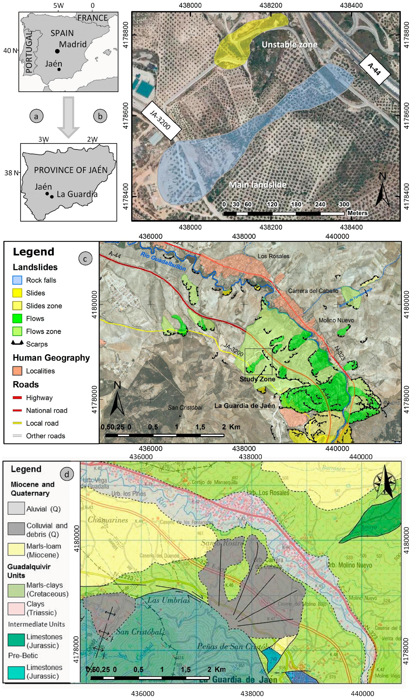
The area is located in an olive grove on a hillslope with a moderate gradient of 15% (5° to 20°) above the A-44 highway in La Guardia de Jaén, Southern Spain (
Figure 1a,b). In this area there are many landslide indications [
54], most of them corresponding to mud or earth flows [
55,
56], such as the study case of this paper, although slide-type movements have also been identified (
Figure 1c). Some of these have been studied by means of photogrammetric and LiDAR techniques [
57], but also with UAVs [
39,
40,
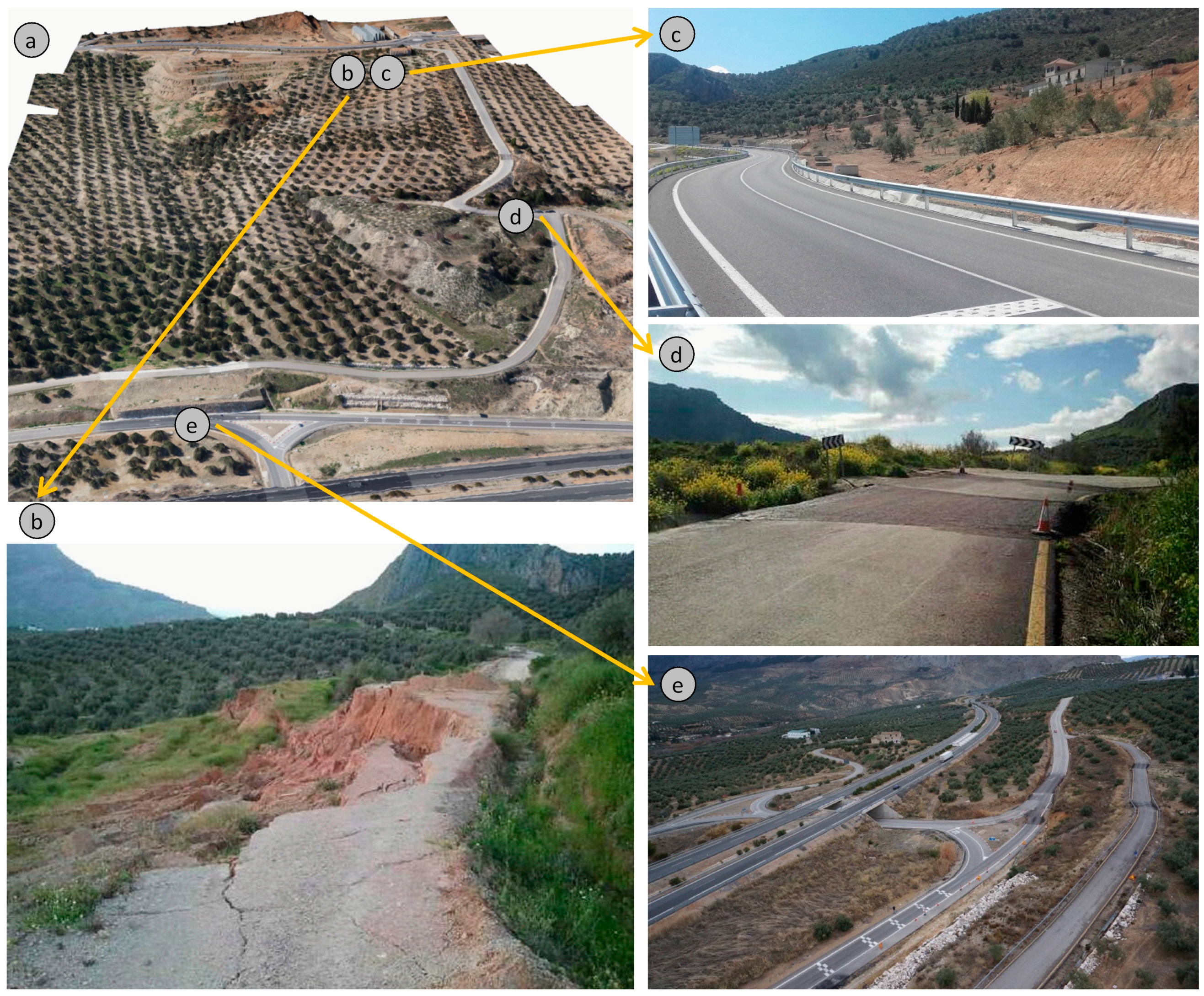
41]. The study movement occurred as a result of the heavy rains of winter 2012–2013, and had an approximate extension of 500 m length, 50–150 m width and a height difference of 80 m. The landslide seriously affected the roads in the area (
Figure 1c and
Figure 2).
The study area is located on the geological Guadalquivir Units [
58] (
Figure 1d), a set of materials with a complex structure and diverse lithology, in which the following formations predominate: Triassic evaporites and shales, Cretaceous-Paleogene marls and clays (from the Subbetic Units), and Miocene loamy-clay sediments belonging to the Guadalquivir basin. In this area, the Guadalquivir Units are overthrusted by Intermediate Betic Units represented by thick stratigraphic successions of folded Middle Jurassic limestones [
59,
60], which form a prominent relief. This thrust is affected by normal faults with a NNW-SSE direction. Both types of tectonic structures present geomorphological and seismic evidence of recent activity [
61,
62], which may be related to the regional uplift and subsequent slope instability processes. The contact is dotted with small alluvial fans, thick piedmont deposits and travertines. Travertines are associated with springs at the foot of the Jurassic limestones. Most of the travertine areas are involved in old movements, indicating a direct relationship between them and the springs. In the study case, travertine crusts were observed over the clays and loams, showing a continuous water discharge [
39,
40,
41].
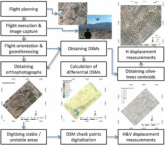
3. Materials and Methods
The methodology was based on digital photogrammetry techniques, used in previous studies by the authors [
5,
9,
16,
17], although with some variants due to the use of a UAV [
39,
40,
41] and the semi-automatic method developed to recognize common points (olive trees) between flights in order to measure displacements. The methodology can be summarized in the following steps that will be explained in
Figure 3 and the next sections:
Data capture: UAV equipment, mission planning and execution of the flights.
Georeferencing and flight orientation.
DSM, DTM and orthophotograph generation.
Comparison between observation campaigns: Measurement of displacements.
3.1. Data Capture: Unmanned Aerial Vehicle (UAV) Equipment, Mission Planning and Execution of the Flights
For this study, data from five UAV flights of very high resolution and accuracy undertaken between November 2012 and February 2016 were available. The flights were executed with two UAVs, shown in
Figure 4. The flight characteristics are shown in
Table 1 and their location and extension in
Figure 5.
The first three flights (2012, 2013 and 2014) were performed with an eight-rotor AscTec Falcon 8 [
63] (
Figure 4) coupled with GNSS/INS and equipped with a MILC (mirrorless interchangeable lens camera) Sony NEX 5N (APS-C format, 16 Mpx, pixel size 4.9 μm). The lens used was a Sony E 16 mm f/2.8 fixed focal length (24 mm in equivalent 35 mm format). The maximum takeoff weight (MTOW) was 2.3 kg and the speed was in the range of 4.5 to 15 m/s depending on the flight mode (manual, height or GPS mode). The flight times were as long as 20 min. For the fifth flight (2016), the UAV was upgraded to the new Asctec Trinity system with improved performance regarding the redundant inertial measurement unit, flight control and flight dynamic [
63].
The fourth campaign (2015) was carried out with another eight-rotor multicopter, ATyges FV-8 Drone [
64] (
Figure 4) due to the unavailability of the other UAV as it was in repair and maintenance at the time of the field survey. It is formed by a structure in carbon fiber of eight rotors, control electronics by Mikrokopter and a gyro-stabilized bench sensor holder ROLL-TILT. The ATyges FV-8 Drone is capable of autonomous flight for up to 30 min and the payload is up to 2 kg. It is equipped with a compact Canon Powershot G12 camera (CCD sensor 1/1.7, 10 Mpx, pixel size 2 μm). The lens used was a 6.1–30.5 mm f/2.8 zoom lens (28–140 mm in equivalent 35 mm format), although only the wide-angle position was set.
The flying heights were between 100 and 120 m above the terrain, which guaranteed a ground sample distance (GSD) lower than 5 cm. In any case, the flying height needed to be kept at those values since 400 feet (approximately 120 m) is the maximum height limit allowed by the Spanish regulations on the use of Remotely Piloted Aircraft Systems. Due to the moderately steep gradient of the hillslope, the strip flights were planned at different flying heights above the terrain in order to maintain a constant GSD for all the images.
The flight missions were planned with the AscTec Navigator software for the Falcon 8 and the MikroKopter-Tool free software for the ATyges FV-8 drone. The whole study area (500 m × 300 m) was covered with six strips. In the case of the Falcon 8, UAV 72 images were necessary (70% overlap and 40% sidelap), but with the ATyges system, 364 images were taken (90% overlap and 40% sidelap). The differences were given by the image acquisition mode of the ATyges system, which used a continuous shooting mode with the Canon G12 camera.
Figure 5 and
Table 1 show these flight plans.
3.2. Georeferencing and Flight Orientation
For orientation of the UAV image blocks, a GCP (ground control points) network was planned following the conventional distribution used for aerial triangulation [
18]. Blocks were oriented in the ETRS89/UTM 30N coordinate reference system (CRS). The field-surveyed GCPs were distributed all around the block periphery and additional GCP chains were measured across the flight lines [
18].
Due to the problems involved with setting up a permanent network in an unstable area, the GCPs were defined as artificial circular targets and some well-defined natural points (
Figure 6). These GCPs were surveyed with differential GNSS methods (DGNSS) in the range of centimeter accuracy with LeicaSystem 1200 and Leica Viva systems. A set of these points was not used in the orientation process but they were reserved as check points (CHKs) to validate the accuracy of this process. The number of GCP and check points are included in
Table 2.
Nevertheless, as had been tested in previous studies [
5,
16,
17,
39,
40,
41], it was possible to transfer points between different campaigns (second-order GCPs), taking one of the surveys as common reference, thereby reducing the field work in a cost-saving technique, if the points are stable, unambiguously identifiable and well distributed. This procedure involves measuring points in the reference flight and calculating their coordinates in the corresponding CRS by means of spatial intersection (PhotoScan employes a collinearity model, as other conventional photogrammetric software), and transferring them as GCPs to the other flights. The use of these points helps to improve the georeferencing of both sets of images in a common reference system, facilitating the comparison between the models and orthoimages generated from them. In this case, a sample of these points has been also used as check points. The error rates of transferred points (both GCPs and check points) are usually higher than the conventional GCPs measured by means of GNSS techniques in the field (
Table 2), although the accuracies obtained are enough for the requirements of this work, as will be discussed in the next sections.
This procedure allowed the orientation of the flight of 2013 transferring points from the flight of 2012, in addition to the flight of 2015 transferring points from the flight of 2014. Therefore, no field GNSS surveys were carried out for the flights of 2013 and 2015, in which transferred GCPs and check points were selected only in stable areas. However, it was not possible to transfer enough points to the flights of 2014 and 2016 from the previous flights as GCPs because too many of them changed or disappeared—particularly in the landslide area that dramatically modified the terrain or were difficult to identify. Consequently, GCPs were measured again in the field by means of GNSS for the flights of 2014 and 2016. For all the flights, those with GNSS-based GCPs as well as those with transferred GCPs, the points network followed a similar configuration that ensured the quality of block adjustment [
18,
26], although it did not always materialize exactly, and there were changes in the location and number of the GCPs in the different flights (
Table 2).
The images were processed and aligned by means of dense matching and Structure from Motion (SfM) techniques, which implied the automatic measurement of some 10,000–15,000 common tie points. After the measurement of the GCPs, the final photogrammetric orientations were computed using a global bundle block adjustment [
18,
25,
26]. All processes were implemented with Agisoft PhotoScan software.
The final accuracies of all adjustments are shown in
Table 2. RMS (root mean square) pixel is the reprojection error and has values usually lower than the pixel size that informs of the general quality of adjustment. The errors in the check points (CHKs), expressed also as RMS, refer to the residuals calculated in these points after the bundle adjustment. In the case of the flights of 2012, 2014 and 2016, these errors only refer to those field-surveyed (GNSS-based check points). But in the flights of 2013 and 2015, since both the GCPs and the check points were second-order points transferred from a previous flight, the errors in the transferred check points are influenced by the propagation errors (the 2012 flight on the 2013 flight and the 2014 flight on the 2015 flight). These propagation errors have been added in
Table 2. The expressions for calculating these propagation errors are:
Errors at the check points do not exceed 0.04 m in XY and 0.03 in Z in practically any case, as they are usually higher in flights with transferred points. Thus the propagation errors have values lower than 0.05 in XY and Z. Another quality control from derived products (DSMs and orthophotographs) was performed calculating the relative displacements in 151 stable points (DSM check points) distributed throughout the overall zone. The procedures are explained in the next section (DSM/DTM and orthophotograph generation) and the results are presented in the corresponding section.
3.3. Digital Surface Model (DSM), Digital Terrain Model (DTM) and Orthophotograph Generation
The Digital Surface Models (DSMs) of all flights were generated from a densification of the initial sparse point cloud (using the dense point cloud tool of PhotoScan) after the block orientation. These dense point clouds involved some 15,000,000 points as average for all flights. Then orthoimages for each campaign were also generated. Finally, both products were exported as raster files (TIFF) to be incorporated into GIS analysis.
The resolution of DSMs was 0.10 m, given that the resolution of the orthoimages was 0.05 m and the GSD even lower (0.029–0.044 m). In conventional photogrammetry the resolution of models are several times that the GSD of the images and the resolution of orthoimages generated from them. But in this case, given the new global dense matching techniques used by the current SfM photogrammetric software and taking into account the dimensions of the area and the characteristics of the flights, the pixel size of DSMs are twice the orthoimage.
Unlike previous studies [
39], in this paper the landslide evolution was monitored with DSMs instead of DTMs, because the study area presented a high density of vegetation in some sectors with grass, scrubs and bushes that had grown intensely in these last years. Under this circumstance the DTMs obtained from DSMs, using the tools of point clouds classification and filtering of PhotoScan, had only partially removed the olive trees. Stereo-model edition using photogrammetric workstations and the corresponding software was not performed because it did not ensure good results—it could not eliminate the grass and dense scrub—and would have been time consuming.
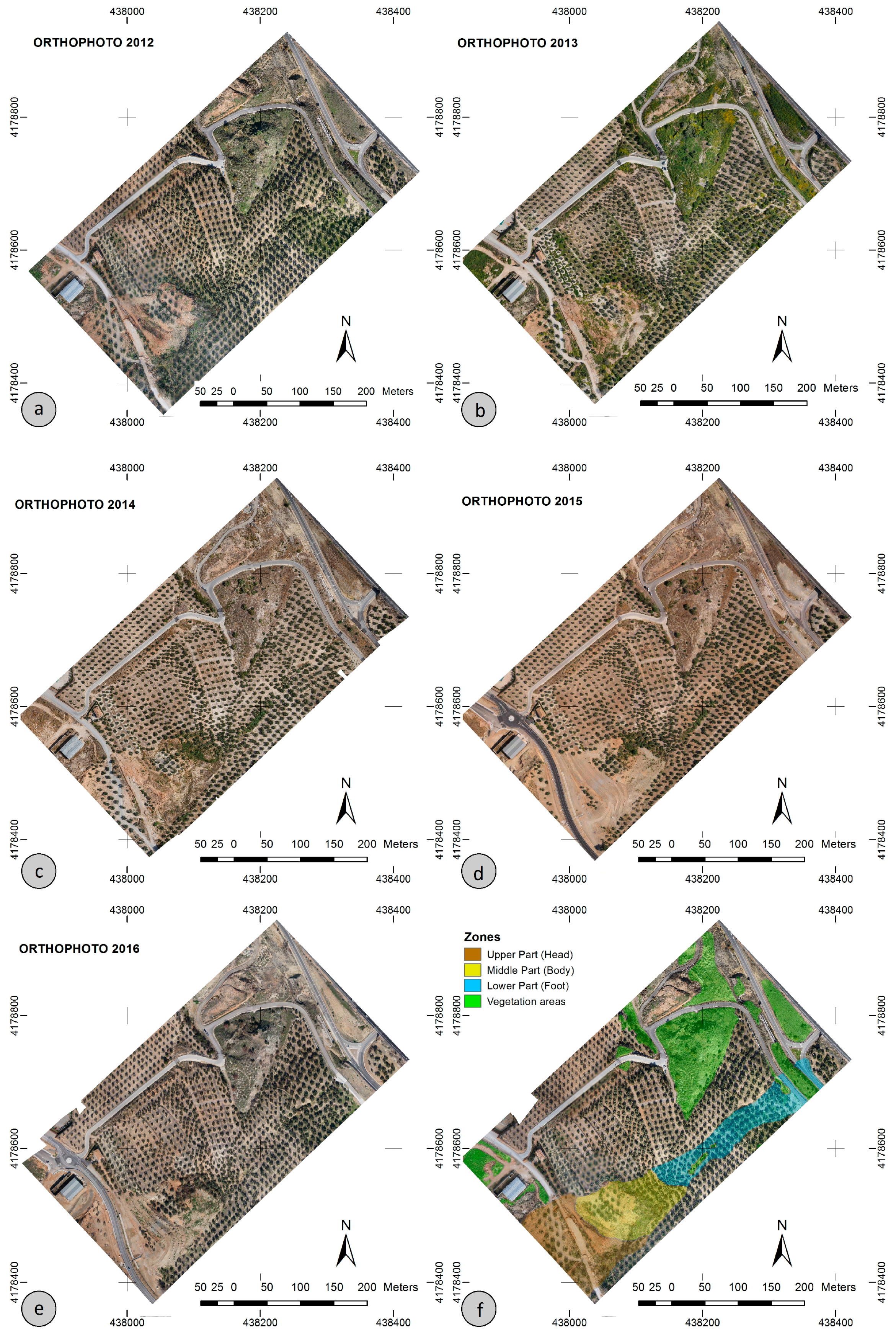
The orthophotographs, shown in
Figure 7, were obtained with a resolution of 5 cm (0.05 m), higher than GSD (0.029–0.044 m). Therefore, taking into account that the XY errors and uncertainties calculated from the flight orientation process at check points—and at the DSM check points as will be presented and discussed—are of the same order of magnitude than the resolution, the measurements made on the orthoimages can be considered as reliable.
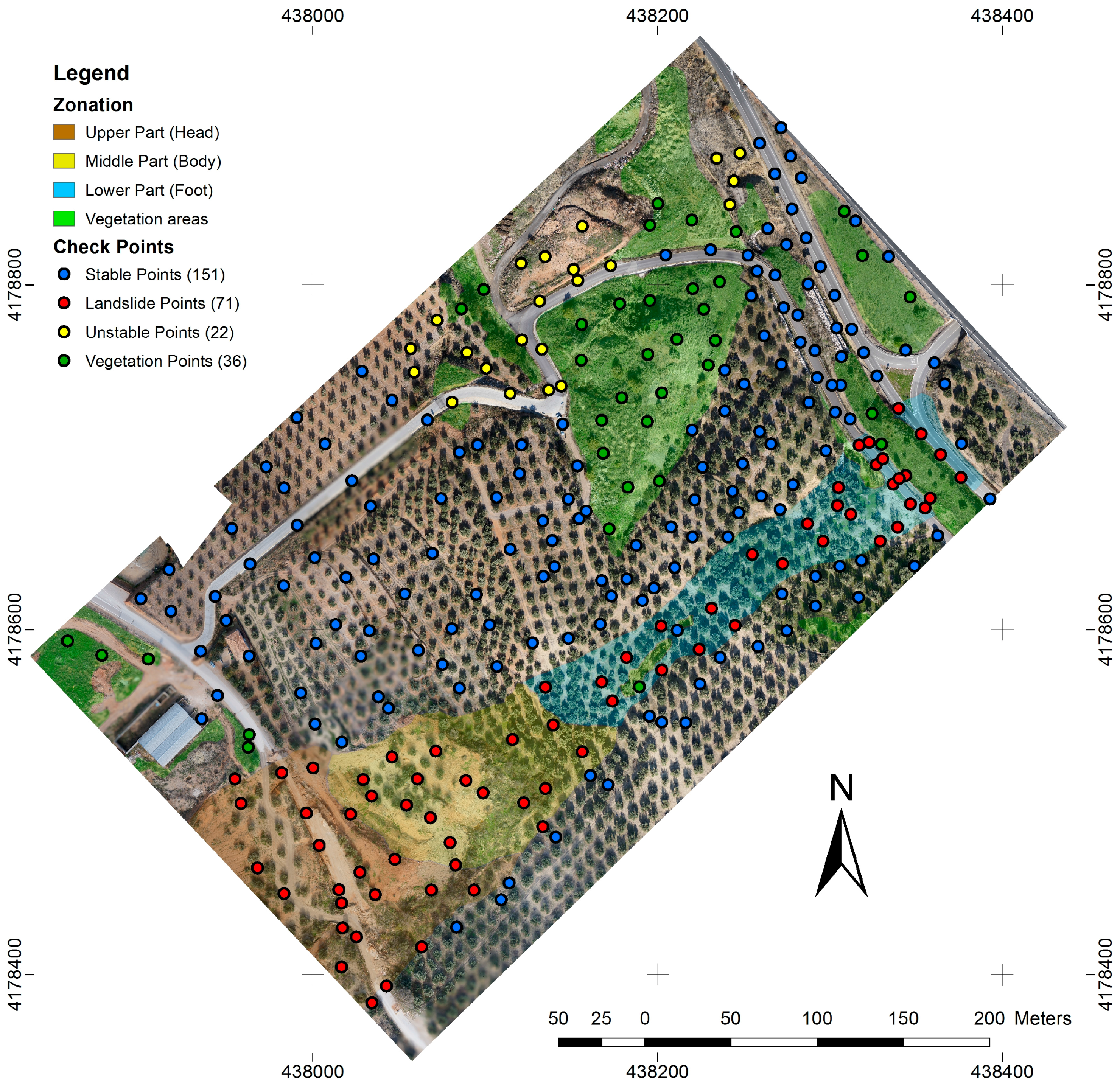
After all DSMs and orthophotographs were available, a network of 280 well-defined points visible in all orthoimages was established (
Figure 8) as DSM check points. First of all, those points located in stable areas (151) were selected as check points in order to analyze the relative adjustment between all DSMs and orthophotographs and also to validate the errors at the check points (GNSS-based and transferred) of the orientation process given in
Table 2. The results of this quality control are shown in
Table 3. Secondly, the points located in unstable areas (93), and specifically in the main landslide (71) were used to measure horizontal and vertical displacements. All these DSM check points (stable and unstable) were selected manually and placed carefully on the bare ground, which was easy because they were located in olive groves—in which the vegetation is usually removed by farming tracks and roads. Points located in areas covered by vegetation (36) have finally been excluded from the analysis.
3.4. Comparison between Observation Campaigns: Measurement of Displacements
The comparison between the different epochs has been carried out in this paper based on the products described below:
From the DSMs the vertical displacements were obtained by subtracting the pixel values between two sequential models (differential models).
From the 3D coordinates of the DSM check points extracted manually from the orthophotographs and DSMs, the vertical and horizontal displacements between points were calculated.
From the plane coordinates of the centroid of olive trees, the horizontal displacements between these features were calculated.
The comparisons between DSMs (differential models) were performed with ArcGIS and the open source software QGIS. These comparisons mainly allow the visual identification of landslide features (head and depletion area, main and secondary scarp, body, toe and accumulation area) and the estimation of vertical displacements in certain areas not covered by vegetation. But given the difficulty in obtaining a true DTM, mean values of displacements and the volumes involved were not calculated. More precise calculations of vertical and horizontal displacements were made from the coordinate measurements at DSM check points in the landslide area. These points were selected manually and located carefully on the bare ground.
Furthermore, although some techniques of automatic recognition of features based on image analysis were tested, they did not offer satisfactory results because of the dramatic changes in the orthophotographs corresponding to the different epochs. These changes were caused by different lighting conditions, deep shadows, the landslide itself, repair works and the changing vegetation cover. In some limited areas, such as roads, some results were obtained but they were considered inconclusive for this paper. In this regard, this study deals with another approach based on the automatic recognition of olive trees that cover most of the area. These elements are sufficiently distinguishable from the background to provide reliable results, but at the same time have the disadvantage of suffering changes such as growing, pruning or removal (especially in the landslide area). Being a methodological approach, the analysis was only performed between the first (2012) and the last epoch (2016), in which the displacements had a larger magnitude.
The approach uses the dense point clouds generated with PhotoScan, which are classified within the LAStools software suite. The classification process is carried out semi-automatically. The first step was the automatic classification of the dense points cloud with the Ultra Quality option in the LASground tool, using the default parameters for forest or hills areas. Then a manual edition is performed to refine the classified data. These classified point clouds are transformed into normalized clouds, which means that the points classified as terrain appear in a horizontal plane at a constant level (0) and only the points classified as non-terrain have an assigned height. Then the normalized clouds are transformed to raster images, so image processing filters can be applied in order to extract information.
The normalized raster images are segmented using a threshold value of 0.3 m. This corrects classification errors and so all elements with Z higher than 0.3 m are assigned with value 1 and the other elements take value 0. Then the centroids of the olive trees are extracted semi-automatically using GIS tools: the extracted elements are vectorized so polygons are obtained; then those polygons too small to be considered as olive trees are filtered (a threshold of 2 m2 is used); finally, the centroids of the different polygons are calculated.
This operation is performed for the point clouds corresponding to the initial (2012) and final (2016) campaigns. In order to reference the olive trees of different years and so calculate the displacements between them, it is necessary that the olive trees present the same identification in the two campaigns analyzed. This is accomplished by building buffers around the centroids, merging those buffer layers for the same olive tree in different campaigns and renaming them, thus allowing the centroids of both campaigns to be named with the same identifier.
The last phase of the process, the calculation of displacement vectors, is performed using a JAVA application developed by the authors, in which both the displacement module and direction are calculated for each of the points considered in the analysis. In total, 1100 olive trees were identified, those that remained throughout the whole period, although some of them underwent shape changes in the last campaigns.
4. Results
The results are analyzed in different sections, which essentially coincide with the different methodologies followed for comparison between campaigns: analysis of differential models, analysis of displacements at selected points and analysis of the horizontal displacements of the centroids of olive trees. At the beginning, two brief sections are presented about the results of displacements measured at stable DSM check points), and the landslide recognition and zonation.
4.1. Displacements between Models at Stable DSM Check Points
The results of displacements between models obtained at the stable DSM check points are shown in
Table 3. It can be observed that the mean errors are below ±0.02 m in XY (in the order of the GSD values) and below ±0.06 m in Z. Moreover, the RMS errors—employed in most studies [
26]—are below 0.10 m in XY and 0.13 m in Z. Finally, the standard deviation (SD) is usually less than 0.10 m in XY and Z, although in this last case some values reach 0.15 m.
4.2. Landslide Recognition and Zonation
A visual inspection and photo-interpretation of the models in the photogrammetric software, and the orthoimages (
Figure 8) and differential models (
Figure 9) in the GIS allowed the clear recognition and delineation of a landslide in the south sector. This inspection has been helped by field observations. This landslide covered the hillslope from the upper part, affecting and ruining the A-3200 road—which connects the town of Jaén with the village of La Guardia—to the lowest part in the vicinity of the A-44 highway, affecting the access way from the highway to the village of La Guardia and another road constructed to avoid traffic interruption of the A-3200 road (
Figure 2).
In the landslide mass, a head area in the upper part—very chaotic and with several scarps—and a foot area in the lower part could be clearly identified [
65]. A transitional or body area in the middle part was also distinguished. This landslide zonation is shown in
Figure 7e.
Moreover, towards the northern part of the area, a second unstable zone is identified, corresponding to an incipient landslide in which the deformation is lower and the roads only suffer cracks and bumps (
Figure 2d). The remaining areas are initially stable but these zones where there are changes in the vegetation state are also highlighted.
4.3. Differential Models
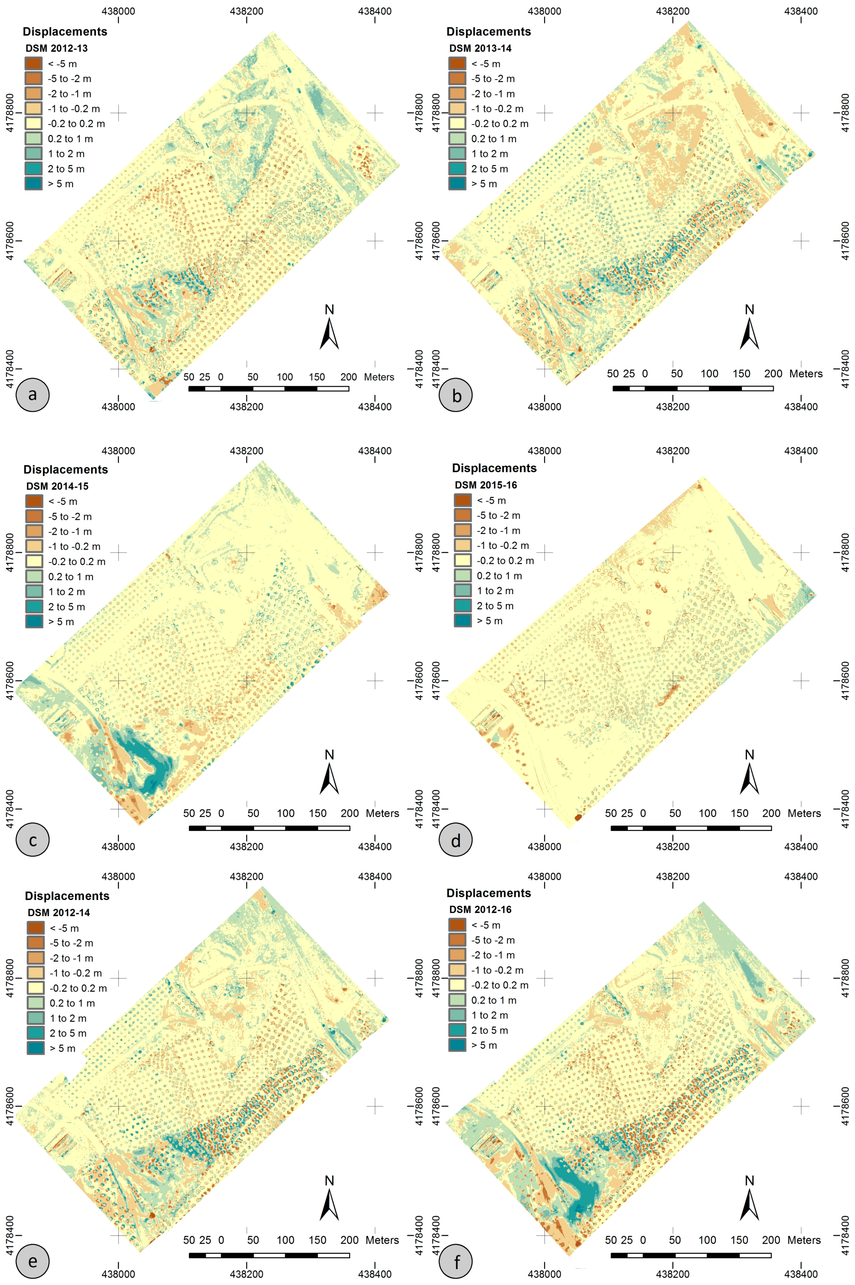
Differential models calculated from the DSMs are shown in
Figure 9. In the first two differential models (2012–2013 and 2013–2014), ignoring the effect of the zones of grass and scrub vegetation located in the central-northern sector, areas where the height of the ground surface descends and areas where the height of the ground surface ascends were observed. The first areas predominated in the upper part of the slope (zone of depletion or head) associated with the main scarp and also with secondary scarps; the latter dominated the middle and lower part of the slope, associated with the landslide foot (zone of accumulation), but also appearing at the head, alternating with depletion zones in the area where the secondary scarps were formed. Therefore, in these first periods, descents up to 0.8 m and also ascents up to 0.3 m, in alternating bands, were observed in the upper part or head zone; descents up to 0.4 m and ascents up to 1.3 m were observed in the middle part, predominating the ascents toward the lower part; finally, descents up to 0.3 m and ascents up to 0.7 m were observed in the foot area, reaching the maximum values of both cases near the access roads.
Since the 2014–2015 period, the landslide dynamic has changed dramatically at the upper and even the middle part of the hillslope, where large vertical displacements of the terrain surface were observed, both in terms of depletion and uplift zones. In the lower part of the landslide, the situation is completely different, and only smooth terrain ascents were observed. Thus, in the period of 2014–2015, we were able to observe descents of up to 1.2 m and ascents up to 1.5 m in the upper part, above and below the new road A-3200; descents up to 1.0 m and ascents up to 1.2 m in the middle part, with the maximum absolute values in this case towards the upper part; and descents up to 0.15 m and ascents up to 0.2 m in the lower part, with the maximum values also in the zone near the access roads. Finally, in the last period studied (2015–2016), scarcely any changes occurred on the surface of the ground in the landslide area and its surroundings.
4.4. Analysis of Displacements at Unstable DSM Check Points
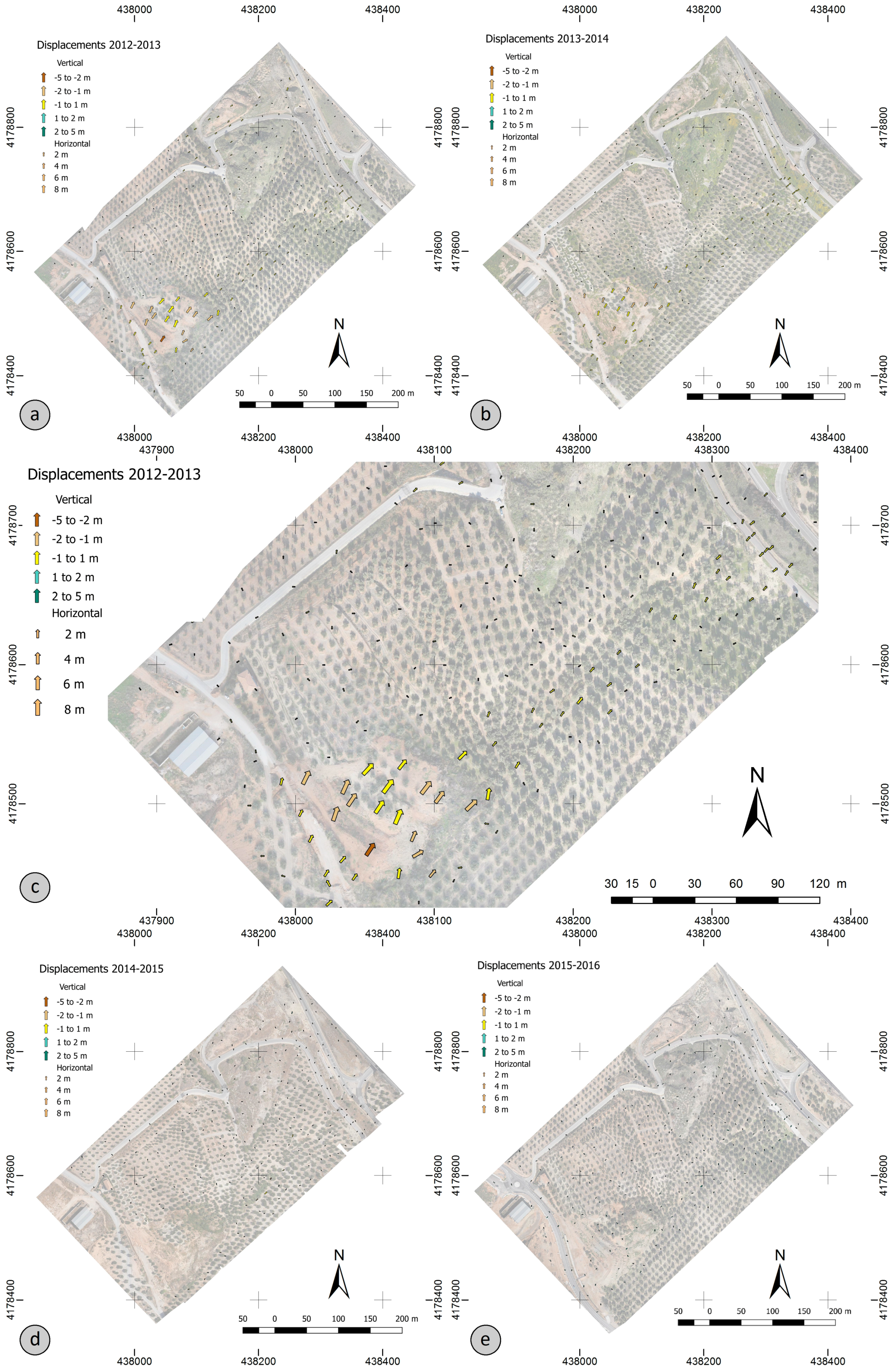
This analysis is shown graphically in a map of displacement vectors in the
Figure 10 and it is summarized in
Table 4 for the different parts of the main landslide area. The mobilized and stable areas can be clearly distinguished on the map of displacement vectors.
In this case, the largest displacements towards the northeast are located in the main landslide area, while the remaining zone presents much smaller displacements without a clear direction. Also, in the northern sector, an incipient unstable zone is observed, although the displacements are not so large.
Table 4 shows the mean values (absolute and rates) of the displacement vector modules in the vertical and horizontal component, as well as the mean direction and the mean length of the resultant vector (MLRV). MLRV is a measure of circular dispersion, the directions being more uniform when it is close to 1 and more dispersed when it is far from 1 [
66]. The horizontal displacements observed in
Table 4 are an order of magnitude higher than those in the vertical displacements. From the absolute values of displacements, the rates of displacements are calculated, dividing the absolute values by the period of time between campaigns (expressed in years).
The vertical displacements measured at landslide DSM check points were usually negative, so the points tend to descend as the movement progresses. Thus the descent rates in the first period reached 1.428 m/year in the upper part of the hillslope, 1.920 m/year in the middle part and 0.129 m/year at the lower and less steep part. These descent rates were of 0.338 m/year, 0.732 m/year and 0.160 m/year at the upper, middle and lower parts respectively, in the second period. In the third period (2014–2015), most points in the upper and middle part disappeared, while in the lower part, the vertical displacements of the points were not significant. The same happened in the fourth period (2015–2016) in this case for all the sectors of the landslide.
The analysis of horizontal displacements shows that in the first period considered (2012–2013), large displacement rates higher than 4 m/year and 13 m/year m occurred, respectively, in the upper and middle areas, while in the lower part, the rate was about 1.4 m/year. In the second period (2013–2014), horizontal displacement rates decreased to 1.146 m/year in the upper part, 3.304 m/year in the middle part and 0.778 m/year in the lower part. In the third period (2014–2015), the points in the upper and middle part disappeared again, whereas in the lower part, horizontal displacements with rates of about 0.268 m/year remained. Finally, in the period 2015–2016, the horizontal displacements were practically null or not significant in all parts of the hillslope.
The mean direction of displacement vectors is northeast (NE). This direction remained practically constant (between 048° and 057°) throughout the first (2012–2013) and second period (2013–2014). The mean length of the resultant vector presented values close to 1 in the first and second periods, although in the upper part, values of around 0.8 were observed. These parameters decreased to below 0.5 in the third (2014–2015) and fourth periods (2015–2016).
4.5. Analysis of the Horizontal Displacements of the Olive Tree Centroids
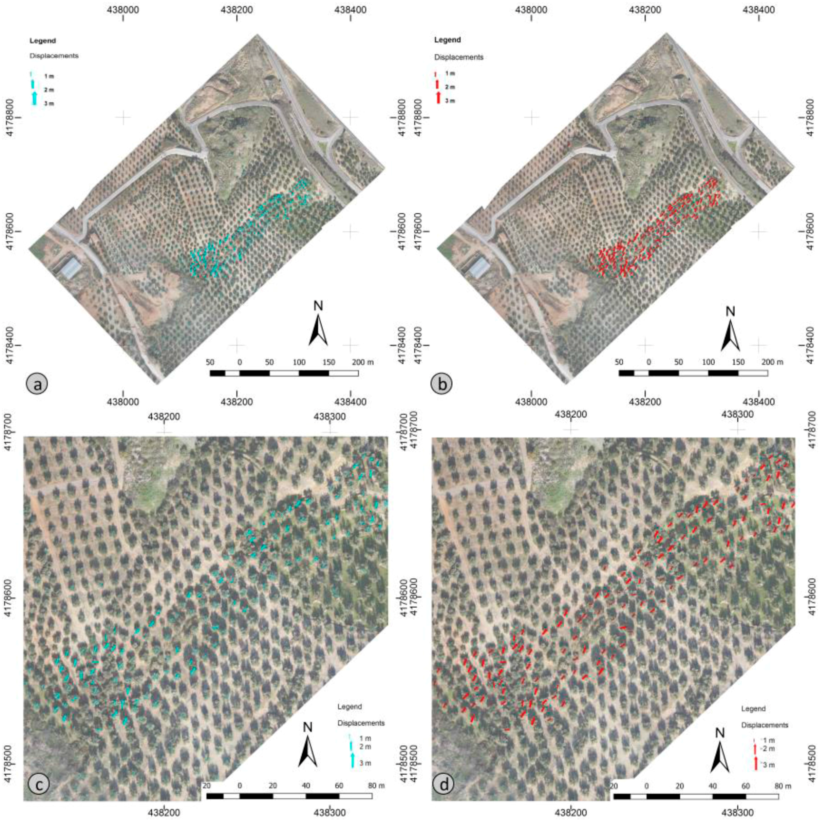
This analysis, based on a semi-automatic approach, also allows a mapping of the deformation, although restricted only to the horizontal component of displacement.
Figure 11 shows a map of deformation based on this approach where the mobilized area is clearly differentiated from the surrounding stable area. The mean displacement modules and directions of the period 2012–2016 are shown in
Table 5. The larger horizontal displacements were observed in the middle part (2.832 m), followed by the lower part (2.452 m) and the upper part (1.336 m), and the shorter values were in the stable area (0.719 m). The mean direction was towards NE in the different parts of the landslide and towards the SSW in the stable area. Finally, the MLRV was at its maximum in the lower part (0.907 m), the middle part (0.815 m) and the upper part (0.716 m) and minimum in the stable area (0.176 m).
However, since olive trees are irregular features that can change their physical appearance because of pruning, growth, etc., different types of filters were tested in order to identify displacements due only to landsliding. Firstly, several local statistics of the displacement vectors (mean module, mean direction and mean length of resultant vector) were calculated in a buffer of 15 m around each centroid. It can be noticed that in mobilized areas the vector modules have clearly higher values than in stable areas. In fact, in stable areas, the displacements due to changes in the shape of the olive treetops are less than 1 m, while in landslide, the displacement values are usually up to 2 m and higher. Moreover, in the mobilized areas, the vectors have a more uniform direction (NE) and the mean length of the resultant vector has higher values (close to 1) than in stable areas.
The module and direction of the displacement vectors were therefore selected as filters and, subsequently, those vectors with modules lower than 1 m were eliminated. Moreover, those vectors with a direction value of ±60° with respect to the mean direction of the landslide displacement (rounded to 050°), which means directions between −10° (350°) and 110°, were also eliminated. The result of the application of these filters is also shown in
Figure 11.
5. Discussion
The discussion deals with different aspects of the previous sections. Firstly, some considerations about the limits of accuracy of the study will be presented, based on the results of the orientation and georeferencing process and the analysis of check points. Secondly, the results of the analysis of differential models, analysis of displacements at selected DSM check points and analysis of the horizontal displacements of the olive tree centroids will be discussed. Then a brief description of qualitative aspects extracted from these analyses will be given. The section will finish with some conclusions regarding the relationships between the trigger mechanism of the landslide (rainfalls) and its kinematics.
5.1. Accuracies, Errors and Uncertainties
The RMS errors referring to the GNSS-based and transferred check points after the bundle adjustment do not exceed 0.04 m in XY and 0.03 m in Z in practically any case (
Table 2), neither in the flights oriented by GNSS-based GCPs (2012, 2014 and 2016) nor the flights oriented by second-order points (2013 and 2015) transferred from a previous flight (2012 and 2014, respectively). In the last cases, the propagation errors are also taken into account showing values lower than 0.05 m. These errors are of the same order of magnitude than the image resolution, as it has been described in previous comparable studies [
26,
32,
34,
38,
42,
44,
45] with similar properties (equipment, flight altitude and resolution).
From the displacements measured between the 151 DSM check points placed on the bare ground in stable zones, the mean errors, RMS errors and standard deviation (SD) were calculated (
Table 3). RMS errors also show values of the same order of magnitude of those calculated in this work at GNSS-based and transferred check points, and those found in the aforementioned studies with similar properties. In these studies, the RMS calculated in GNSS-based check points are in the range of 0.05–0.10 m [
32,
38,
45] or even higher [
34]. In a lower resolution study [
31], a value of 0.50 m is found in the comparison of UAV and LiDAR DSMs, where DSM check points are used in the same way as in this study. Other studies, also of lower resolution, in which the errors in ortophotographs and DSMs are around 2–3 times the resolution of images, agree with these observations [
28,
29].
Furthermore, it can be observed that the mean errors at the DSM check points are below ±0.02 m in XY (in the order of the GSD value) and below ±0.06 m in Z, which confirms the good general adjustment or centering of the models, without systematic horizontal or vertical displacements; however, there can be local misalignments as the higher values of RMS and SD reveal. In this way, the standard deviation, which is actually a measure of the uncertainty of the data, is usually lower than ±0.10 m in XY and Z, although in this last case, some values reach ±0.15 m. It can be established that the general adjustment models between flights are very fine (better than 0.06 m in XY and Z), while the uncertainty, and so the accuracy, is 0.10 cm in XY and 0.15 cm in Z. Thus higher displacement values with respect to these thresholds allow us to deduce changes in the ground surface, while lower values are inconclusive.
5.2. Differential Models
Differential models (from DTMS or DSMs) are calculated in many studies in order to study the landslide evolution [
30,
31,
34,
35,
36,
39,
40,
41,
45]. In this study, DTMs are obtained by classifying and filtering DSMs, but only olive trees could be partially eliminated, while the grass and scrubs remained. In these conditions, DTMs and the differential DTMs do not improve significantly in respect to DSM and differential DSMs. Therefore, the use of differential DTMs does not allow more precise evaluations of displacements and volumes. Thus differential DSMs are used in this work to make visual observations of the landslide features and evolution and to calculate approximate and local vertical displacements by means the GIS tools in some areas not covered by vegetation.
Differential DSMs between 2012 and 2014 allowed the clear delineation of the main landslide, with notable changes in the terrain surface, regarding the stable zone in which these changes were not significant. Moreover, the depletion area in the upper part (head) of the landslide, where descents of the terrain surface predominated, could be distinguished from the accumulation area in the middle (body) or lower part (foot), where ascents of the terrain surface predominated. In reality, the ascent of terrain surface in these zones was not due to an uplift of the terrain surface but to an advance of the landslide mass in the accumulation area (body and toe). This type of evolution has been observed in other studies [
6,
7,
8,
10,
11,
12,
13,
14,
15,
31,
34,
35,
36,
37,
38,
39,
40,
41,
45] with different types of landslides and it is related to displacements of the terrain surface in both the vertical and in the horizontal direction.
The absolute values of vertical displacements were similar in the upper and middle part where the maximum deformation concentrated. In the head, the alternating bands of terrain descents and ascents were due to the formation of secondary scarps and the mass advance. This area also presented higher slope-angles, alternating between very steep scarps and flatter zones, although always inclined downslope without rotational evidences. In the middle part or landslide body, the maximum ascents of terrain surface could be observed, evidencing an accumulation zone where the landslide foot began. This zone also presented higher slope-angles, as corresponds to the upper part of the foot. In this point, there is a narrowing of the landslide shape due to the original relief—in part modeled by older landslides—with zones of higher slope-angles at the flanks and a lower inclined area between them throughout which the landslide was able to advance. Nevertheless, this morphology could have stopped the landslide partially, giving rise to the formation of this steep foot at the middle of the hillslope, although the movement continued downslope. So, in the lower part, the foot had lower slope-angles and could open moderately after the narrowing. The observed ascents of the terrain surface were lower, as corresponds to a smooth foot where there is a greater horizontal than vertical development. In fact, in this zone, the vertical displacements were of the order of Z uncertainty, but in some sectors—such as the affected roads—an advance of the mass and a certain uplift of these features, due to the push on a rigid structure, could be clearly observed.
The landslide kinematics changed along the full time period studied. The largest vertical displacement rates thus occurred during the first period (2012–2013), slowing in the second period (2013–2014), though retaining the same pattern. In the third period (2014–2015), the evolution of the upper part of the hillslope underwent great changes as the result of the repair works for stabilization and construction of the new road JA-3200, while in the middle and lower part, a residual movement still remained, although the values in the order of uncertainty are not conclusive. In the last period (2015–2016), the landslide finally stopped and significant changes in the ground surface could not be observed.
Very interesting are the effects of the displacements of olive trees observed in the differential DSMs because of the landslide movement. Thus, in certain areas, some strips with surface uplifts and descents are observed. The vertical displacements range between 2 and 3 m (approximately the height of the olive trees) and they do not correspond to vertical movements but rather horizontal displacements of the tree lines.
5.3. Analysis of Displacement at Unstable DSM Check Points
The displacement vectors both in the vertical and the horizontal components allowed us to distinguish between mobilized and stable zones, as has been described in previous studies [
6,
8,
15,
34,
35,
39,
40,
41]. In general terms, the largest vector modules and the maintenance of uniform directions are indicative of those zones where movements occur.
In the study area, two unstable zones were identified, one corresponding to a more developed landslide in the southern part, with larger displacements, and the other one in the northern part, in an incipient state with shorter displacements.
Focusing on the main landslide, it could be observed that the horizontal displacements were an order of magnitude higher than the vertical displacements, which is consistent with the kinematics of a flow type movement where the horizontal component is greater than the vertical [
55,
56,
67,
68]. Moreover, the usually negative values of vertical displacements show that the points tend to descend as the landslide progress, unlike what happened in differential models where the observed uplifts are due to the mass advance and accumulation.
As in the analysis of differential models, two different stages could be observed before and after the stabilization works. The maximum descent rates were reached in the first period (2012–2013), being larger in the upper (head) and middle part (body) than in the lower part (foot), where the horizontal component of the movement predominated, according to a typical flow-type movement with formation of scarps in the head. According to the average data, the vertical displacement rates of DSM points slowed in the second period (2013–2014), except in the foot, which indicates transmission of the movement downslope, after the movement in the head and body was stopped by the narrowing and also by the rainfall decrease. In both periods, the absolute values of vertical displacements were significantly higher than those values found in the stable zones (
Table 3), where mean values did not exceed 0.06 m and the RMS and SD were lower than 0.10–0.15 m. In both periods, the movement can be catalogued as slow, according to the suggested classification of WP/WLI [
69] and the available data (one campaign per year), although it is possible that it reached moderate velocities in some rainy event, like in some movements analyzed in surrounding zones [
39,
40,
41].
In the third period (2014–2015), the disappearance of points in the upper and middle part was due to the repair works (the landscape changed completely). Meanwhile, in the lower part, the vertical displacements of the points were not significant, as the absolute values were below the accuracy limit (0.15 m) estimated from the standard deviation of stable points. The same occurred in the fourth period (2015–2016) for the whole landslide, as a consequence of stabilization works.
Similar considerations could be established from the analysis of horizontal displacements. The largest displacement rates of several meters per year were reached in the first period (2012–2013) in the upper (head) and middle (body) part, where the larger deformations occur, and shorter (about 1.5 m/year) in the lower part (foot). The velocity was from slow to even moderate (in the upper parts). Again, the more active zones were the head, the body and even the starting point of the foot, where the slope-angles were higher, while in the lower part of the foot—after the narrowing—the slope angles were lower and the movement more residual. The rates slowed in the second period (2013–2014) to values close to 1 m/year (slow velocity). In any case, in both periods, the mean absolute horizontal displacements were much larger than those calculated in stable areas (0.02 m), the orthoimages resolution (0.05 m) and the accuracy limit (0.10 m). In the third period (2014–2015), ignoring the points that disappeared in the upper and middle part, residual displacement rates in the lower part could be observed. As in the previous analyses, the horizontal movements were practically null in all parts of the hillslope in the fourth period.
An average direction of the horizontal displacement towards downslope (NE), and high values of the mean length of resultant vector—low dispersion of directions—were found in the landslide area in the first periods (2012–2014). This low dispersion of the directions of displacement vector suggests a fairly coherent movement, despite being a flow in which the movements tend to have a chaotic behavior [
55,
56,
67]. It confirms the earth-flow typology in which the movement is more coherent than other flow types, including mud flows or debris flows. Nevertheless, the higher dispersion observed at the head suggests a more chaotic pattern in this area of greater deformation.
On the contrary, directions different to the general trend of the hillslope and lower values of the mean length resultant vector—high dispersion of the directions—appeared in stable areas. In these areas, the displacement should really be null and without a set direction. So the short modules and the high dispersion in the directions found in these stable areas seems due to the limit of precision in the positioning of measurement points and not to a real displacement of the terrain. The same can be said about the landslide area when the movement stopped (since 2014).
5.4. Analysis of the Horizontal Displacements of the Olive Tree Centroids
This analysis, based on a semi-automatic approach that allows a mapping of the horizontal deformation and identification of potential unstable areas, is original of this study. However, the methodology has its limitations because the elements selected to evaluate the displacements—the olive trees—are irregular features that can change their physical appearance because of pruning, growth, etc. Some approaches based on techniques of expertise classification of point clouds to detect objects such as trees and their parts (trunks, branches, etc.) [
70] or taking into account properties of DSMs (heights, slopes …) and the orthoimages (radiometric bands) could refine the methodology. In this work, however, we have followed a simple approach based on applying filters in order to distinguish true displacements due only to landsliding from other possible changes.
The mean displacement modules and directions calculated for the whole period (
Table 5) show differences between stable areas and the different parts of the landslide. The maximum horizontal displacements are observed in the middle part followed by the lower and the upper part, coinciding roughly with the analysis of the DSM check points. However, the displacements between olive centroids are not as large as between check points, especially in the upper and middle parts, because the olives in these areas of maximum deformation have disappeared (in fact, in the upper part, there are only six olives and the measurements are not significant). In stable areas, the displacements are shorter than in the landslide areas, but higher than those observed in the DSM check points, due probably to the irregular shape of olive trees and the low accuracy in the centroid position. It agrees with the mean values of directions of displacement and MLRV; the directions in the landslide area are quite uniform (high values of MLRV) and, towards NE (downslope), they coincide with the values observed in the DSM check points. However, the stable areas are very irregular (low values of MLRV) and even upslope. In these cases, the irregularity is larger than in the DSM check points, due to less accuracy in the positioning of olive tree centroids.
Thus, in order to distinguish the unstable areas from the stable ones, different filters were tested based on local statistics of the displacement vectors (mean module, mean direction and mean length of resultant vector) calculated in a buffer of 15 m around each olive centroid. The mean module and direction of the displacement filters operate efficiently and so those vectors with a module lower than 1 m and with a direction value of ±60° with respect to the mean direction of the landslide displacement were eliminated. The remaining vectors highlight the main landslide area in the south part and also the incipient unstable area in the north.
With respect to the other statistical parameter, the mean length of the resultant vector also shows the mobilized areas clearly, but this coefficient presents some problems since its distribution is highly irregular near the boundary between stable and unstable areas. Moreover, in areas affected by flow type landslides with a chaotic behavior, the use as filter of the mean length of the resultant vector could lead to error.
It can be thus concluded that the application of these filters results in the delimitation of the movement (
Figure 11), thereby validating this semi-automatic recognition method that can be applied to the detection of movements in areas of olive groves or other groves that follow a regular pattern.
5.5. Qualitative Characterization of the Landslide
A visual inspection in the field as well as the previous analyses show a slope movement of earth-flow type [
55,
56,
67]. This type of slope movement is defined as “rapid or slower, intermittent flow-like movement of plastic, clayey soil, facilitated by a combination of sliding along multiple discrete shear surfaces, and internal shear strains (with) long periods of relative dormancy alternating with more rapid surges” [
56]. The velocity (catalogued in this case as slow to moderate), the plastic marls and clays of the Guadalquivir Units [
54,
58,
59,
60,
61,
62] outcropping in the study area and the slope-angles (ranging from 5° to 20°) are characteristic of this landslide typology. Additionally, the water sources from the carbonate materials of the surrounding reliefs—and also by the colluvial deposits—during the rainy periods contributed to the landslide origin and evolution.
The landslide presented a crown area [
65] in the upper part located in the surrounding area of the road JA-3200. This road, which connects the village of La Guardia and the city of Jaén, was affected by the landslide and had to be repaired (
Figure 2). The shape of this crown was rounded and the head inside had several successive moderate scarps up and down the road, ending in a back-scarp at the road cut. Among the scarps some flat areas appeared as relics of the original relief. These areas were not inclined counter-slope, but moderately downslope, so there was no evidence of rotational mechanisms. As the landslide progressed, the tension cracks grew upslope and eventually affected the constructions of the top of the hillslope (an olive oil mill and roads). All these features were formed mainly in the colluvial or piedmont deposits coming from the surrounding reliefs that cover a high proportion of the area. These materials are more coherent and facilitate the formation of scarps and tension cracks.
The landslide mass had a rather disorganized sector in the head or upper part of the landslide (
Figure 7,
Figure 8,
Figure 9,
Figure 10 and
Figure 11), where the largest deformation occurred between 2012 and 2014. This upper area—now dismantled after the repair works—was in general a depleted zone and contained abundant transverse cracks. It also had a well-defined lateral boundary and ended in an accumulation zone that extended throughout the body and the foot of the landslide. This accumulation zone formed a shoulder in the terrain surface characteristic of a foot zone, but the movement did not finish at this point and continued downslope after a narrowing in this middle area (
Figure 7), that can be still observed in 2016, although with a much smaller deformation. This narrowing in the middle part of the landslide as a consequence of the original terrain surface could stop or slow the movement and produce the shoulder. After the narrowing, the mass ran along a gentle slope to the tip of the landslide located near highway A-44, seriously affecting the access road to La Guardia from the A-44 highway (
Figure 2). In the lower part, the lateral limits were more moderate and only appeared as a crack.
The estimated mass thickness is quite small, probably no more than 10 m. Taking into account the length, about 500 m, and the depth-length ratio, about 1%–2%, the landslide belongs to a flow type movement [
68].
As well as the main landslide, some other unstable areas can be observed in the northern part of the study area (
Figure 7,
Figure 8,
Figure 9,
Figure 10 and
Figure 11). In most cases, only the development of cracks and steps occurred. These affected the temporary road constructed in order to avoid the traffic disruption of the JA-3200 road (
Figure 2d). At the bottom of the slope a differentiated movement in an incipient state with a well-formed scarp appeared.
5.6. Relationship between Rainfall and Landslide Activity
The previous analyses agree that between November 2012 (first UAV flight) and July 2014 (third UAV flight) a slope movement of flow type remained active on a hillslope near the village of La Guardia, which affected the JA-3200 road connecting this village with the city of Jaen. From July 2014 to February 2016, a stabilization of the movement was observed and the landslide only maintained some residual movements in localized areas.
Rainfall has been considered one of the main triggering factors of landslides [
71,
72] all over the world but also in the Mediterranean countries [
73], as has been demonstrated in regions close to the study area [
74].
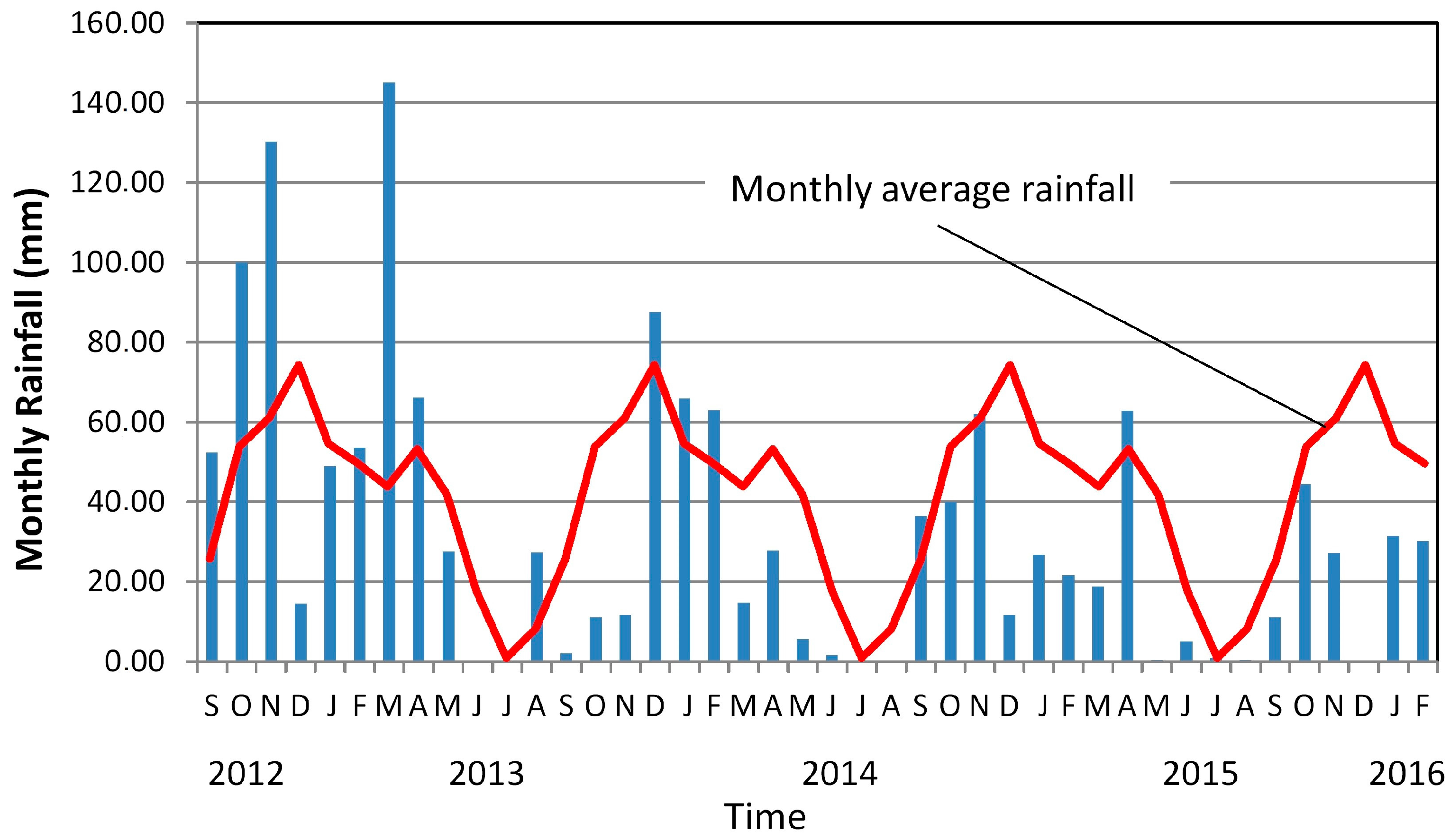
Figure 12 shows the monthly rainfall measured for this period and also the monthly average. The monthly average presents an absolute maximum in autumn and winter months (October to January) and also a relative maximum in spring (April), while the minimum values occur in summer. Moreover, the monthly rainfall shows an irregular distribution typical of the Mediterranean climate of southern Spain where cycles alternating between dry and wet years occur [
75,
76]. At the beginning of the period, between 2012 and 2013, the rainfall values were significantly higher than the average, whereas at the end of the period, especially between 2015 and 2016, the rainfall decreased below the average.
More precisely, between the flights of November 2012 and April 2013, the landslide was very active and this activity coincided closely with two periods of heavy rains where values close to 200% of the average rainfall in the area were reached. The first period occurred between September and November 2012 and the second one between February and April 2013, as described in previous studies of neighboring areas [
39,
40,
41]. The landslide activity was maintained—although reduced—for the next period between April 2013 and July 2014, perhaps discontinuously as described in the aforementioned studies. Therefore, after April 2013, a drier period began, only interrupted in August by an extraordinary peak near 300% of the average value, and between December 2013 and February 2014 in which 120% of the average value was reached.
After these periods of more intense activity, the movement had little activity, coinciding with the works of stabilization and restoration of the hillslope and the road and, at the same time, with a fairly dry period with values below 50% of the average rainfall except for a few months where the rainfall occasionally exceeded 100%. This intermittent character is typical of the earth flows in Mediterranean or arid climates [
56]. In this sense, the landslide that can be catalogued as slow to moderate following velocity classifications is also characterized as type VII of the diachroneity classification (landslides active in a period between one and ten years) [
4].
In conclusion, a certain relationship between activity and rainfall is observed, although the execution of works of stabilization of the slope interrupted the analysis and prevented more definitive conclusions from being reached.
6. Conclusions
The use of Unmanned Aerial Vehicles (UAV) is a useful tool for fast, very high resolution and precise surveys in areas of about 0.01 to 100 km2. This paper proposes a methodology for the analysis of slope instability processes. In this sense, light equipment, such as that used in this study, is well suited for updates and landslide monitoring, and thus for disaster management. It allows working with intermediate scales between terrestrial techniques (global navigation satellite system (GNSS), classic surveying, terrestrial laser scanner, terrestrial photogrammetry, etc.) and aerial or space surveys (conventional aerial photogrammetry and light detection and ranging (LiDAR), very high resolution satellite remote sensing, Differential Synthetic Aperture Radar Interferometry (DInSAR)). At this scale, detailed morphological features can still be observed, while allowing relatively large areas to be covered. Light UAVs are very agile and easy to operate compared to other heavier equipment. Also, field surveys can be performed within a few hours of work, including the measurement of ground control points (GCPs).
Since these light UAVs can also be equipped with different sensors (infrared cameras, LiDAR, Radar, etc.), their potential will increase. The use of conventional photogrammetric and Structure from Motion (SfM) techniques [
26] allows us to orient UAV flights and to obtain Digital Surface Models (DSMs)/Digital Terrain Models (DTMs) and orthophotographs from which vertical and horizontal displacements and volumetric changes can be calculated. As it has been presented in the introduction section, some studies have made advances in co-registration methodologies of multi-temporal image datasets by means of points or surfaces, the development of algorithms for detecting surface motions, and the implementation of methods of direct orientation from in-flight parameters. However, the elimination or reduction of GCP (a time-consuming task) is not yet possible in all circumstances unless more accurate positioning and inertial systems can be used on board light UAVs, although these new systems will soon be available.
In this study, both DSMs and orthophotographs at different epochs have been obtained from aerial photographs of the UAV surveys, using a methodology based on conventional photogrammetry and SfM techniques. The results obtained have allowed the characterization of the slope movement flow rate and some morphological features (crown, scarps, head, lateral limits, tension cracks, foot, etc.) on a hillslope of hectometric dimensions. In this way, the movement has been classified as an earth flow, based on the observations made on the field, the DSMs and the orthophotographs. The technique also allows a monitoring analysis by calculating differential DSMs in order to measure vertical displacements and identify depletion and accumulation areas inside the landslide. At the same time, the measurement of displacements between points selected in a manual way from the orthophotographs and models (DSM check points) allows us to analyze landslide kinematics and activity with an accuracy of about 10 cm in XY and 15 cm in Z. This accuracy has been established by means of an analysis of displacements measured in the GIS between the DSMs at 151 check points placed on the bare ground in stable zones. The uncertainties correspond to the standard deviation of these measured displacements at stable points.
In this sense, the observed displacements in the main landslide area reached values from decimeters to meters in the vertical component and several meters in the horizontal component, significantly larger than the accuracy limit. As the periods between UAV campaigns are more or less one year, the displacement rates ranged from decimeters to meters by year in the vertical direction and from 1 m/year to 10 m/year in the horizontal direction, so the landslide can be catalogued as slow (to moderate). Nevertheless, the displacement rates varied along the whole studied period and depended on the part of the landslide. Therefore, the maximum rate was reached at the beginning (2012–2013), but the landslide was gradually slowing until it stopped completely by 2015. Moreover, the areas with larger deformation were the upper part (head) and the middle part (body and the starting of the foot) of the landslide, while the area less deformed was the lower part (the smooth foot downslope).
The displacements have been correlated to the rain events that occurred in the region between the different epochs. These first analyses show a higher activity of the landslide—larger vertical and horizontal displacements—in the rainy periods at the beginning of the study, then a residual activity and finally a stop of the landslide in the following dry period, coinciding with the stabilization works of the landslide slope.
Automatic techniques of feature recognition, proposed in some studies, have been tested in this study, but they have not worked because of the changes in solar illumination, deep shadows, seasonal and inter-annual vegetation, the landslide itself and the repair works that have occurred in this zone. Nevertheless, an approach based on olive tree recognition by means of DSM classification and filtering has been applied in a groundbreaking way. The horizontal displacement measured between olive tree centroids coincide roughly with those observed between DSM check points but the disappearance of many trees in the areas of maximum deformation (the upper and middle zones) and the lower accuracy in the positioning of the centroids make the difference between stable and landslide areas less clear than in the analysis of DSM check points. In this way, the application of filters using displacement modules and directions allows a better differentiation between stable and unstable areas and thus the recognition of landslide areas. This methodology can be employed in the study of landslide activity in olive groves and other similar areas.
Future work will deal with advances in the methodology, regarding the reduction of ground control points and applying methods of direct orientation and other techniques of automatic detection of surface motions based on expert classification techniques from DSMs and images even in complex areas. Other sensors can be incorporated both in the spectral domain (i.e., near and thermal infrared sensors) and in the geometric domain (LiDAR and RADAR). Even terrestrial probes (rain, humidity, movement) in wireless networks (WSN) can be used. Other areas of interest will include the mapping and analysis of morphological features, such as cracks, scarps, steps and landslide limits.


 ,
, 


