Mapping Smallholder Wheat Yields and Sowing Dates Using Micro-Satellite Data

Abstract

Remote sensing offers a low-cost method for developing spatially continuous crop production statistics across large areas and through time. Nevertheless, it has been difficult to characterize the production of individual smallholder farms, given that the land-holding size in most areas of South Asia (<2 ha) is smaller than the spatial resolution of most freely available satellite imagery, like Landsat and MODIS. In addition, existing methods to map yield require field-level data to develop and parameterize predictive algorithms that translate satellite vegetation indices to yield, yet these data are costly or difficult to obtain in many smallholder systems. To overcome these challenges, this study explores two issues. First, we employ new high spatial (2 m) and temporal (bi-weekly) resolution micro-satellite SkySat data to map sowing dates and yields of smallholder wheat fields in Bihar, India in the 2014–2015 and 2015–2016 growing seasons. Second, we compare how well we predict sowing date and yield when using ground data, like crop cuts and self-reports, versus using crop models, which require no on-the-ground data, to develop and parameterize prediction models. Overall, sow dates were predicted well (R² = 0.41 in 2014–2015 and R² = 0.62 in 2015–2016), particularly when using models that were parameterized using self-report sow dates collected close to the time of planting and when using imagery that spanned the entire growing season. We were also able to map yields fairly well (R² = 0.27 in 2014–2015 and R² = 0.33 in 2015–2016), with crop cut parameterized models resulting in the highest accuracies. While less accurate, we were able to capture the large range in sow dates and yields across farms when using models parameterized with crop model data and these estimates were able to detect known relationships between management factors (e.g., sow date, fertilizer, and irrigation) and yield. While these results are specific to our study site in India, it is likely that the methods employed and the lessons learned are applicable to smallholder systems more generally across the globe. This is of particular interest given that similar high spatio-temporal resolution micro-satellite data will become increasingly available in the coming years.

1. Background and Rationale

Food security will become increasingly challenged over the upcoming decades by climate change [1,2], natural resource degradation [3], and a burgeoning global population [4]. Smallholder farming systems are of particular concern given that farmers often do not have access to the inputs and technologies necessary for high-production agriculture [5], and many of these systems are distributed across the tropics, where negative climate change impacts are expected to be greatest [2,6]. One way to enhance food security is to examine production levels, and identify factors associated with existing yield gaps. Remote sensing offers a low-cost way to obtain crop production statistics across large spatial and temporal scales [7,8]. However, to date it has been difficult to map the production of smallholder farms, given that the size of an individual field (<2 ha) is typically smaller than the spatial resolution of most freely-available satellite imagery (e.g., 30 m Landsat, 250 m MODIS; [9,10]). While these satellite data can be used to map aggregate-level yield statistics, at the scale of multiple fields or coarser, having the ability to map individual smallholder farms is important given the large heterogeneity in production within and across fields. Generating field-level statistics would result in a better understanding of the causes of yield gaps, and the ability to identify low-performing fields that can be targeted with yield-enhancing strategies.

There are several challenges that exist for mapping field-level production of smallholder farms. First, while high-resolution satellite imagery (e.g., <5 m, IKONOS, WorldView 2, and Quickbird) overcomes the issue of mixed pixels, the use of these products to map production across large areas has been limited. This is because these high-resolution data are costly to acquire (typically $15–$50 per square kilometer), and thus are typically used at low temporal frequency (e.g., [11,12]). However, previous studies have shown that the accuracy of mapping yields can be improved by using multiple images throughout a growing season [13,14,15,16]. Over the last decade, new low-cost microsatellites (e.g., Terra Bella’s SkySat, Planet’s PlanetScope) have been developed and deployed that allow for the collection of both high spatial (<5 m) and temporal resolution (<2 weeks) imagery at lower cost. These microsatellites offer the opportunity to obtain multiple measures of the same field throughout a single growing season, which should increase the ability to accurately map field-level crop production statistics. Thus, we will examine how well field-level production data can be estimated using new, low cost, high spatio-temporal datasets.

A second challenge is that most existing methods to map crop production require field-level yield data to develop and calibrate models that translate satellite vegetation indices to yield. These production statistics are typically collected via crop cuts, where individual harvests are weighed, or social surveys, where farmers are interviewed about the amount of production from an individual field [17]. While previous studies have accurately mapped field-level yield using on-the-ground data for calibration [18,19,20], these data are very time and cost intensive to collect and often do not exist in many smallholder systems across the globe [21]. Furthermore, even if they do exist, they are typically only collected over small spatial and temporal scales, making it difficult to extrapolate any calibrated algorithms to broader regions or across multiple years. To overcome these issues, a new method, SCYM (the scalable crop yield mapper), has been developed that uses crop models to simulate the necessary on-the-ground data used to train remote sensing algorithms that predict yield [16]. In this study, we will develop and compare models that use typical on-the-ground training datasets (e.g., crop cuts and social surveys) and the new SCYM approach that requires no calibration data. Understanding how well these different sources of data can be used to parameterize and calibrate remote sensing algorithms would be beneficial as it would help identify possible data sources that are both low cost and provide high predictive accuracy.

2. Objectives

This study employs new high spatio-temporal resolution micro-satellite SkySat data to map statistics of smallholder (<0.3 ha) wheat fields in Bihar, India. There is a large amount of heterogeneity in production and management across fields in the region, and farms on average attain 50% of potential production [22]. We aim to answer the following two questions in this study:

(1)

How well can crop characteristics, like sow date and yield, be mapped for individual smallholder fields using new low cost, high spatio-temporal microsatellite data? How do these results compare to those produced using coarser Landsat imagery?

(2)

How do lower-cost methods to obtain parameterization data, like crop models, compare to typically used parameterization data, like crop cuts or self-reports?

This study is one of the first to explore the use of new micro-satellite data for mapping smallholder farm characteristics. While the analyses presented in this paper are specific to our study site in India, it is likely that the methods employed and the lessons learned from this study are generally applicable to smallholder systems across the globe.

3. Study Area

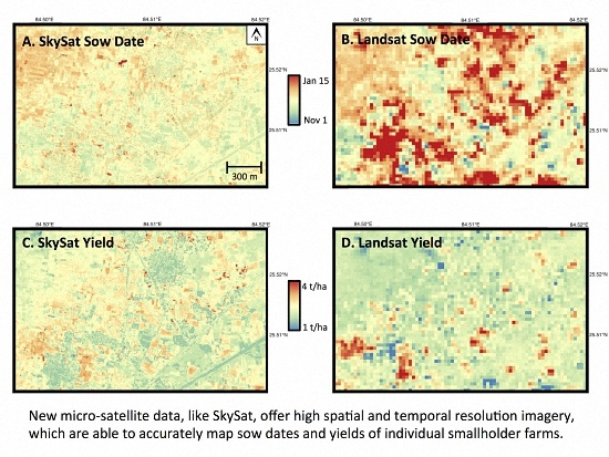
We obtained high-resolution SkySat imagery for an 8 × 16 km² region in Arrah district, Bihar, India (central coordinates: 25.47°N, 84.52°E) for the 2014–2015 and 2015–2016 winter growing seasons (Figure 1). This region is predominantly composed of smallholder agriculture, with farms covering over 80% of land area. There are three agricultural growing seasons in this region: the monsoon (kharif) season when a majority of farmers plant rice, the winter (rabi) season when most farmers plant wheat, and the summer (garmi) season when most fields remain fallow. We specifically focused this study on the winter season, which spans from early November to early April. There is significant heterogeneity in management practices, which leads to large variation in wheat yields across fields. Most farmers apply phosphate and nitrogen fertilizers, like DAP and urea, yet the amount applied varies from 20 kg to over 100 kg. There is also variation in the number of irrigations applied (typically one to three times) since irrigation is costly due to expensive diesel pumps. There is also a wide range in sow dates, spanning from 1 November to early January. Sow date has large impacts on yield, as crops that are sown late (typically from December onwards) face heat stress during grain filling, which leads to large reductions in yield [23,24]. Previous studies have shown that higher yields are associated with optimum sow dates [25,26], higher fertilizer use [27], and increased irrigation use [28,29]. Given the significant heterogeneity in yields across smallholder farms in this region, this site is ideal to examine how well micro-satellites can map field-level statistics. It is important to note that a large proportion of farmers intercrop mustard (varieties Rajendra Rye and RD 1002) with wheat (<10% of the total field), which potentially may lead to mixed spectral signatures within a given wheat field in our remote sensing analyses.

4. Approach

We used the following approach to address our two main objectives. First, to understand how calibration data type affects yield prediction accuracies, we collected crop cut and self-report data and created crop model data for our study region of interest (Section 5). We then used these data to develop algorithms that translate satellite vegetation indices to sow date and yield (Section 6.1), and assessed their accuracy in two ways (Section 6.2). We examined how predicted estimates compared to observed estimates, and how well yield predictions were able to capture known relationships between management variables and yield. Second, to identify how well high-resolution micro-satellite data perform compared to freely-available imagery, we predicted yields using 30 m Landsat imagery as well as SkySat imagery resampled to 30 m, which allows us to more fairly compare the amount of prediction accuracy lost due to coarser scale imagery alone (Section 6.3).

5. Data

5.1. SkySat Imagery

During the 2014–2015 growing season, six dates of mostly cloud-free imagery were acquired: 18 February, 11 March, 22 March, 23 March, 28 March, and 6 April. For the 2015–2016 growing season, five dates of mostly cloud-free imagery were acquired: 21 December, 3 January, 11 February, 16 March, and 4 April. We did not task specific image dates, and instead Terra Bella collected images depending on satellite availability, averaging approximately one image every two to three weeks. Imagery was not obtained during the first half of the wheat growing season in 2014–2015, but spanned the entire growing season in 2015–2016 (Figure 2). Terra Bella’s SkySat satellites collect optical multi-spectral imagery at 2-m resolution, which includes blue (0.450–0.515 nm), green (0.515–0.595 nm), red (0.605–0.695 nm), and near infra-red (0.740–0.900 nm) bands.

Pre-processing of Imagery: Nine separate tiles of imagery were collected for each date across our study region. There were radiometric differences between tiles collected along different paths by different detectors, particularly for the 2014–2015 imagery. To smooth these differences, we used ENVI seamless mosaicking with histogram matching across the entire scene. We did not use seamless mosaicking for the 2015–2016 imagery as these images were already mosaicked by Terra Bella. While some seams still remained, their visibility greatly reduced when we converted imagery to vegetation indices. To convert radiance to surface reflectance, we histogram matched each mosaicked SkySat image using histograms derived from Landsat surface reflectance imagery following simple approaches used in previous studies [30,31]. We selected the Landsat image that was closest in date to each of the SkySat images and subsetted it by the extent of our study region. If there was no Landsat image acquired within five days of a given SkySat date, we linearly interpolated between the histograms from the closest Landsat dates before and after the SkySat image was acquired. To geo-reference the SkySat imagery, we manually geo-referenced 300 locations in one SkySat image (11 March) using point locations obtained from Google Earth imagery. We then transformed this image using a thin plate spline and nearest neighbor resampling in QGIS. We automatically geo-referenced the remaining images to the manually geo-referenced image using image-to-image registration with an affine transformation in ENVI. Finally, we calculated the green chlorophyll vegetation index (GCVI; Equation (1)) for each image because previous studies have shown that GCVI has a fairly linear relationship with wheat leaf area index (LAI; [32]).

GCVI = (NIR/Green) − 1

(1)

Mask: To create a non-agriculture mask, we collected 297 points of different landcover classes across our SkySat region using i-Tree canopy software (http://www.itreetools.org/canopy), which relies on visual interpretation of high-resolution Google Earth imagery. We used 200 of these points as training data within a random forest model that used GCVI from all SkySat images to predict agriculture versus non-agriculture landcover classes. We validated the mask using the remaining 97 points, and obtained a user’s accuracy of 81.3% and a producer’s accuracy of 93.8% (Table S1). We did not develop a cloud mask because we used imagery that was mostly cloud free.

5.2. Landsat Imagery

To identify how well we could map smallholder yields and sow dates using SkySat imagery compared to Landsat imagery, we used Google Earth Engine to download all cloud-free Landsat Surface Reflectance imagery between 1 December and 15 April for the 2014–2015 and 2015–2016 growing seasons. Seven Landsat 7 and 8 images were available for 2014–2015 and 2015–2016 respectively. For 2014–2015, images were available for 1 February, 9 February, 17 February, 5 March, 13 March, 21 March and 29 March. For 2015–2016, images were available for 26 December, 11 January, 27 January, 12 February, 28 February, 8 March, and 16 March. We calculated GCVI for all images as previous studies have shown that GCVI has a fairly linear relationship with wheat LAI [32].

5.3. Crop Cut Data

Crop cut data were collected for 50 randomly selected fields across our study region in 2014–2015, and for 37 fields in 2015–2016. We visited these fields twice during the growing season to obtain necessary information. During the first visit in November, we collected GPS points at the four corners of one field for each farmer. We also asked farmers to report the sow date and wheat variety used in each field. During the second visit, which occurred at the time of harvest in April, we asked the same farmers questions about inputs into the system, including amount and type of fertilizer applied and number of irrigations used. We additionally recorded how heavily the field was lodged (defined as crops that have fallen over) on a scale of 1 (no lodging) to 10 (heavily lodged). In 2014–2015, we conducted crop cuts by selecting three 2 × 1 m² plots within each field, harvesting the crop from these sub-plots, and weighing the crop (biomass) and grain (yield) in the field. In 2015–2016, our team collected a total of twelve different crop cuts from each field because we were conducting a fertilizer experiment and had four sub-plot treatments in which we collected three crop cuts each. To calculate mean yield of a field, we averaged the yield values from all 2 × 1 m² crop cut plots within each field. We weighted lodged and unlodged plots equally because yields from these plots were fairly similar within a field. To link this crop cut information directly with SkySat imagery, we created polygons using the GPS locations of field boundaries collected for each field. When necessary, we manually adjusted each field’s polygon to ensure that it directly matched visible field boundaries in both SkySat and high-resolution Google Earth imagery.

5.4. Social Survey Self-Report Data

Social survey data were collected for 52 farmers in 2014–2015 and 29 farmers in 2015–2016 in mid-April, after wheat harvests had taken place. These farmers were independent of the ones that we visited to collect crop cut data. For each of these farmers, we visited one of his/her wheat fields in 2014–2015, conducted the survey while in the field, and collected GPS boundaries of each field. For the 2015–2016 season, we called farmers for whom we had collected field boundary data from during the previous year, and conducted the survey over the phone. We asked farmers to report management strategies used in the field, including amount of fertilizer and irrigation used, wheat cultivar planted, and sow date. Finally, we asked the farmers to report the wheat yield of each field. All self-report yield measures were converted to kilograms per hectare to ensure these data were comparable to the crop cut data.

5.5. Crop Model Data

Previous work has shown that crop model outputs may be used to develop and calibrate models that translate satellite vegetation indices to yield [16]. We use similar methods to those derived in Lobell et al. (2015) to test whether this approach, called SCYM, may accurately map the yields of smallholder farms. With this method, a suite of crop models are run that encompass variation in management across the study region, and then daily LAI outputs from the crop models are converted into daily vegetation indices (VIs) using field-tested and calibrated equations that relate VIs to crop LAI (e.g., [32]). We then create linear models where we regress simulated yield on simulated VIs for the dates that we have satellite imagery. For this study, we used the APSIM wheat crop model [33], which we parameterized using a range of management variables obtained through our surveys with farmers and from previous literature (specific parameters and references are listed in Table S2) as well as crop parameters for the most prevalent wheat variety, PBW-343 [34,35]. We also input daily weather data, including radiation as well as minimum and maximum temperature from NASA POWER (Prediction of Worldwide Energy Resource; http://power.larc.nasa.gov) and rainfall from CHIRPS (Climate Hazards Group InfraRed Precipitation with Station data; http://chg.geog.ucsb.edu/data/chirps/). We compared NASA POWER estimates of temperature with station data, and found that NASA POWER mean temperature is typically a few degrees warmer. Thus, we used the mean of MODIS LST daytime and nighttime temperature, which has been shown to accurately measure mean temperature [36,37] to correct the mean of NASA POWER temperature estimates. We converted daily wheat LAI simulations to GCVI using Equation (2), which was derived from subfield-level estimates [32].

LAI = −0.003 × GCVI² + 0.64 × GCVI − 0.37

(2)

6. Methods

We calculated wheat yield from SkySat imagery using three different datasets to parameterize linear models. The first method used crop cut data, the second method used self-report data, and the third method used outputs from our crop model simulations. In the case of sow date, only two types of data were used, self-reports and outputs from crop models. However, since there was temporal variation in when the self-reports were collected, with self-report sow date collected close to the timing of planting in our crop cut survey but at the end of the growing season in the self-report survey, we parameterized two separate models using these two datasets. The difference in performance between these two datasets can help identify whether the timing of surveys has an effect on self-report accuracy. Model parameterization and validation are described below.

6.1. Model Parameterization

We developed and calibrated linear models because the relationship between our outcome variables of interest (sow date and yield) and GCVI for our crop cut plots was predominantly linear (Figures S1 and S2). We also observed that GCVI and yield were not linearly related in fields that were heavily lodged, likely because these plots had low yields regardless of early season GCVI. We thus removed fields that were heavily lodged (lodging score > 6) from our analyses since we would not expect a relationship between early season GCVI and final yield. 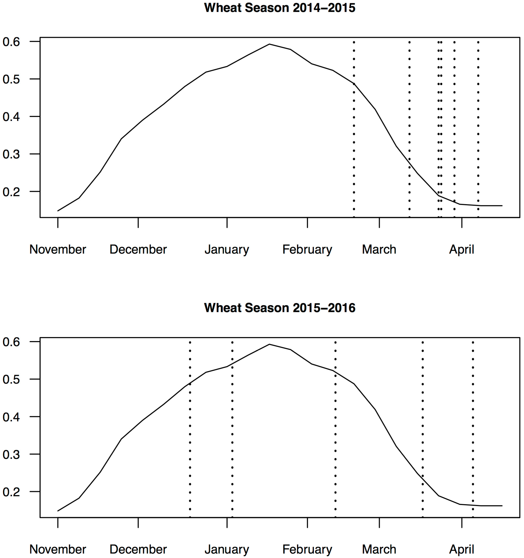To reduce the chance of model overfitting, we examined the correlation between GCVI across all dates (Table S3). Since 22 March and 23 March in the 2014–2015 imagery were highly correlated (R > 0.92), we omit 23 March from all analyses. We also examined the phenologies of GCVI through time for each of our crop cut fields (Figure S3), and since early sown and higher yielding plots had higher maximum GCVI values than late sown and low yielding plots, we consider the maximum GCVI value attained across all SkySat image dates as a predictor in our models.

We developed linear models that used all possible image dates. This is because our analyses suggested that models that used all image dates had the highest R² for both yield and sow date predictions (see Results, Section 7). However, for crop model parameterized models, we restricted our analysis to only include images before mid-March. This is because wheat phenologies in our crop model simulations matured and senesced one month earlier than observed phenologies, resulting in a mismatch between our observed and crop model phenologies after mid-March. This mismatch has been well documented in previous studies [35], especially for late sown wheat in north-western India, and this has been identified as a weakness in the APSIM model and an important area for future research [38].

6.2. Validation of Models

We validated sow date and yield estimates for the crop cut, self-report, and crop model parameterized models in two ways. First, we applied coefficient values derived from our linear models to the GCVIs associated with the crop cut polygons. We used the crop cut data for validation because we believe these data to be our most accurate measure for yields. We also used the sow date data collected in the crop cut survey as validation for sow dates, as we hypothesize that farmers will report sow date more accurately closer to the timing of planting. We then examined R² and RMSE between predicted sow dates and yields from each of the best models and the observed sow dates and yields from our crop cut datasets.

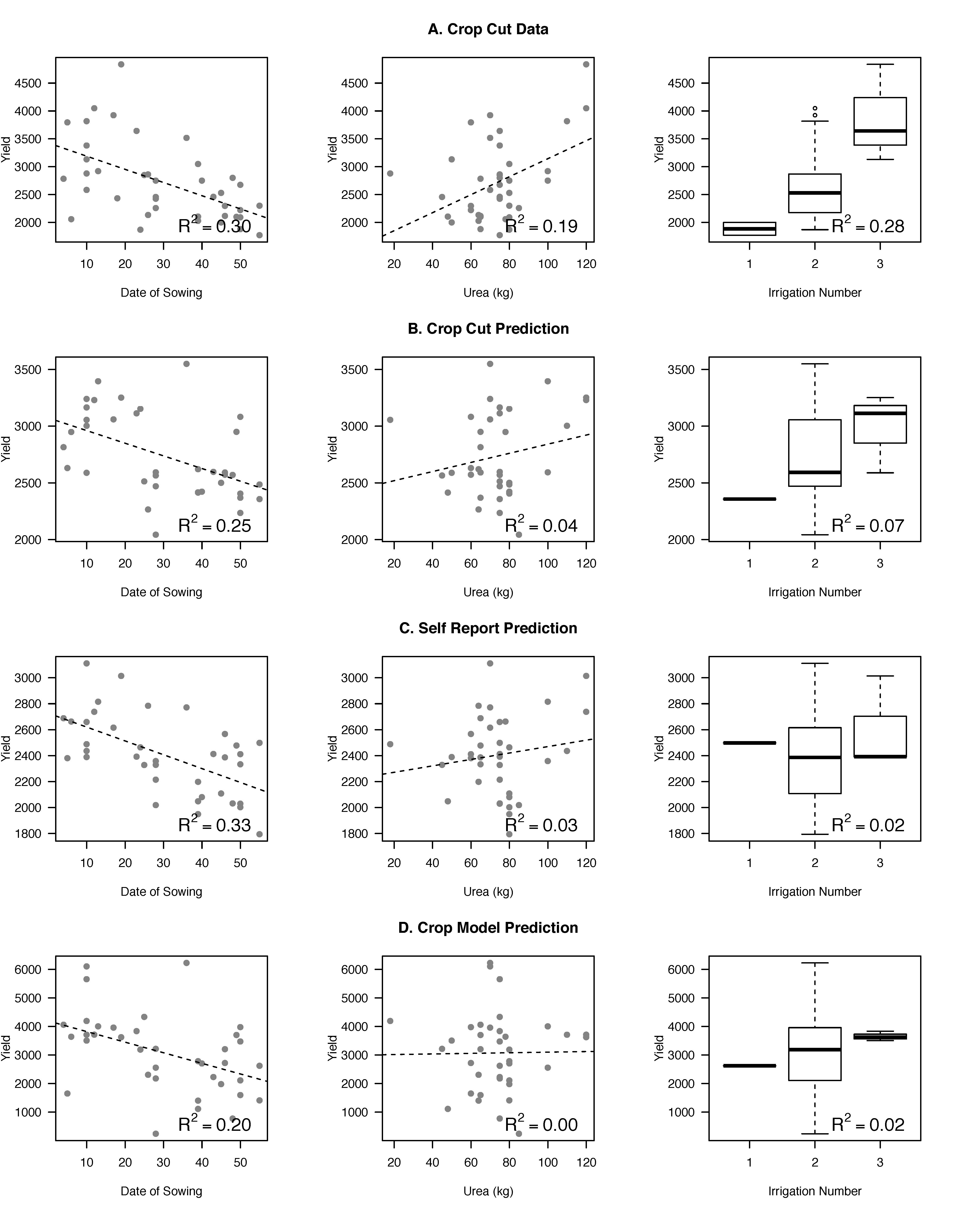
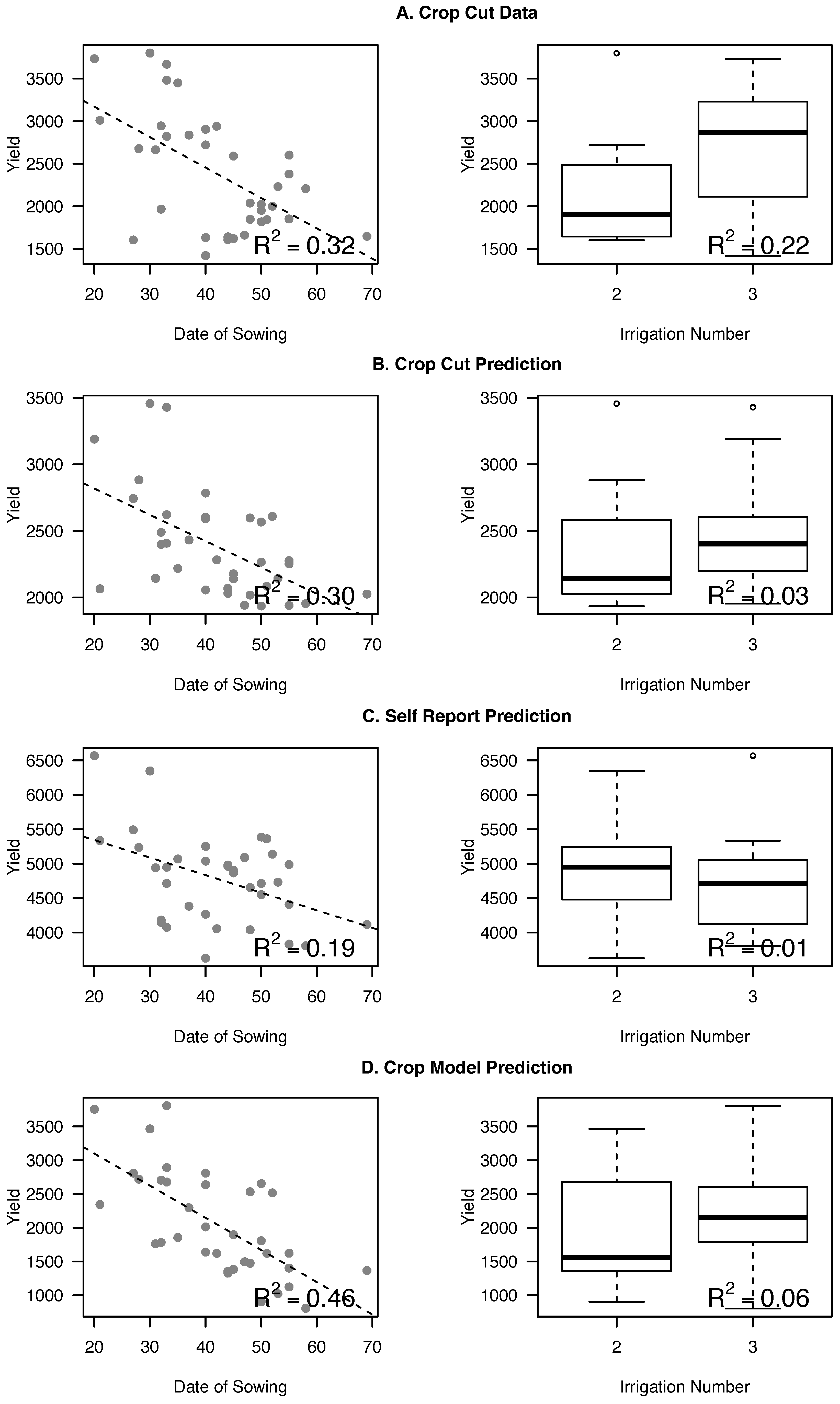
Our second test examined whether these models could produce yield estimates that can detect known signals between management variables and yield. Specifically, we examined the relationship between predicted yields and reported sow date, amount of fertilizer used (urea fertilizers), and number of irrigations applied. The closer these relationships matched associations observed between our crop cut yields and management variables, the better the satellite yield estimates were thought to be. We were unable to examine the relationship between fertilizer and yield in the 2015–2016 dataset because fertilizer was applied equally to all farms due to our fertilizer experiment, and therefore there was no variation in fertilizer to examine.

6.3. Comparison of SkySat and Landsat Imagery

To better identify the additional information gained from SkySat imagery compared to freely-available, coarser Landsat data, we conducted two additional analyses. First, we resampled SkySat imagery to 30 m to match the resolution of Landsat imagery, and redeveloped coefficient values for linear models that translate satellite vegetation indices to sow date or yield. By resampling SkySat data to 30 m, we specifically examine the predictive ability that is lost with coarser scale imagery. Second, we redeveloped coefficient values for linear models using all available cloud-free Landsat images within the 2014–2015 and 2015–2016 growing seasons. This analysis both examines the effect of coarser scale imagery as well as the effect of having increased temporal frequency of imagery on our sow date and yield estimates. This is because we had seven images available for both the 2014–2015 and 2015–2016 growing seasons compared to only five images available for SkySat in each season. For these analyses, we only develop models that use crop cut data as calibration data since this dataset was shown to result in the highest prediction accuracies. We did not examine how well Sentinel-2, a new freely available satellite product at 10 m resolution, performed because no data were available for 2014–2015 as this was prior to the satellite’s launch and only two cloud-free images were available for the 2015–2016 growing season.

7. Results

7.1. Prediction Accuracy

7.1.1. Sow Date Models

We use all available image dates for analyses because we find that prediction accuracies improve using all dates (Figure 3). For sow date, we compared predicted values derived from the crop cut, self-report, and crop model parameterized models with observed self-reports from the crop cut dataset (Figure 4 and Figure 5). For both years, we find that the crop cut parameterized model performs best, with an R² of 0.41 and an RMSE of 12.41 for the 2014–2015 season and an R² of 0.62 and an RMSE of 6.68 for the 2015–2016 season (Figure 4A and Figure 5A). This suggests that parameterizing models using self-report sow date from early in the growing season can lead to accurate predictions of sow date using satellite imagery. Considering the model parameterized with end-of-season self-report data (Figure 4B and Figure 5B), the model does less well, with an R² of 0.37 and RMSE of 14.57 in 2014–2015 and an R² of 0.0 and RMSE of 13.96 in 2015–2016. Most notably, our end-of-season self-report model rarely predicts sow dates before 30 November. This may be because no farmers report early sow dates (before 15 November) in the end-of-season self-report dataset. Finally, the models derived from crop models (Figure 4C and Figure 5C) perform worse than models parameterized with early-season self-reports and comparably to or better than models parameterized with end-of-season self-reports. The crop model parameterized algorithm resulted in an R² of 0.27 and RMSE of 25.56 in 2014–2015 and an R² of 0.40 and RMSE of 10.38 in 2015–2016.

7.1.2. Yield Models

We find that the model that uses crop cut data to parameterize a linear model most accurately maps field-level yield using satellite imagery (Figure 4D and Figure 5D, R² = 0.27, RMSE = 606.46 kg/ha in 2014–2015 and R² = 0.33, RMSE = 557.78 kg/ha in 2015–2016). In 2014–2015, where we only had access to late season imagery, this model does not predict many values above 3200 kg/ha, even though yields as high as 5000 kg/ha were observed. However, in 2015–2016 where we had access to imagery throughout the growing season, we were able to accurately predict higher yielding fields. The model parameterized using self-report yield data predicted yields less well but still explained a fair amount of variation, with an R² of 0.13 and RMSE of 738.47 in 2014–2015 and an R² of 0.06 and RMSE of 2532.35 in 2015–2016 (Figure 4E and Figure 5E). Finally, the crop model parameterized linear model performed better than the self-report model but worse than the crop cut model, with an R² of 0.15 and RMSE of 1296.12 in 2014–2015 and an R² of 0.27 and RMSE of 783.99 in 2015–2016 (Figure 4F and Figure 5F). This method appears to show variance in yield almost as well as our crop cut calibrated analyses in 2015–2016, when we have imagery throughout the growing season.

7.2. Ability to Capture Yield Responses to Management

Previous research has shown that wheat yields are strongly associated with management factors, including sow date [25,26], fertilizer inputs [27], and irrigation used [28,29]. Thus, one test of how well satellite data estimate yield is to see whether we can capture known relationships between management factors and predicted yields. To quantify the relationship between management factors and yield, we compared sow date, fertilizer input, and number of irrigations with mean yields measured using crop cut data. Consistent with prior work, we find that yield is positively associated with earlier sow date (R² of approximately 0.30), increased fertilizer use (R² of approximately 0.20), and increased number of irrigations (R² of approximately 0.25; Figure 6A and Figure 7A). We then compared yield predictions from satellite data with reported management variables to identify whether these relationships could be similarly captured. We find that the crop cut parameterized model does best in capturing management effects on yield (Figure 6B and Figure 7B), except for in the case of sow date where self-report models do better in 2014–2015 (Figure 6C) and crop model parameterized models do best in 2015–2016 (Figure 7D). Crop cut parameterized estimates capture the stronger effects of sow date and irrigation well, but have a weak association between fertilizer and yield. Considering the self-report models, estimated yields are able to capture the effect of sow date well, and the effect of fertilizer and irrigation weakly (Figure 6C and Figure 7C). This may be because this model resulted in a large amount of scatter around the one-to-one line for high yields (e.g., Figure 4E), which may make it difficult to capture the weaker effects of fertilizer and irrigation that rely on accurate prediction of high yields. Finally, the crop model estimated yield data were able to capture the effect of sow date on yields, but were unable to capture the effect of fertilizers and could only weakly capture the effects of irrigation on yield (Figure 6D and Figure 7D).

7.3. Comparison of SkySat and Landsat Imagery

We conducted two analyses to examine the value that SkySat data may add to sow date and yield predictions compared to freely-available, coarser scale Landsat data. When conducting this comparison, we only developed models that used crop cut data for calibration, as our previous results suggest that these calibration data result in the highest prediction accuracies. First, when we resampled existing SkySat data to 30 m resolution, we find that our ability to predict sow date and yield decreases, with R² dropping from 0.41 to 0.24 for sow date (Figure 8A) and 0.27 to 0.25 for yield in 2014–2015 (Figure 8B), and from 0.62 to 0.50 for sow date (Figure 8C) and 0.33 to 0.29 (Figure 8D) for yield in 2015–2016. In our second analyses, where we used all cloud-free Landsat imagery to develop sow date and yield prediction algorithms, we find that our ability to predict sow date and yield improves, likely due to the increased temporal frequency of available imagery. In 2014–2015, R² increased from 0.41 to 0.47 for sow date (Figure 8A) and 0.27 to 0.52 for yield (Figure 8B), and in 2015–2016 R² decreased from 0.62 to 0.56 for sow date (Figure 8C) and increased from 0.33 to 0.42 for yield (Figure 8D). To further examine whether this improvement in accuracy was due to increased temporal image availability or another factor related to the Landsat data, we conducted similar analyses where we restricted which Landsat image dates we used to only those that were close in date to our available SkySat imagery. With this analysis, we find that our ability to predict sow date and yield is more comparable to the accuracies achieved using SkySat imagery (R² of 0.33 and 0.53 for sow date in 2014–2015 and 2015–2016, respectively; R² of 0.28 and 0.40 for yield in 2014–2015 and 2015–2016, respectively). While Landsat analyses outperformed SkySat, likely due to increased temporal image availability, it is important to note that SkySat better allows one to map within and across field heterogeneity compared to Landsat due to its higher spatial resolution (Figure 9).

8. Discussion

This study adds to the growing body of literature that uses satellite imagery to monitor crop production of smallholder systems. This work is one of the first to examine how well new micro-satellite data can be used to map characteristics of individual fields, and assesses what types of calibration data can lead to the highest accuracies at low cost. Overall, we find that we were able to map sow date with high accuracies, particularly when using models that were parameterized with self-report sow dates collected close to the time of planting. While less accurate, we were able to capture the large range in sow dates across farms when using models parameterized with crop model simulations. We were also able to map yields fairly well, though the accuracy of yield predictions was not as high as that of sow date. When estimating yields, our models did best when parameterized with crop cut data. However, yields predicted using crop model simulations did almost as well in 2015–2016, when we had access to imagery throughout the growing season. These results suggest that new high-spatio temporal micro-satellite data can be used to map field-level characteristics of smallholder farms, but the accuracy of these estimates varies based on the type of data used to parameterize models that translate satellite vegetation indices to yield.

When deciding which data to use for calibration, it is important to consider not only prediction accuracy but also how easy it is to access training data given collection costs and data availability. While we find that models parameterized with crop cut data do best, it may be worth considering alternate lower-cost approaches to obtain training data. Considering sow date, models that were parameterized using crop models did almost as well as models that used self-reports (Figure 4C and Figure 5C). They were able to broadly capture the difference between early and late planted fields, and map the heterogeneity in sow date across farms. It may thus not be worth the cost and time needed to collect self-report sow date data since crop models that require no on-the-ground data do relatively well. Considering yield, while the crop cut parameterized model performed best, models parameterized with crop models were able to broadly distinguish between low versus high yielding plots (Figure 4E and Figure 5E) and did almost as well as crop cut calibrated models in 2015–2016 when we had imagery throughout the season. These models were able to capture the strongest associations between management factors, like sow date, and yield (Figure 6 and Figure 7). Interestingly, our social survey calibrated models performed worst on all measures of accuracy, though they were better in predicting sow date than yield. Our results suggest that models parameterized with lower cost data, like crop model simulations, may produce yield and sow date estimates that are accurate enough depending on the desired purpose of the study. For example, if one aims to distinguish between low versus high yielding plots, or to detect signals with large effect sizes, then yield estimates produced using lower-cost training data like crop models may do well.

While we were able to distinguish between low versus high yielding fields across all of our models, predictions were often biased. In the case of crop cut calibrated models, there is severe under-prediction of yields for high yielding fields (>3200 kg/ha) when we only had imagery towards the end of the growing season. This may have occurred because the linear relationship between GCVI and yield was weaker at the end of the growing season for fields with the highest yields (Figures S1 and S2), potentially due to mixed spectral signatures caused by intercropping wheat with mustard. Having access to imagery throughout the growing season reduced this problem, likely because the relationship between GCVI and yield is more linear for early season imagery. Yields were over-estimated considering self-report data, averaging 2000 kg/ha greater than observed yields in 2015–2016. This may be because self-report data were collected over the phone in this year, and since most farmers in this region own multiple plots, it is possible that farmers were less precise in giving estimates of the specific field for which we had GPS boundaries. There was over-prediction of yields considering crop models in 2014–2015, with predicted yields that were often 1000 kg/ha greater than observed yields. This is likely because of a mismatch between observed phenologies in our SkySat imagery versus crop model phenologies; crops matured and senesced about one month earlier in crop model simulations. Because of this, the highest prediction accuracies were obtained when using early season imagery (before March), when the observed and simulated phenologies were more closely aligned. Not having access to early season imagery in 2014–2015 likely led to greater inaccuracies in our yield estimates for that year. Future work should identify ways to better match simulated phenologies with observed phenologies for wheat in this region. Overall, while all predictions had some biases, they may not be problematic if one is more interested in yield variability across plots than knowing the absolute yield of a field.

We were also interested in identifying whether our prediction accuracy improved with increased temporal frequency of imagery. We find that our models improve with access to satellite imagery throughout the growing season (Figure 5). This is particularly true for sow date where R² improved from 0.41 to 0.62 when we had access to early season imagery. While yield estimates did not greatly improve with increased access to imagery, we were better able to capture the observed range in yields when we used early season imagery. Finally, our crop model calibrated algorithms performed significantly better when using early season imagery, with R² for both sow date and yield increasing by approximately 0.15. It is possible that our ability to predict both sow date and yield would improve even further if we had increased access to imagery throughout the growing season, with more than one image per month. This is suggested by previous studies that have found high accuracies in predicting yield with multi-temporal imagery that spans the length of the growing season [14,15,16] as well as our Landsat analyses (Figure 8). These previous studies were able to predict yields with R² ranging from 0.21 to 0.64 (e.g., [14,15,16]), and our results are thus comparable to accuracies achieved in previous studies using other satellite data and on-the-ground calibration data. As more high-resolution satellite data become available, future work will examine how much prediction accuracies further improve with near weekly or bi-weekly imagery.

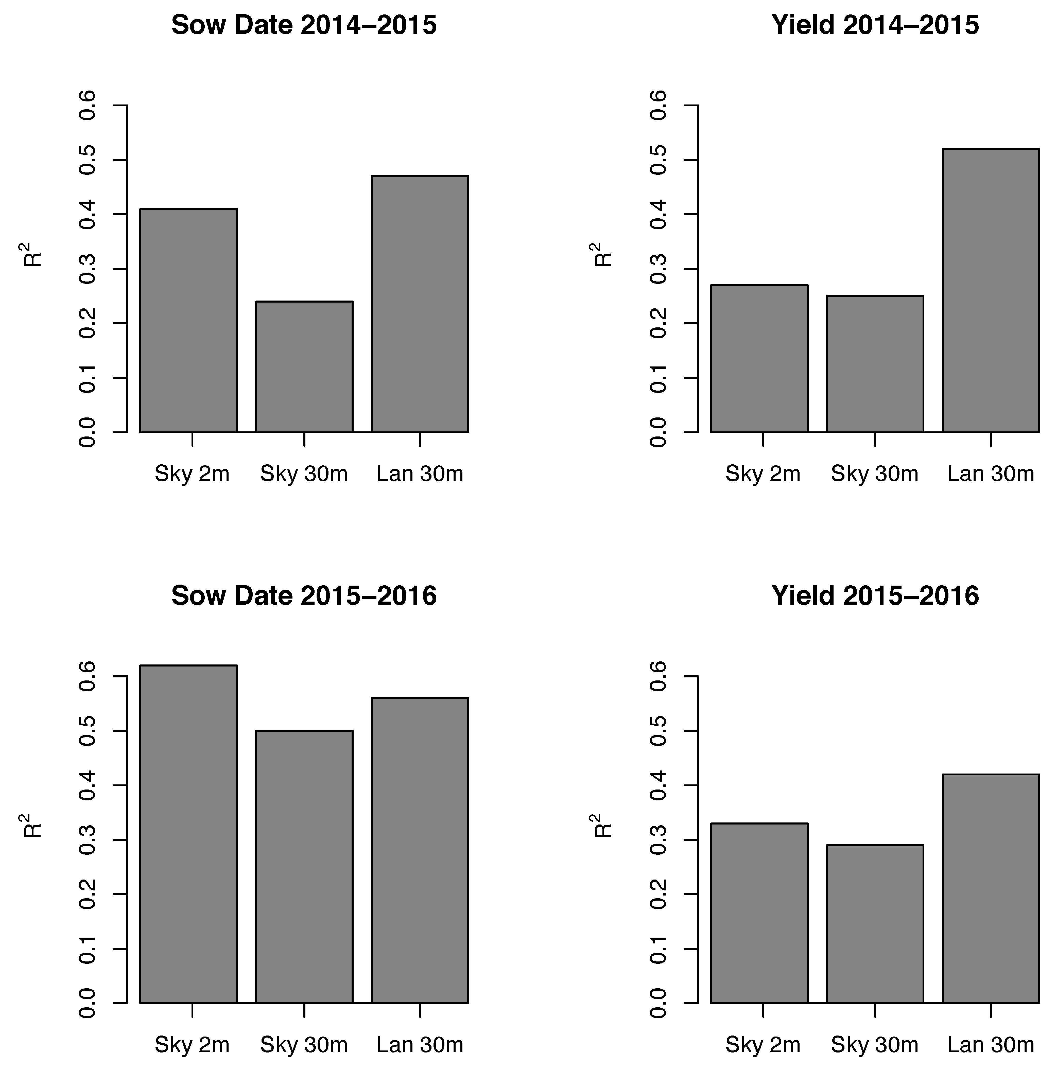
Considering the relative benefit of using high-resolution SkySat imagery compared to freely-available, coarser Landsat imagery, we find that accuracies for predicting sow date and yield decrease when SkySat imagery is resampled to match the spatial resolution of Landsat (Figure 8). This suggests that high-resolution imagery results in more accurate field-level predictions, likely by reducing the effect of mixed pixels caused by small field sizes and heterogeneous management across farms. 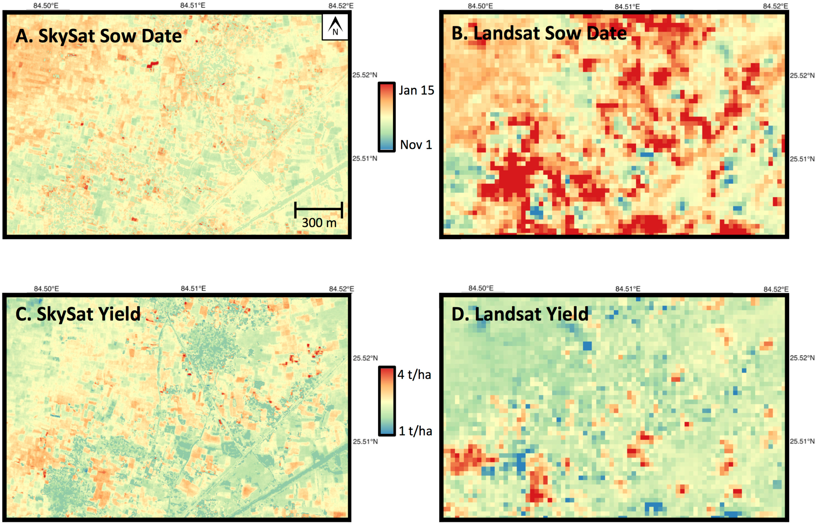We find that we produce more accurate yield estimates but comparable sow date estimates to those produced using SkySat imagery when we use all-available Landsat imagery (Figure 8). It is likely these improved accuracies are driven by the increased temporal frequency of Landsat, as seven Landat images were available versus five for SkySat. Despite these improved accuracies in mapping field-level yields, a significant amount of spatial information is lost when using coarser Landsat imagery. With high-resolution SkySat data, we captured within field heterogeneity, which is often as large as across field variation (Figure 9). These tradeoffs suggest that whether one should use micro-satellite data or current, freely-available imagery depends on the goals of the study. Landsat currently offers better temporal coverage, and our results suggest that this increased temporal frequency is particularly important for mapping field-level yields. However, SkySat imagery offer the ability to examine within and across field yield variation that is not possible using coarser resolution Landsat data.

Future work should further explore several uncertainties in this study. First, it is unclear how widely the algorithms that we developed to map yield and sow date can be applied. For example, future work should examine whether the same models can be used across larger spatial scales and across multiple years. Furthermore, we were unable to partition the amount of predictive error that was due to radiometric correction issues with SkySat; it is possible that future studies may be able to achieve higher predictive accuracies once micro-satellite data are better radiometrically calibrated and mosaicked.

9. Conclusions

This study shows that high spatio-temporal micro-satellite data can be used to map individual field-level characteristics of smallholder farms with significant accuracy, capturing roughly one-half and one-third of the variation in field-measured sow date and yields, respectively, when parameterized with field measures. Considering calibration datasets, this study highlights that while the best prediction accuracies can be achieved using on-the-ground crop cut data, we are able to produce accurate estimates of yield using lower cost parameterization data, like crop model simulations that require no on-the-ground data. While yield estimates produced using these lower-cost data have reduced prediction accuracy compared to crop cut models, they are still able to differentiate between low versus high yield fields and are able to capture the strongest known relationships between management variables and yield. This suggests that crop model simulations and the SCYM approach [16] may be a viable way to map agricultural production with little to no ground data, even in heterogeneous smallholder systems. Finally, we find that accuracies for predicting smallholder sow date and yield can be improved when using imagery that spans the entire growing season, and likely will be improved further as the temporal frequency of imagery increases. This study has uniquely added to the growing body of literature that aims to map crop production statistics of smallholder farms. Specifically, this study is one of the first to evaluate how well new micro-satellite data can be used to map smallholder characteristics, and it also examines what type of calibration data can produce accurate results at low cost. The results of this study suggest that new micro-satellite data are a viable product to map field-level farm characteristics, and their utility will only improve as these satellites develop increased temporal frequency throughout the growing season.

References

1. Schmidhuber, J.; Tubiello, F.N. Global food security under climate change. Proc. Natl. Acad. Sci. USA 2007, 104, 19703–19708. [Google Scholar] [CrossRef] [PubMed]
2. Lobell, D.B.; Burke, M.B.; Tebaldi, C.; Mastrandrea, M.D.; Falcon, W.P.; Naylor, R.L. Prioritizing climate change adaptation needs for food security in 2030. Science 2008, 319, 607–610. [Google Scholar] [CrossRef] [PubMed]
3. Stocking, M.A. Tropical soils and food security: The next 50 years. Science 2003, 302, 1356–1359. [Google Scholar] [CrossRef] [PubMed]
4. Godfray, H.C.J.; Beddington, J.R.; Crute, I.R.; Haddad, L.; Lawrence, D.; Muir, J.F.; Pretty, J.; Robinson, S.; Thomas, S.M.; Toulmin, C. Food security: The challenge of feeding 9 billion people. Science 2010, 327, 812–818. [Google Scholar] [CrossRef] [PubMed]
5. Morton, J.F. The impact of climate change on smallholder and subsistence agriculture. Proc. Natl. Acad. Sci. USA 2007, 104, 19680–19685. [Google Scholar] [CrossRef] [PubMed]
6. Lobell, D.B.; Schlenker, W.; Costa-Roberts, J. Climate trends and global crop production since 1980. Science 2011, 333, 616–620. [Google Scholar] [CrossRef] [PubMed]
7. Carfagna, E.; Gallego, F.J. Using remote sensing for agricultural statistics. Int. Stat. Rev. 2005, 73, 389–404. [Google Scholar] [CrossRef]
8. Atzberger, C. Advances in remote sensing of agriculture: Context description, existing operational monitoring systems and major information needs. Remote Sens. 2013, 5, 949–981. [Google Scholar] [CrossRef]
9. Bastiaanssen, W.G.M.; Ali, S. A new crop yield forecasting model based on satellite measurements applied across the Indus Basin, Pakistan. Agric. Ecosyst. Environ. 2003, 94, 321–340. [Google Scholar] [CrossRef]
10. Jain, M.; Mondal, P.; DeFries, R.S.; Small, C. Mapping cropping intensity of smallholder farms: A comparison of methods using multiple sensors. Remote Sens. Environ. 2013, 134, 210–223. [Google Scholar] [CrossRef]
11. Dobermann, A.; Ping, J.L. Geostatistical integration of yield monitor data and remote sensing improves yield maps. Agron. J. 2004, 96, 285–297. [Google Scholar] [CrossRef]
12. Yang, C.; Everitt, J.H.; Bradford, J.M. Comparison of QuickBird satellite imagery and airborne imagery for mapping grain sorghum yield patterns. Precis. Agric. 2006, 7, 33–44. [Google Scholar] [CrossRef]
13. Serrano, L.; Filella, I.; Penuelas, J. Remote sensing of biomass and yield of winter wheat under different nitrogen supplies. Crop Sci. 2000, 40, 723–731. [Google Scholar] [CrossRef]
14. Labus, M.P.; Nielsen, G.A.; Lawrence, R.L.; Engel, R.; Long, D.S. Wheat yield estimates using multi-temporal NDVI satellite imagery. Int. J. Remote Sens. 2002, 23, 4169–4180. [Google Scholar] [CrossRef]
15. Morel, J.; Todoroff, P.; Bégué, A.; Bury, A.; Martiné, J.-F.; Petit, M. Toward a satellite-based system of sugarcane yield estimation and forecasting in smallholder farming conditions: A case study on Reunion Island. Remote Sens. 2014, 6, 6620–6635. [Google Scholar] [CrossRef]
16. Lobell, D.B.; Thau, D.; Seifert, C.; Engle, E.; Little, B. A scalable satellite-based crop yield mapper. Remote Sens. Environ. 2015, 164, 324–333. [Google Scholar] [CrossRef]
17. Fermont, A.; Benson, T. Estimating Yield of Food Crops Grown by Smallholder Farmers; IFPRI Discussion Paper; IFPRI: Washington, DC, USA, 2011. [Google Scholar]
18. Quarmby, N.A.; Milnes, M.; Hindle, T.L. The use of multi-temporal NDVI measurements from AVHRR data for crop yield estimation and prediction. Int. J. Remote Sens. 1993, 14, 199–210. [Google Scholar] [CrossRef]
19. Murthy, C.S.; Thiruvengadachari, S.; Raju, P.V.; Jonna, S. Improved ground sampling and crop yield estimation using satellite data. Int. J. Remote Sens. 1996, 17, 945–956. [Google Scholar] [CrossRef]
20. Shanahan, J.F.; Schepers, J.S.; Francis, D.D.; Varvel, G.E.; Wilhelm, W.W.; Tringe, J.M.; Schlemmer, M.R.; Major, D.J. Use of remote-sensing imagery to estimate corn grain yield. Agron. J. 2001, 93, 583–589. [Google Scholar] [CrossRef]
21. Carletto, C.; Jolliffe, D.; Banerjee, R. The Emperor Has No Data! Agricultural Statistics in Sub-Saharan Africa; World Bank Working Paper; World Bank: Washington, DC, USA, 2013. [Google Scholar]
22. Ladha, J.K.; Dawe, D.; Pathak, H.; Padre, A.T.; Yadav, R.L.; Singh, B.; Singh, Y.; Singh, Y.; Singh, P.; Kundu, A.L.; et al. How extensive are yield declines in long-term rice-wheat experiments in Asia? Field Crop. Res. 2003, 81, 159–180. [Google Scholar] [CrossRef]
23. Asseng, S.; Foster, I.; Turner, N.C. The impact of temperature variability on wheat yields. Glob. Chang. Biol. 2011, 17, 997–1012. [Google Scholar] [CrossRef]
24. Gourdji, S.M.; Mathews, K.L.; Reynolds, M.; Crossa, J.; Lobell, D.B. An assessment of wheat yield sensitivity and breeding gains in hot environments. Proc. R. Soc. B Biol. Sci. 2012, 280, 20122190. [Google Scholar] [CrossRef] [PubMed]
25. Ortiz-Monasterio R, J.I.; Dhillon, S.S.; Fischer, R.A. Date of sowing effects on grain yield and yield components of irrigated spring wheat cultivars and relationships with radiation and temperature in Ludhiana, India. Field Crop. Res. 1994, 37, 169–184. [Google Scholar] [CrossRef]
26. Erenstein, O.; Laxmi, V. Zero tillage impacts in India’s rice-wheat systems: A review. Soil Tillage Res. 2008, 100, 1–14. [Google Scholar] [CrossRef]
27. Yadav, R.L. Assessing on-farm efficiency and economics of fertilizer N, P and K in rice wheat systems of India. Field Crop. Res. 2003, 81, 39–51. [Google Scholar] [CrossRef]
28. Singh, A.K.; Jain, G.L. Effect of sowing time, irrigation and nitrogen on grain yield and quality of duram wheat (Triticum durum). Indian J. Agric. Sci. 2000, 70, 532–533. [Google Scholar]
29. Fishman, R.M. Climate change, rainfall variability, and adaptation through irrigation: Evidence from Indian agriculture. Unpublished work. 2012. [Google Scholar]
30. Horn, B.K.P.; Woodham, R.J. Destriping LANDSAT MSS images by Histogram Modification. Comput. Graph. Image Porcess. 1979, 10, 69–83. [Google Scholar] [CrossRef]
31. Weinreb, M.P.; Xie, R.; Lienesch, J.H.; Crosby, D.S. Destriping GOES images by matching empirical distribution functions. Remote Sens. Environ. 1989, 29, 185–195. [Google Scholar] [CrossRef]
32. Nguy-Robertson, A.L.; Peng, Y.; Gitelson, A.A.; Arkebauer, T.J.; Pimstein, A.; Herrmann, I.; Karnieli, A.; Rundquist, D.C.; Bonfil, D.J. Estimating green LAI in four crops: Potential of determining optimal spectral bands for a universal algorithm. Agric. For. Meteorol. 2014, 192–193, 140–148. [Google Scholar] [CrossRef]
33. Holzworth, D.P.; Huth, N.I.; deVoil, P.G.; Zurcher, E.J.; Herrmann, N.I.; McLean, G.; Chenu, K.; van Oosterom, E.J.; Snow, V.; Murphy, C.; et al. APSIM—Evolution towards a new generation of agricultural systems simulation. Environ. Model. Softw. 2014, 62, 327–350. [Google Scholar] [CrossRef]
34. Balwinder-Singh; Gaydon, D.S.; Humphreys, E.; Eberbach, P.L. The effects of mulch and irrigation management on wheat in Punjab, India—Evaluation of the APSIM model. Field Crop. Res. 2011, 124, 1–13. [Google Scholar] [CrossRef]
35. Balwinder-Singh; Humphreys, E.; Sudhir-Yadav; Gaydon, D.S. Options for increasing the productivity of the rice-wheat system of north-west India while reducing groundwater depletion. Part 1. Rice variety duration, sowing date and inclusion of mungbean. Field Crop. Res. 2015, 173, 68–80. [Google Scholar]
36. Vancutsem, C.; Ceccato, P.; Dinku, T.; Connor, S.J. Evaluation of MODIS land surface temperature data to estimate air temperature in different ecosystems over Africa. Remote Sens. Environ. 2010, 114, 449–465. [Google Scholar] [CrossRef]
37. Zhu, W.; Lű, A.; Jia, S. Estimation of daily maximum and minimum air temperature using MODIS land surface temperature products. Remote Sens. Environ. 2013, 130, 62–73. [Google Scholar] [CrossRef]
38. Gaydon, D.S.; Balwinder-Singh; Wang, E.; Poulton, P.L.; Ahmad, B.; Ahmed, F.; Akhter, S.; Ali, I.; Amarasingha, R.; Chaki, A.K.; et al. Evaluation of the APSIM model in cropping systems of Asia. Field Crop. Res. 2016. under review. [Google Scholar]
Figure 1. Study region in Arrah district, Bihar, India. The study region extent is highlighted by the dark blue rectangle. The state boundary of Bihar is highlighted in white.
Remotesensing 08 00860 g001
Figure 2. Graph showing the phenology of one example wheat pixel using 16-day MODIS Terra imagery in our study region. Dates when SkySat images were available are highlighted with vertical dashed lines.
Remotesensing 08 00860 g002
Figure 3. Change in R2 by adding an additional image date for the 2015–2016 study season using crop cuts as calibration data. Each image date was added from most to least important based on variable importance measures from random forest analyses.
Remotesensing 08 00860 g003
Figure 4. Sow date and yield prediction accuracies using 2014–2015 imagery. Predicted versus observed sow dates using: the crop cut parameterized model (A); the self-report parameterized model (B); and the crop model parameterized model (C). Predicted versus observed yields using: the crop cut parameterized model (D); the self-report parameterized model (E); and the crop model parameterized model (F). The one to one line is highlighted with a dashed line, and R2 and RMSE for each analysis are reported.
Remotesensing 08 00860 g004
Figure 5. Sow date and yield prediction accuracies using 2015–2016 imagery. Predicted versus observed sow dates using: the crop cut parameterized model (A); the self-report parameterized model (B); and the crop model parameterized model (C). Predicted versus observed yields using: the crop cut parameterized model (D); the self-report parameterized model (E); and the crop model parameterized model (F). The one to one line is highlighted with a dashed line, and R2 and RMSE for each analysis are reported.
Remotesensing 08 00860 g005
Figure 6. The relationship between yields and sow date, urea fertilizer added, and number of irrigations for 2014–2015 data: (A) known relationships between these management variables and yield as measured using the crop cut yield data collected in the field; (B) relationships with yield estimates using the crop cut parameterized model; (C) relationships with yield estimates using the self-report model; and (D) relationships with yield estimates using the crop model parameterized model. R2 between management variables and yield are highlighted in each graph.
Remotesensing 08 00860 g006
Figure 7. The relationship between yields, sow date, and urea fertilizer added for 2015–2016 data: (A) known relationships between these management variables and yield as measured using the crop cut yield data collected in the field; (B) relationships with yield estimates using the crop cut parameterized model; (C) relationships with yield estimates using the self-report model; and (D) relationships with yield estimates using the crop model parameterized model. R2 between management variables and yield are highlighted in each graph.
Remotesensing 08 00860 g007
Figure 8. R2 for all-date models predicting sow date (A) and yield (B) in 2014–2015 and sow date (C) and yield (D) in 2015–2016 using either the original SkySat data (Sky 2 m), SkySat data resampled to 30 m (Sky 30 m), or Landsat data (Lan 30 m). Five images are used for all SkySat analyses, while seven are used for Landsat analyses.
Remotesensing 08 00860 g008
Figure 9. Predicted sow date using SkySat (A) and Landsat (B) as well as predicted yields using SkySat (C) and Landsat (D). All predictions were done using crop cut data for calibration. SkySat predictions allow one to examine across and within field variability, which cannot be observed using Landsat predictions.
Remotesensing 08 00860 g009