Guidance Index for Shallow Landslide Hazard Analysis

Abstract

Rainfall-induced shallow landslides are one of the most frequent hazards on slanted terrains. Intense storms with high-intensity and long-duration rainfall have high potential to trigger rapidly moving soil masses due to changes in pore water pressure and seepage forces. Nevertheless, regardless of the intensity and/or duration of the rainfall, shallow landslides are influenced by antecedent soil moisture conditions. As of this day, no system exists that dynamically interrelates these two factors on large scales. This work introduces a Shallow Landslide Index (SLI) as the first implementation of antecedent soil moisture conditions for the hazard analysis of shallow rainfall-induced landslides. The proposed mathematical algorithm is built using a logistic regression method that systematically learns from a comprehensive landslide inventory. Initially, root-soil moisture and rainfall measurements modeled from AMSR-E and TRMM respectively, are used as proxies to develop the index. The input dataset is randomly divided into training and verification sets using the Hold-Out method. Validation results indicate that the best-fit model predicts the highest number of cases correctly at 93.2% accuracy. Consecutively, as AMSR-E and TRMM stopped working in October 2011 and April 2015 respectively, root-soil moisture and rainfall measurements modeled by SMAP and GPM are used to develop models that calculate the SLI for 10, 7, and 3 days. The resulting models indicate a strong relationship (78.7%, 79.6%, and 76.8% respectively) between the predictors and the predicted value. The results also highlight important remaining challenges such as adequate information for algorithm functionality and satellite based data reliability. Nevertheless, the experimental system can potentially be used as a dynamic indicator of the total amount of antecedent moisture and rainfall (for a given duration of time) needed to trigger a shallow landslide in a susceptible area. It is indicated that the SLI algorithm can be re-built for other regions where deterministic studies are not feasible. This represents a significant step towards rainfall-induced shallow landslide hazard readiness.

1. Introduction

Landslides are considered to be dependent on the complex interaction of several static and dynamic factors. Surface characteristics such as geomorphology, soil, land cover, and geology are considered static, and factors that trigger the mass movement are considered to be dynamic [1,2,3]. Though multiple factors play a significant role in landslide occurrence, it is usually a single dynamic factor that becomes the trigger element of a landslide event [4]. Landslides that are triggered by rainfall are known for their shallow depth between 0.3 and 2 m in thickness and for their great potential to cause significant damage to human beings and property [1,4].

The study of shallow rainfall-induced landslides is particularly important as global climate changes are expected to influence regional precipitation patterns such as precipitation intensity and distribution [5,6]. Storms with high-intensity and long-duration rainfall have high potential to trigger rapidly moving soil masses due to changes in pore water pressure and seepage forces [7,8,9]. The literature describes two distinctive failure mechanisms for shallow rainfall-induced landslides. The first mechanism is based on the reduction of hydraulic conductivity in the weathering profile and the increase of its density with depth [4,10,11]. In this scenario, the percolation rate lags behind the rainfall rate, creating a perched water flow that is parallel to the slope. The undrained conditions lead to increase pore pressure and to the reduction of shear strength which results in slope failure [4]. The second mechanism describes the advancement of water from the surface of the slope while the material is still unsaturated. At this point, reduced suction results in failure in the form a rigid mass [4,11].

Rainfall events can be analyzed to define statistical or empirical correlations between rainfall’s intensity and duration to shallow landslide occurrence. This relationship is often expressed in a mathematical law that defines a rainfall threshold, which is based on the assumption that past relationships between rain and landslides are valid for the future. When conditions exceed the threshold, landslides should be expected [12]. Caine (1980) described the relationship linking rainfall intensity (I) and duration (D) as a power law ($I=a{D}^{-b}$, where I is the rainfall mean intensity, D is the duration of the rainfall event, $\alpha$ is the scaling constant, and b defines the slope).

Following this methodology, several studies around the world have focused their attention on working with rainfall thresholds to define or assess the prediction of shallow landslide occurrence [13,14,15,16,17,18,19,20]. Nevertheless, these rainfall thresholds do not consider antecedent soil moisture conditions on the ground. It is well established that even though rainfall is a triggering factor, it is not the sole culprit of slope instability as increased pore pressure generates shallow landslides [4]. Antecedent soil moisture conditions significantly influence shallow landslide initiation as the spatial distribution of moisture content in the soil and pore water pressure controls the dynamics of shear strength and effective stress. Water pressure within the porosity of the soil expands the pore space and reduces the frictional forces between soil particles triggering slope instability [9].

Furthermore, physically-based models that simulate the soil’s hydrological dynamics after rainfall have demonstrated that rainfall alone is not adequate to identify instability and that antecedent soil moisture conditions are substantial in the generation of this phenomenon [21,22,23,24]. Rainfall intensity-duration thresholds can be indicators of precipitation as a precursor of shallow landslide activity, but antecedent soil moisture conditions significantly influence shallow landslide initiation as gravity drainage becomes negligible when soil water content falls below the soil's field capacity [25]. Moreover, the spatial distribution of moisture content in the soil and pore water pressure control the dynamics of shear strength and effective stress, water pressure within the porosity of the soil expands the pore space and reduces the frictional forces between soil particles triggering slope instability [9].

Additionally, precipitation thresholds of rainfall and duration do not provide information about the soil wetness profile with depth. Regardless of the intensity-duration of the rainfall, shallow landslides are influenced by antecedent soil moisture conditions. For example, a substantial precipitation episode within a dry period is not likely to trigger shallow landslides any less than a low-intensity rainfall would within a wet period [26]. Furthermore, damp antecedent conditions are likely to cause greater debris flow of greater magnitude during or following a given rainstorm [19]. As shallow landslide hazards are related to the interaction of static conditions and the temporal distribution of triggering factors, defining a methodology that accounts for “pre-event” or antecedent soil moisture conditions can significantly improve the accuracy of rainfall-triggered shallow landslide hazard modeling.

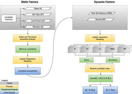
The present study centers on shallow rainfall-triggered landslides as described in the first failure mechanism. Machine-learning methods are used to develop a mathematical algorithm that presents the minimum amount of antecedent soil moisture and rainfall accumulation that results in a shallow landslide event. This leads to the development of an index value that serves as guidance within susceptible areas in the Continental United States.

Susceptible areas that represent “where” shallow landslides happen are defined utilizing a comprehensive landslide inventory and static factors as defined in Hong (2007) and Cullen (2016). “When” shallow landslides happen, is defined as the space-time variation of antecedent soil moisture and rainfall distribution. Although the system is built to assist stakeholders to foresee potential shallow landslide areas days in advance, factors that represent temporal-spatial vulnerability such as “who” will be affected are not considered in this work. Nevertheless, it is expected that the system can facilitate the decision-making processes to assess risk.

2. Materials and Methods

Rainfall-induced shallow landslides are the result of static and dynamic factors. The processes utilized to deal with the challenges that arise when dealing with static factors are described in Cullen (2016) where buffer and threshold techniques that help minimize uncertainties of slope representation at large extents are presented [3]. The current work introduces dynamic factors and machine-learning methods to develop a mathematical algorithm that relates remotely sensed antecedent soil moisture conditions to rainfall. Figure 1 shows the workflow where static and dynamic factors are correlated to develop the index.

2.1. Static Factors

The selection of static factors in the study of landslides is highly dependent on the scale of the analysis, the failure mechanism, and the landslide type, there is not a universal list of static factors [27]. Analysis over large domains can represent large computational power and time; well-planned selection of variables is imperative and dependent on the failure mechanism and the landslide type. C.J. van Western (2008) highlighted the most significant static factors in determining landslide susceptibility at regional scales. Nevertheless, some factors are more relevant in the study of rainfall-triggered landslides over a large domain than others. Hong (2007) established that the primary static factors influencing shallow landslides are slope, soil type, and land cover [1]. Cullen (2016) experimented with such variables in a logistic regression model and explains that the likelihood-ratio determines the relevance of all variables. The study concludes that the selected variables explain a high percent of the variance of the dependent variable at a 97.2% accuracy rate [3].

The static factors involved in this research are derived from Hong (2007) and from the initial analysis in Cullen (2016). The ASTER Global Digital Elevation Model (GDEM2) is used in this work as a topographic representation of the study area. Soil type was obtained from the Harmonize World Soil Database Version (HWSD) 1.2. This dataset combines existing regional and national updates of soil information from around the world and incorporates them into the Food and Agriculture Organization of the United Nations (FAO-UNESCO) Soil Map of the World at a 1 km resolution. Land cover was retrieved from the FAO Global Land Cover-SHARE database at 1 km resolution. This dataset integrates local and global land cover information. Local information is derived from datasets such as Africover and Corine LC and global data is derived from the Moderate-resolution Imagine Spectroradiometer (MODIS) Vegetation Continuous Fields VCF2010 [28]. A systematic inventory of shallow landslide events developed by D. Kirschbaum (2009) assists in quantifying the relationship between landslide occurrences and remote sensing data.

2.2. Dynamic Factors

Great technological advances that calculate the spatial and temporal distribution of soil moisture and rainfall have been developed in the past years. Techniques that merge information from various sophisticated satellites are used to produce information useful for climate monitoring and risk analysis [1]. In this work, information derived from these works is used to calculate the relation of antecedent root-soil moisture and rainfall accumulation that regulates saturation as a cause of shallow landslide occurrence.

Initially, the Multi-satellite Precipitation Analysis (TMPA) part of the Daily Tropical Rainfall Measuring Mission (TRMM) at a 0.25° × 0.25° spatial resolution [29] is used in this work to represent daily values of rainfall intensity. The 2-Layer Palmer Water Balance Model from the Land Parameter Retrieval Model (LPRM)/the Advanced Microwave Scanning Radiometer for the Earth Observing System (AMSR-E)/Aqua soil moisture retrieval is used for daily root zone soil moisture values.

Then, as AMSR-E and TRMM stopped working in December 2010 and April 2015 respectively, root-soil moisture information from the Soil Moisture Active Passive (SMAP) and rainfall from the Global Precipitation Model (GPM) at a daily average resolution are adapted. The L4_SM algorithm that merges SMAP observations with NASA’s catchment land surface model provides root-soil moisture for the first meter of the soil column estimates. Correspondingly, daily rainfall intensity is derived from the Integrated Multi-satellite Retrievals for GPM (IMERG) that calibrates and merges all satellite passive microwave precipitation estimates [30].

2.3. Shallow Landslide Index

The Shallow Landslide Index (SLI) developed herein is intended to be an indicator of antecedent Root-soil moisture and rainfall accumulation as the representation of total water volume over a 1 km² pixel area and 1 m depth as rainfall thresholds alone do not provide information about the soil wetness profile with depth. Some studies [23,31] recommend that antecedent daily precipitation values be replaced by actual soil moisture observations because precipitation derived soil moisture proxies and actual observations are poorly correlated. This work adopts remotely sensed daily soil moisture values, and experimentally uses a 10-day time-lapse analysis. This time interval is based on studies by Glade (1997), Kanungo & Sharmana (2014), and Cain (1980).

Then, the SLI expresses the relationship of soil moisture to rainfall accumulation over a 10-day period as:

Volumetric soil moisture content (θ) plus rainfall volume during the event day, plus the nine preceding days ${\displaystyle \sum }_{i=1}^{d}Ii$.

$$SL{I}_d= \theta +\frac{Vwd }{V}\ast \beta$$

(1)

$$\theta = \frac{Vw}{V}$$

(2)

where Vw represents the volume of soil moisture content in the pixel area, V the total volume of the pixel area and where Vwd is the rainfall volume of water added in d-days preceding the shallow landslide event. Figure 2 below shows the conceptual rainfall accumulation and antecedent soil moisture model.

Where $\mathsf{\beta }$ is the percentage of water percolating in the soil intrinsically determined by the conditions established by each static variable, soil type, land cover, slope, and their combination. Thus, each shallow landslide event is expressed as a function of static and dynamic parameters:

Event (E) = f (ST, LC, S, SLI)

(3)

where ST represents the soil types, LC is the land cover classes, S is the slope, and SLI is the shallow landslide index.

2.3.1. Shallow Landslide Index Modeling

Random points that represent “non-events” and their corresponding parameters need to be included in the training phase of the logistic regression model. In order to overcome the randomness associated with spatial heterogeneity of a large extent study, an appropriate technique of sampling that results in a proper representation of each of the zones is necessary. Various approaches have been applied to defining proper random sampling; usually, equal proportions of 1 (event) and 0 (non-event) are generally recommended in the logistic approach, nevertheless, various works have used unequal proportions. For example, Dai and Lee (2002) used training data originating from a percentage of the area under investigation but used an equal number of pixels; Atkinson and Massari (1998) also used training data from a percentage of the study area but an unequal number of 1 and 0 pixels. Different trials were made for the random selection of non-event points in this work. The goal was to select a number of non-event points that covered each area evenly, with non-bias scatter and no overlap with actual events. The sampling is extracted from each soil’s shapefile using ArcGIS 10.2 software.

Table 1. Soil Shape Files, Shallow Landslide Events, and Corresponding Random Points.

Soil Type	Shape Area km2	Number of Events	Random Points
Cambisols	718,950	65	400
Luvisols	2,953,072	60	591
Acrisols	1,746,111	44	110
Phaeozems	1,188,000	17	202
Kastanozems	2,427,042	13	316
Andosols	318,317	12	50
Podzols	699,157	10	44
Regosols	761,849	9	40

below shows each soil type, the number of shallow landslide events as listed in the landslide inventory, and the created random points.

Once all the data is defined, the logistic algorithm is evaluated for each one of the 900,000 pixels that contain static and dynamic information in a Python subroutine that calculates the SLI. For each pixel, the algorithm incrementally tries values starting at 0 until it finds the value that turns the logistic equation event probability output into 1. In other words, the value that makes the “probability” of the event becomes equal to 1. Then, this value is the representative of the minimum total amount of water by means of antecedent soil moisture and rainfall depth for that pixel that will trigger a shallow landslide event. Figure 3 depicts the algorithm structure used in this work to determine the Shallow Landslide Index (SLI).

2.3.2. Assumptions and Limitations

Although the advancement of remote sensing techniques provides the opportunity to study shallow landslide hazards at large scales, some difficulties arise as the instruments of measurement themselves have their limitations. In this study, there are five important points that reflect these challenges:

• There are two known failure mechanisms associated with infiltration processes, in the first mechanism pore pressure increases due to liquefaction of the material, in the second mechanism, the soil remains in an unsaturated state but failure happens due to reduced suction [25]. This model assumes the first mechanism.
• As a data-driven model, β, the percentage of percolation is assumed to be intrinsic to all static variables in the model. It is assumed that the satellite values represent the actual moisture content in the soil after being affected by all the processes related to runoff, evaporation, suction, and percolation.
• Daily rainfall and soil moisture temporal resolutions are assumed because there is a date, not a time stamp for shallow landslide events listed in the inventory used in this study. At the moment, it is not possible to obtain a better temporal accuracy to build a large extent model based on the inventory limitations.
• Root-soil moisture (1 m) for AMSR-E and SMAP is the assumed soil moisture depth for this study.
• The L4_SM algorithm does not provide brightness temperature readings from SMAP in mountainous regions such as the Rocky Mountains or near water bodies. In areas where SMAP is not able to acquire data, root-soil moisture values are the result of forcing data and a catchment model.

2.3.3. Model Evaluation

As random non-events and real events are established, model evaluation performance is an essential part of the model elaboration procedure. Evaluating model performance with data used for training is not acceptable in machine learning algorithms because it can result in over-fitting, therefore methods that use a test set of data to evaluate the model performance are used. This work uses the Hold-Out method where information is divided into a training set, the dataset used to build the predictive model, and a validation set, the dataset used to assess the performance of model derived from the training set. In this work, events and non-events are divided into two sets: training and verification datasets where approximately 70% of data is training data and 30% of data is verification data as shown in

Table 2. Training and Validation Data.

Total Cases		1753
Event	Number of Cases	Total % of Data	% Cases Modeled	% Event Model Cases	Number of Cases
1	141	8	141/1263 = 11	141/204 = 69	1263
0	1122	64	1122/1263 = 89	1122/1549 = 72
	1263	72			72%
Event	Number of Cases	% Total	% Cases Validated	% Event Validated Cases	Number of Cases
1	63	3.6	63/490 = 12.8	63/204 = 31	490
0	427	24.3	427/490 = 87.2	427/1549 = 27.6
	490	27.9			28%

.

2.3.4. Cut-off Probability

The classification threshold or cut-off value for logistic shallow landslide analysis is usually selected utilizing different methodologies and typically, it is not straightforward. Receiver-operating characteristic plots (ROC) are considered to be an alternative for model performance evaluation as they build on the sensitivity (true-positive) and the specificity (false-positive) of the model. The ROC curve helps understand the tradeoff between sensitivity and specificity. The relationship between sensitivity and specificity is such that a decrease in specificity accompanies any increase in sensitivity. Hence, the area-under-ROC (AUC) statistical analysis allows the threshold independent evaluation of the model [32]. The area under the ROC curve measures the accuracy of a classifier. An area of 1 represents a perfect test, whereas an area of 0.5 represents a worthless test.

3. Results

AMSR-E and TRMM are used in this work as proxies to learn and explore the feasibility of a system that can serve as a guide for antecedent moisture and rainfall triggers of shallow landslides. However, as AMSR-E and TRMM stopped working on October 2011 and April 2015 respectively, a solution that works for the future is needed. The following is a summary of the results obtained with each set of satellite products.

3.1. Shallow Landslide Index—AMSR-E/TRMM

Logistic regression, depicted in Equation (4), calculates the probability or odds of the outcome being an event or a non-event, then, the estimated coefficients related to each independent variable, represent the rate of change in the “log odds”.

$$P=\frac{1}{1+e^{-z}}$$

(4)

These coefficients are estimated via the Maximum Likelihood Estimate (MLE) method, which finds the coefficients that make the log of the likelihood function as large as possible or two-times the likelihood function as small as possible. Then, the Z-factor for the logistic regression for the model becomes:

Z = ((0.581 × Slope) − (0.460 × Soil Type) + (1.660 × Land Cover) + (1.989 × SLI) − 21.88)

(5)

In Equation (4), P tends to 1, as Z in Equation (5) increases. Mathematically, P or the probability of a shallow landslide event tends towards 1 (event), as Z increases, and towards 0 (non-event), as Z decreases. Hence, any variable that is directly proportional to a shallow landslide event probability should have a positive coefficient in Equation (5) and vice versa.

Soil type and land cover are categorical variables, this means that numerical values are assigned to represent each category. For soil type, increasing values correspond to larger drainage rates for each category as described in the HWSD database for “soil drainage” and “texture class” [33]; while for land cover, decreasing values represent decreased vegetation cover as described in the SHARE database [28]. For example, in a dummy scale ranging from 1–9, tree covered areas are assigned a 9 and bare soils are assigned a 1. Hence, while positive coefficient values represent that the occurrence of an event is positively related to that variable, negative coefficient values represent a negative relationship with the occurrence of an event.

As described above, the Hold-Out method is used for validation, the data was divided randomly into a 70%–30% ratio for subsets as “model obtaining” and “validation” subsets respectively. Validation results indicate that this model predicts the highest number of cases correctly at 89.0% accuracy.

Table 3. AMSR-E—TRMM Confusion Matrix POD and FAR.

		Shallow Landslide Event
		Predicted	Not Predicted	Total
Landslide		116 true positive	8 false positive	128
Not landslide		12 false negative	1103 true negative	1111
Total		128	1111	1239

shows confusion matrix for this model.

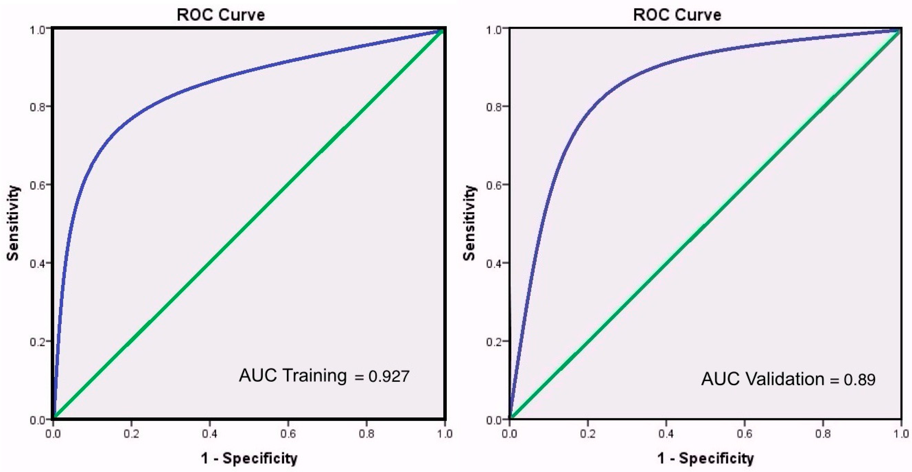
The AUC, as a measure of model performance, presents the trade-off between true and false positive proportions. Here, the AUC represents accuracy without sensitivity to changes in class distribution. The resulting AUC for the 0.5 cut-off value is 0.927 for the training set and 0.89 for the validation set, hence, the 0.5 cut-off value is the selected threshold for the event and non-event decision. Figure 4 below shows the AUC curves for the training and the validation datasets.

Equation (5) above is then incorporated in a Python subroutine that calculates the SLI for each pixel point, 900,000 points to be precise. For each pixel, the algorithm incrementally tries values for SLI from 0 up to the value that causes Equation (4) to provide an output equal to 1, or better said, makes the “probability” of the event become equal to 1. Then, this value is the representative of the minimum amount of water by means of antecedent soil moisture and rainfall value for that pixel.

3.2. Shallow Landslide Index—SMAP/GPM

Based on the short period of time in which the satellites have been in operation, seasonal trends are not identified as of the time of this work. Nonetheless, SMAP and GPM are expected to be functional in almost “real-time” seasonal averaging becomes unnecessary as antecedent root-soil moisture and rainfall can be can be obtained for analysis as soon as seven days prior to date. It is important to have in mind that this work uses not just soil moisture, but root-soil moisture, which encompass the volumetric soil moisture for a 1 m-soil column. As of the writing of this work, this SMAP product has a mean latency of seven days [34].

Three different time intervals are tested: 10-day, 7-day, and 3-day in logistic regression using SPSS software [35]. The significance relationship between the dependent variable and combination of independent variables is expressed on the statistical significance of the model chi-square as seen in

Table 4. Chi-Square.

Model	Chi-Square	Df.	Sig.
10-day	155.484	4	0.000
7-day	156.208	4	0.000
3-day	156.552	4	0.000

.

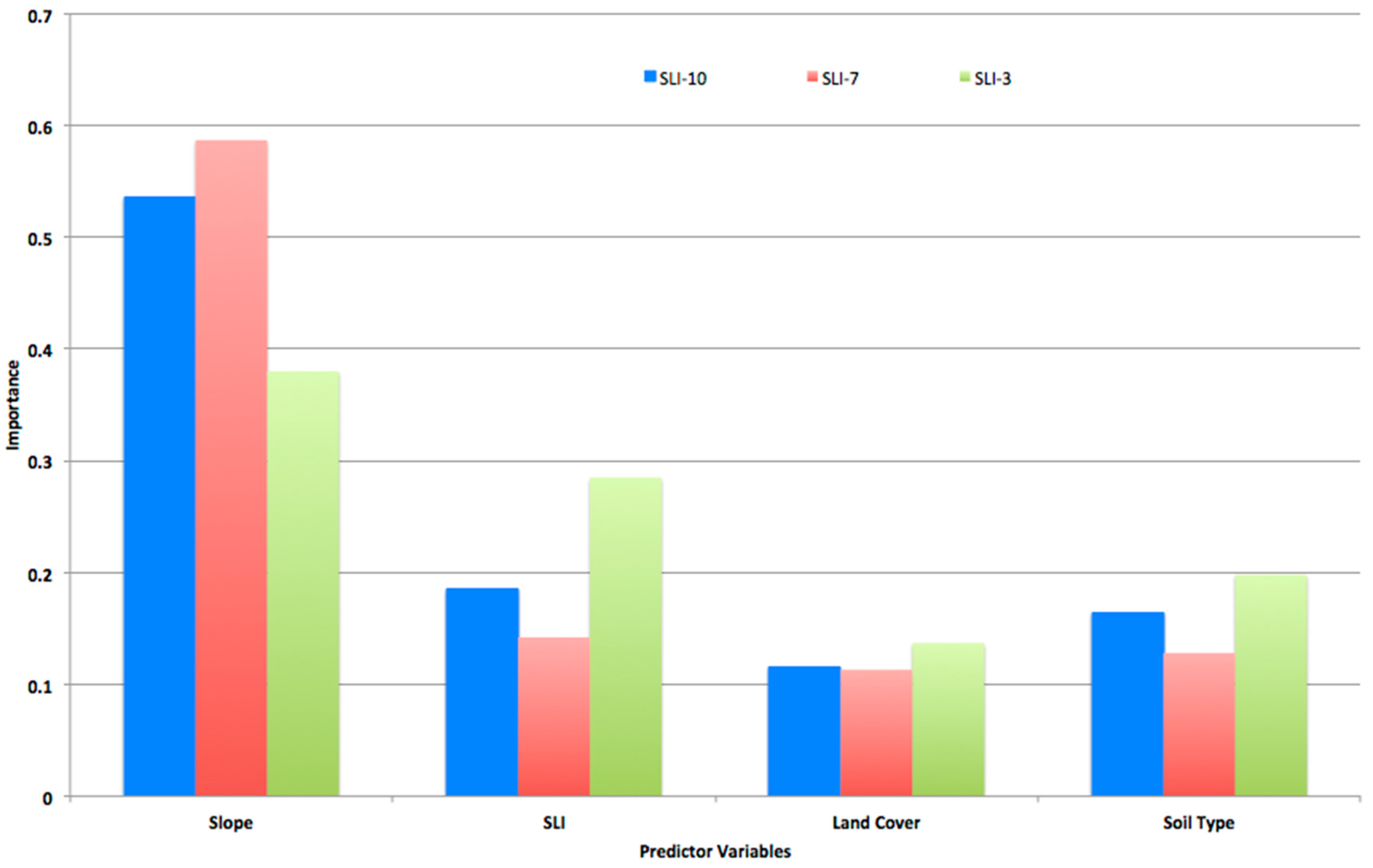
As the significance of all models is <0.001, less than or equal to the level of significance of 0.05, all variables are deemed significant in all models. The null hypothesis that there is no difference between the model with only a constant and the model with independent variables is rejected. Therefore, the existence of a relationship between the independent variables and the dependent variable is supported. In addition, the predictor ranking or variable importance, shown in Figure 5, is also significant for understanding the influence of each variable on the model.

The resulting variable relevance reassures the known conceptual basis of shallow landslides induced by rainfall. Mechanisms that include soil profiles, pore pressures, seepage forces, and soil topography are involved in these results as slope, antecedent soil moisture, and rainfall rank amongst the most significant variables in the model. Soil type and its properties are also involved in the development of shallow landslides and come third in importance in the model. It is the soil’s properties such as its composition that relate to the amount of soil moisture and cohesion among particles that influence landslides. Specifically, the pore water pressures have tremendous effects on slope stability that triggers shallow landslides or slope failures particularly in unstable soils subject to heavy rainfall. Land cover characteristics such as tree roots for stabilization and other hydrological and mechanical influences are also related to landslides, the model uses this variable in almost equal importance to soil type.

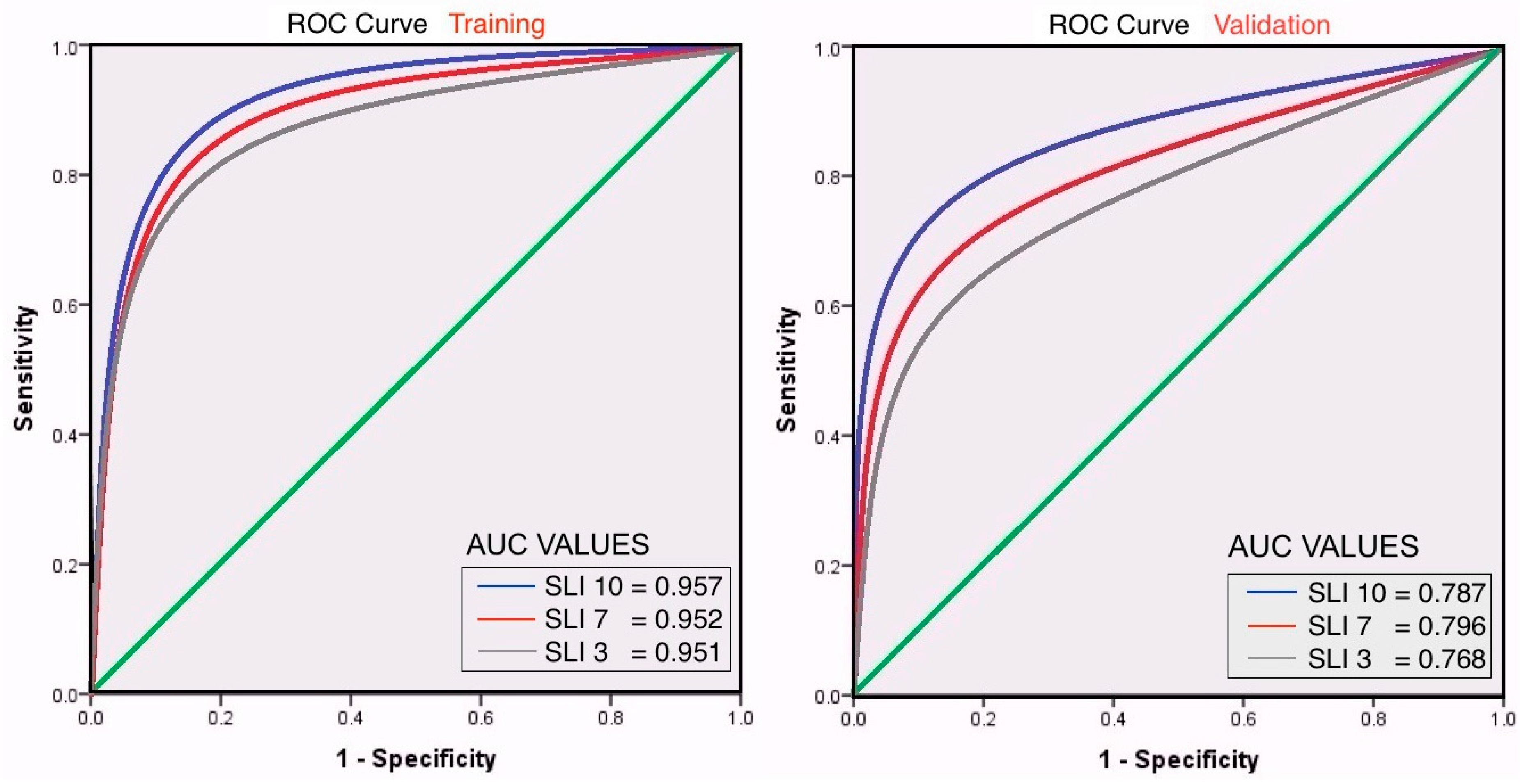
The area under the curve (AUC) as a measure of model performance represents accuracy without sensitivity to changes in class distribution. The resulting AUC for the 0.2 cut-off value is the selected threshold for the event and non-event decision as shown in Figure 6.

Although there is no close analogous statistic in logistic regression to the coefficient of determination R², the Pseudo R² or Nagelkerke R² (that ranges from 0 to 1) for each model describes the goodness of fit for each logistic model, in this case, all validation models are close to 1, therefore indicating a strong relationship (78.7%, 79.6%, and 76.8% respectively) between the predictors and the predicted value.

The resulting equations for the models are:

Z_10-day = ((2.4 × Slope) − (1.425 × Soil Type) + (5.136 × Land Cover) + (4.414 × SLI) − 46.6)

(6)

Z_7-day = ((2.6 × Slope) − (1.657 × Soil Type) + (5.609 × Land Cover) + (5.051 × SLI) − 50.2)

(7)

Z_3-day = ((3.1 × Slope) − (2.452 × Soil Type) + (6.793 × Land Cover) + (6.793 × SLI) − 56.4)

(8)

Each equation is then incorporated in a python subroutine that calculates the SLI for each one of the 900,000 pixels.

3.3. SLI Application

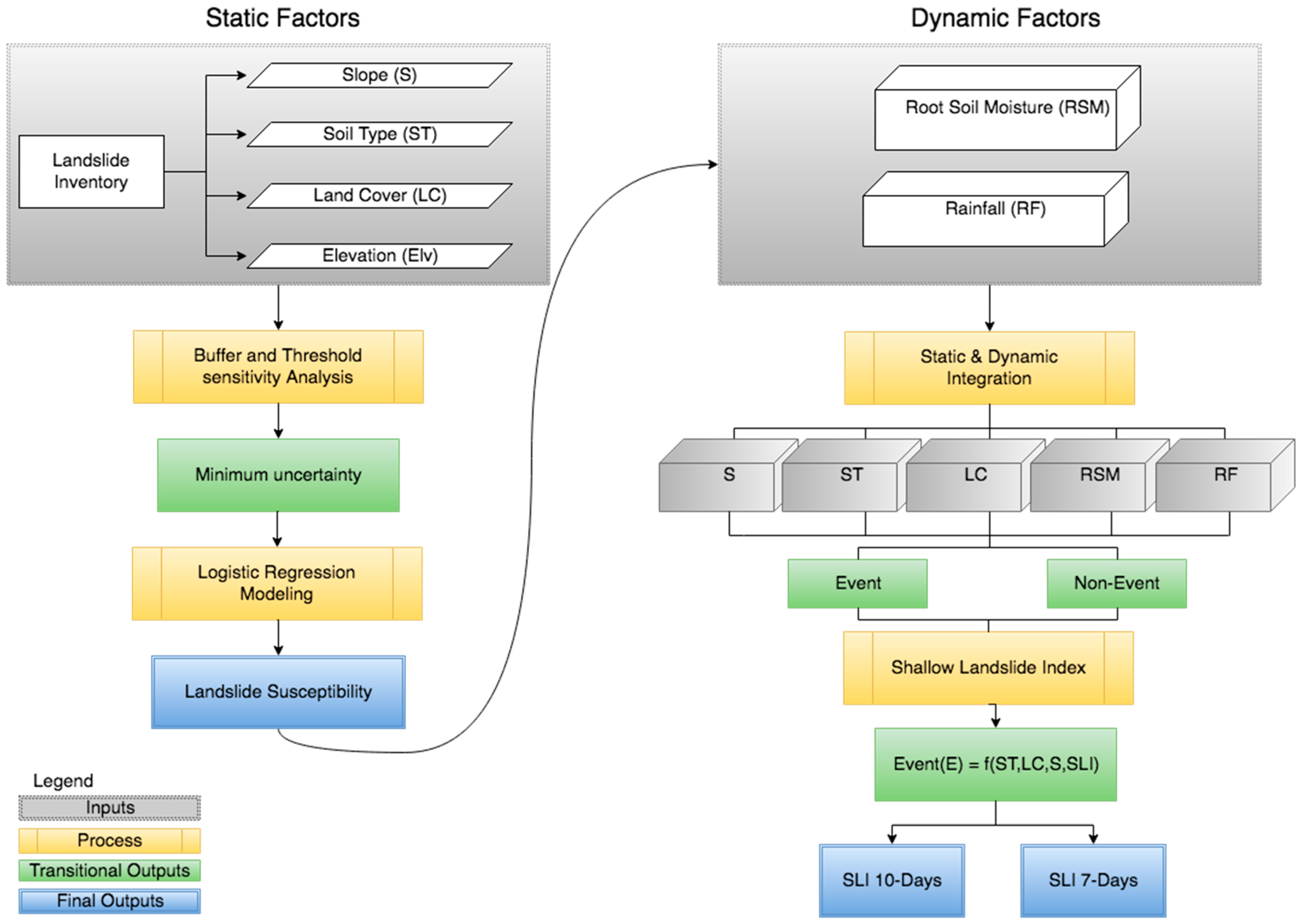
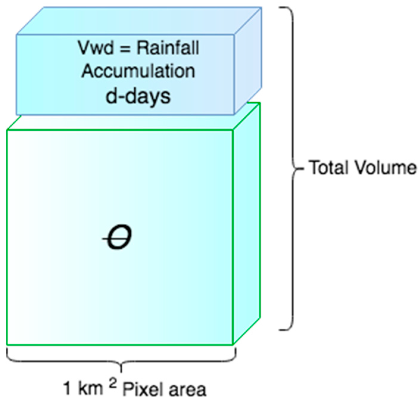
The SLI is built to include the effect of the initial moisture content of the soil and the rainfall depth that is accumulated in a certain period d (days). This period is assumed as the number of days after which the effect of accumulated rainfall will trigger the shallow landslide taking into consideration the initial moisture. Ideally, as a dynamic system, the model will automatically retrieve direct information from SMAP to account for current soil moisture conditions and rainfall forecasts for up to 10 days can be included to calculate the current SLI.

Figure 7 below shows the applied AMSR-E/TRMM SLI and the applied SMAP/GPM SLI. In both maps, each pixel contains a color index value. This value is the critical SLI that will turn Equation (5) equal to 1, in other words, the minimum value of soil moisture content and rainfall accumulation over a 10-day period that is necessary to trigger a shallow landslide. These maps can sever as a baseline to determine shallow landslide hazards. Once the current daily moisture and the forecasted rainfall depth expected in the next 10 days are available, the system can calculate the expected SLI value. This value, in turn, indicates the possibility of a shallow landslide occurrence if it is equal or greater than the critical SLI value.

4. Discussion

4.1. Comparing AMSR-E/TRMM and SMAP/GPM

Both models, AMSR-E and SMAP, are built with the same static variables defined and prepared as described in Section 2. Soil moisture and rainfall estimates differ on both models as they are retrieved from different satellites. Regretfully, there is no overlap between AMRS-E and SMAP, AMSR-E was discontinued in October 2011 and SMAP was launched in January 2015. Even though TMPA information is still being produced, TRMM stopped functioning on April 2015 and GPM took over in 2015; the non-bias comparison is truncated, as sample sizes of each instrument are very different. In this study, for example, seven years of AMSR-E and TRMM data are used versus only nine months of SMAP and GPM information.

Nevertheless, it is important to highlight the instrument’s characteristics to form an understanding of relative performance to each other. In the case of soil moisture, on the one hand, AMSR-E’s daily root-zone soil moisture product is derived from the C-band retrievals into the 2-Layer Palmer Water Balance Model from the LPRM/(AMSR-E)/AQUA surface soil moisture retrievals using a one-dimensional, 30 member Ensemble Kalman filter (EnKF). This model optimally combines soil moisture information derived from the model forecast and satellite retrieval, it then extrapolates surface soil moisture retrievals into deeper root zone soil moisture predictions. AMSR-E did this at a 0.25-degree spatial resolution.

SMAP on the other hand provides estimates of root zone soil moisture for the first 1 m of the soil column using the ensemble Kalman filter (EnKF) that merges SMAP observations with NASA’s catchment land surface model. This land surface model is based on surface meteorological forcing data which includes precipitation and surface processes such as the vertical transfer between the surface and root zone reservoirs, then the model interpolates and extrapolates the satellite observations in time and space. The model and the products are compared to various in situ observations where the model proves of superior quality [34].

In the case of rainfall, GPM builds on TRMM, expanding on spatial footprint and improving on spatial resolution going from 0.25-degrees to 0.1-degrees resolution. In addition, GPM improves on TRMM with the Dual-frequency Precipitation radar and the multi-channel microwave imager that provided higher sensitivity than TRMM.

Here we present the statistical analysis of both model performances, AMSR-E 10-day and SMAP 10-day.

Table 5. SLI-10 & AMSR-E Descriptive Statistics.

Descriptive Statistics
	N	Min.	Max.	Mean		Std.	Var.	Skewness
	ST	ST	ST	ST	Std. Error	ST	ST	ST	Std. Error
SLI_10_Day	3837	6	13	9.48	0.025	1.54	2.373	0.222	0.04
AMSR-E	3837	1	13	9.08	0.026	1.63	2.656	−0.803	0.04

ST—statistic.

shows the Descriptive statistics for 3837 random pixels that were selected for evaluation.

A t-test that measures the significant difference between the two models is performed as shown in

Table 6. SLI-10 & AMSR-E t-test.

	Mean	Std. Dev.	Std. Error Mean	t.	Df.	Sig. (2-Tailed)
Models	0.39927	1.356	0.0218	18.238	3836	0.000

.

Significant variances between the two models are calculated with the F-test, which simply divides the two variances as shown in Equation (9). F-critical at a 95% significance confidence level is equal to 1.054, as F calculated is greater than F-critical, it is concluded that there is significant variance, making the AMSR-E model significantly different from the SMAP model.

$$F=\frac{2.656}{2.373}=1.12$$

(9)

These findings show that both SLI maps, AMSR-E 10-day and SLI 10-day are significantly different and should not be used interchangeably.

4.2. Challenges and Limitations

It is important to stress the limitations of this work. The landslide record in which this system was built does not provide the time of event information. Therefore, daily averages of antecedent root-soil moisture and rainfall are used. Furthermore, antecedent root-soil moisture itself is a model approximation that was not tested in this study. GPM and SMAP each have their limitations and uncertainties, and consequently, they both have a direct effect in the SLI. Confidence on the information was assumed based on the success of the model described in the literature review.

First and foremost, the accuracy of any learning algorithm is based on the accuracy of the landslide inventory and other datasets used [20,36]. Cullen (2016) demonstrated that buffer and threshold techniques provide a solution for the characterization of static parameters when studying shallow landslides over a vast domain; nevertheless, inventories are prone to heterogeneous reporting and lack information regarding the specific time of the event. In the case of this work, having information regarding the time of event could have a significant impact on the SLI modeling. GPM for example provides rainfall information every 3 h, a landslide inventory that provides a time of the event could prove very useful to improve performance.

Second, given SMAP’s biases and ongoing recalibration with the newly available Modern-Era Retrospective analysis for Research and Applications (MERRA-2) reanalysis, a comparison between the information used to build this system and the recalibrated data could be useful to determine accuracy. It is also important to note that the L4_SM product uncertainties vary dynamically and geographically. Driest areas, for example, are associated with low values of uncertainty given that the deeper layer of soil moisture is mostly constant. High uncertainty values are found in southern China where root-soil moisture is known to be highly variable but SMAP observations cannot be incorporated.

SMAP requires information regarding the L-band brightness temperature climatology in order to determine observation-minus-forecast biases; this climatological information is derived from the Soil Moisture Ocean Salinity (SMOS) mission, which does not provide good quality information in areas where radio-frequency interference (RFI) is high. Furthermore, no SMAP brightness temperature is assimilated in mountainous areas such the Rocky and Andes mountains or near large water bodies such as northern Canada, the Amazon, and the Congo rivers. When SMAP data is not available, the L4_SM product provides global soil moisture estimates based on information provided by the model and forcing data [37]. Consequently, caution should be practiced when incorporating these readings into the SLI. It is likely that as SMAP continues to grow and more data becomes available, better certainty can be acquired for further implementation of root-soil moisture in the SLI.

5. Conclusions

This works introduces the Shallow Landslide Index (SLI). The index is intended to be an indicator of antecedent root-soil moisture and rainfall accumulation as a representation of total water volume over a 1 km² pixel area. This index can serve as guidance for the assessment of shallow landslide hazards within susceptible areas in the Continental United States. AMSR-E and TRMM information are used at first as proxies for model development from where findings are as follows:

• The AMSR-E model predicts the highest number of cases correctly at 92.7% accuracy.
• The RMSE between the resulting SLI and the actual events is 0.83 in a scale from 1–13.
• The resulting index map is useful to have an understanding of hazardous areas as precedent soil moisture conditions and rainfall are taken into consideration. Nevertheless, as AMSR-E is no longer functional, current and future guidance is not possible.

AMSR-E and TRMM are used in this work to learn and explore the feasibility of a system that can serve as a guide for antecedent moisture and rainfall triggers of shallow landslides. Nevertheless, as AMSR-E and TRMM stopped working on October 2011 and April 2015 respectively, a solution that works for the future is presented. New functional satellites, SMAP and GPM, are used to retrieve daily-modeled root-soil moisture and rainfall respectively. The SLI is modeled for three different time intervals—10-day, 7-day, and 3-day—and results are as follows:

• Slope is the variable with most influence over the model followed by soil moisture content and rainfall in the form of SLI, soil type, and land cover are subsequently in importance in the three models.
• The pseudo R², the Nagelkerke R² fit for a logistic regression for each model—10-day, 7-day, and 3-day—indicates a strong relationship (78.7%, 79.6%, and 76.8% respectively) between the predictors and the prediction.
• The optimal cut-off value for these logistic regression models as indicated by the AUC is 0.2.
• The RMSE is used to understand the difference between the events and the predicted SLI value for the three models, as the RMSE is scale dependent, RMSE = 1.08, 0.84, 0.97 are considered a low error in the SLI scale of 1–13.
• Comparing AMSR-E’s performance to SMAP’s is not possible even though both models are built with the same predefined static variables. There is no overlap between AMRS-E and SMAP. In addition, the sample sizes of each instrument are very different, seven years of AMSR-E and TRMM versus nine months of SMAP and GPM. Nevertheless, the t-test of significant difference in means and the f-test for significant variance result in significant differences.

The SLI index is intended to present stakeholders with the capability to foresee volumetric water conditions for susceptible locations 10 and 7 days in advance, facilitating the decision-making progress to determine shallow landslide hazard, vulnerability, and risk. Nevertheless, several challenges should be resolved to “fine-tune” the model. These encompass the introduction of a “time of event” parameter into shallow landslide inventories; re-evaluation of SMAP root-soil moisture observations after temperature brightness is re-introduced into the L4_SM model, and the inclusion of other physical parameters should be investigated given the optimal computer power. Future work will include the testing against deterministic infiltration methods for specific events in order to determine how SLI capabilities could be improved, the implementation of the automated system, and the development of SLI for other areas where in situ or deterministic methods are not viable.

References

1. Hong, Y.H.Y.; Adler, R.F.; Huffman, G. An experimental global prediction system for rainfall-triggered landslides using satellite remote sensing and geospatial datasets. IEEE Trans. Geosci. Remote Sens. 2007, 45, 1671–1680. [Google Scholar] [CrossRef]
2. Kirschbaum, D.B.; Adler, R.; Hong, Y.; Hill, S.; Lerner-Lam, A. A global landslide catalog for hazard applications: Method, results, and limitations. Nat. Hazards 2009, 52, 561–575. [Google Scholar] [CrossRef]
3. Cullen, C.; Kashuk, S.; Al-Suhili, R.; Khanbilvardi, R. A multistage technique to minimize overestimations of slope susceptibility at large spatial scales. J. Remote Sens. GIS 2016, 5, 159. [Google Scholar]
4. Aristizábal, E.; Velez, J.; Martínez, C.; Jaboyedoff, M. SHIA_Landslide: A distributed conceptual and physically based model to forecast the temporal and spatial occurrence of shallow landslides triggered by rainfall in tropical and mountainous basins. Landslides 2016, 13, 497–517. [Google Scholar] [CrossRef]
5. Oku, Y.; Nakakita, E. Future change of the potential landslide disasters as evaluated from precipitation data simulated by MRI-AGCM3.1. Hydrol. Process. 2013, 27, 3332–3340. [Google Scholar] [CrossRef]
6. Barbi, F.; da Costa Ferreira, L. Risks and political responses to climate change in Brazilian coastal cities. J. Risk Res. 2013, 17, 485–503. [Google Scholar] [CrossRef]
7. Chae, B.-G.; Kim, M.-I. Suggestion of a method for landslide early warning using the change in the volumetric water content gradient due to rainfall infiltration. Environ. Earth Sci. 2011, 66, 1973–1986. [Google Scholar] [CrossRef]
8. Prokešová, R.; Medveďová, A.; Tábořík, P.; Snopková, Z. Towards hydrological triggering mechanisms of large deep-seated landslides. Landslides 2012, 10, 239–254. [Google Scholar] [CrossRef]
9. Lehmann, P.; Gambazzi, F.; Suski, B.; Baron, L.; Askarinejad, A.; Springman, S.M.; Holliger, K.; Or, D. Evolution of soil wetting patterns preceding a hydrologically induced landslide inferred from electrical resistivity survey and point measurements of volumetric water content and pore water pressure. Water Resour. Res. 2013, 49, 7992–8004. [Google Scholar] [CrossRef]
10. Crosta, G.B.; Frattini, P. Distributed modelling of shallow landslides triggered by intense rainfall. Nat. Hazards Earth Syst. Sci. 2003, 3, 81–93. [Google Scholar] [CrossRef]
11. Collins, B.D.; Znidarcic, D. Stability Analyses of Rainfall Induced Landslides. J. Geotech. Geoenviron. Eng. 2004, 130, 362–372. [Google Scholar] [CrossRef]
12. Segoni, S.; Rosi, A.; Rossi, G.; Catani, F.; Casagli, N. Analysing the relationship between rainfalls and landslides to define a mosaic of triggering thresholds for regional-scale warning systems. Nat. Hazards Earth Syst. Sci. 2014, 14, 2637–2648. [Google Scholar] [CrossRef]
13. Segoni, S.; Rossi, G.; Rosi, A.; Catani, F. Landslides triggered by rainfall: A semi-automated procedure to define consistent intensity–duration thresholds. Comput. Geosci. 2014, 63, 123–131. [Google Scholar] [CrossRef]
14. Floris, M.; Bozzano, F. Evaluation of landslide reactivation: A modified rainfall threshold model based on historical records of rainfall and landslides. Geomorphology 2008, 94, 40–57. [Google Scholar] [CrossRef]
15. Brunetti, M.T.; Peruccacci, S.; Rossi, M.; Luciani, S.; Valigi, D.; Guzzetti, F. Rainfall thresholds for the possible occurrence of landslides in Italy. Nat. Hazards Earth Syst. Sci. 2010, 10, 447–458. [Google Scholar] [CrossRef]
16. Giannecchini, R.; Galanti, Y.; D’Amato Avanzi, G. Critical rainfall thresholds for triggering shallow landslides in the Serchio River Valley (Tuscany, Italy). Nat. Hazards Earth Syst. Sci. 2012, 12, 829–842. [Google Scholar] [CrossRef] [Green Version]
17. Papa, M.N.; Medina, V.; Ciervo, F.; Bateman, A. Derivation of critical rainfall thresholds for shallow landslides as a tool for debris flow early warning systems. Hydrol. Earth Syst. Sci. 2013, 17, 4095–4107. [Google Scholar] [CrossRef]
18. Kirschbaum, D.; Stanley, T.; Yatheendradas, S. Modeling landslide susceptibility over large regions with fuzzy overlay. Landslides 2016, 13, 485–496. [Google Scholar] [CrossRef]
19. Baum, R.L.; Godt, J.W. Early warning of rainfall-induced shallow landslides and debris flows in the USA. Landslides 2009, 7, 259–272. [Google Scholar] [CrossRef]
20. Kirschbaum, D.; Adler, R.; Hong, Y. Advances in landslide nowcasting: Evaluation of a global and regional modeling approach. Environ. Earth Sci. 2012, 66, 1683–1696. [Google Scholar] [CrossRef]
21. Glade, T.; Crozier, M.; Smith, P. Applying probability determination to refine landslide-triggering rainfall thresholds using an empirical “Antecedent Daily Rainfall Model”. Pure Appl. Geophys. 2000, 157, 1059–1079. [Google Scholar] [CrossRef]
22. Liao, Z.; Hong, Y.; Wang, J.; Fukuoka, H.; Sassa, K.; Karnawati, D.; Fathani, F. Prototyping an experimental early warning system for rainfall-induced landslides in Indonesia using satellite remote sensing and geospatial datasets. Landslides 2010, 7, 317–324. [Google Scholar] [CrossRef]
23. Brocca, L.; Ponziani, F.; Moramarco, T.; Melone, F.; Berni, N.; Wagner, W. Improving Landslide Forecasting Using ASCAT-Derived Soil Moisture Data: A Case Study of the Torgiovannetto Landslide in Central Italy. Remote Sens. 2012, 4, 1232–1244. [Google Scholar] [CrossRef]
24. Chen, H.X.; Zhang, L.M. A physically-based distributed cell model for predicting regional rainfall-induced shallow slope failures. Eng. Geol. 2014, 176, 79–92. [Google Scholar] [CrossRef]
25. Aristizábal, E.; García, E.; Martínez, C. Susceptibility assessment of shallow landslides triggered by rainfall in tropical basins and mountainous terrains. Nat. Hazards 2015, 78, 621–634. [Google Scholar] [CrossRef]
26. Godt, J.W.; Baum, R.L.; Chleborad, A.F. Rainfall characteristics for shallow landsliding in Seattle, Washington, USA. Earth Surf. Process. Landf. 2006, 31, 97–110. [Google Scholar] [CrossRef]
27. Van Westen, C.J.; Castellanos, E.; Kuriakose, S.L. Spatial data for landslide susceptibility, hazard, and vulnerability assessment: An overview. Eng. Geol. 2008, 102, 112–131. [Google Scholar] [CrossRef]
28. Land, G.; Share, C.; Latham, J.; Cumani, R.; Rosati, I.; Bloise, M. Global Land Cover SHARE. Available online: http://www.glcn.org/downs/prj/glcshare/GLC_SHARE_beta_v1.0_2014.pdf (accessed on 18 October 2016).
29. Goddard Earth Sciences Data and Information Services Center (GES DISC). TRMM (TMPA) Precipitation L3 1 day 0.25 Degree × 0.25 Degree V7. 2010. Available online: http://disc.sci.gsfc.nasa.gov/datacollection/TRMM_3B42_daily_V7.html (accessed on 18 October 2016). [Google Scholar]
30. GES DISC. TRMM TMPA. 2015. Available online: http://mirador.gsfc.nasa.gov/cgi-bin/mirador/presentNavigation.pl?tree=project (accessed on 18 October 2016). [Google Scholar]
31. Ray, R.L.; Jacobs, J.M.; Ballestero, T.P. Regional landslide susceptibility: Spatiotemporal variations under dynamic soil moisture conditions. Nat. Hazards 2011, 59, 1317–1337. [Google Scholar] [CrossRef]
32. Guns, M.; Vanacker, V. Logistic regression applied to natural hazards: Rare event logistic regression with replications. Nat. Hazards Earth Syst. Sci. 2012, 12, 1937–1947. [Google Scholar] [CrossRef]
33. Food and Agriculture Organization of the United Nations (FAO); Applied International Institute for Systems Analysis (IIASA); ISRIC-World Soil Information; Institute of Soil Science—Chinese Academy of Sciences (ISSCAS); Joint Research Centre of the European Commission (JRC). Harmonized World Soil Database; FAO: Rome, Italy; IIASA: Laxenburg, Austria, 2012. [Google Scholar]
34. Entekhabi, D.; Yueh, S.; O’Neill, P.E.; Kellogg, K.H. SMAP Handbook JPL 400-1567. 2014. Available online: https//smap.jpl.nasa.gov/files/smap2/SMAP_Handbook_FINAL_1_JULY_2014_Web.pdf (accessed on 18 October 2016). [Google Scholar]
35. International Business Machines Corporation (IBM). SPSS; IBM: Armonk, NY, USA, 2013. [Google Scholar]
36. Longoni, L.; Papini, M.; Brambilla, D.; Arosio, D.; Zanzi, L. The role of the spatial scale and data accuracy on deep-seated gravitational slope deformation modeling: The Ronco landslide, Italy. Geomorphology 2016, 253, 74–82. [Google Scholar] [CrossRef]
37. Kimball, J.S.; Jones, L.A.; Glassy, J.; Stavros, E.N.; Madani, N.; Reichle, R.H.; Jackson, N.T.; Colliander, A. Soil Moisture Active Passive Mission L4_C Data Product Assessment (Version 2 Validated Release). 2016. Available online: https://gmao.gsfc.nasa.gov/pubs/docs/Kimball852.pdf (accessed on 18 October 2016). [Google Scholar]
Figure 1. Shallow Landslide Index (SLI) Workflow. (Left) static factors and methods used to establish susceptibility; (Right) Dynamic and static factors integration to determine what combination results in a shallow landslide event. Such combination is expressed in the form of an index calculated for 10 or 7 days of root-soil moisture and rainfall conditions.
Remotesensing 08 00866 g001
Figure 2. Antecedent Soil moisture θ and accumulated rainfall depth in d-days over the pixel area Vwd as the total volume of water content of the Shallow Landslide Index (SLI).
Remotesensing 08 00866 g002
Figure 3. The Shallow Landslide Index (SLI)—for each pixel that contains information about static factors and their corresponding initial soil moisture, the algorithm incrementally tries rainfall values (starting at 0) until it finds the value that makes the logistic regression equation equal to 1.
Remotesensing 08 00866 g003
Figure 4. AUC 0.5 cut-off value AMSR-E/TRMM.
Remotesensing 08 00866 g004
Figure 5. Normalized importance analysis of each variable in the three models indicating the percentage effect of each variable on the dependent variable.
Remotesensing 08 00866 g005
Figure 6. ROC Curve SMAP/GPM models showing the resulting AUC values for all three different time periods tested, SLI 10, 7, and 3 days respectively.
Remotesensing 08 00866 g006
Figure 7. (Top) SLI for 10 days calculated with AMSR-E/TRMM information; (Bottom) SLI for 10 days calculated with SMAP/GPM information. The color bar represents the index number associated to the minimum amount of moisture and rainfall depth accumulation necessary to trigger a shallow landslide at each location. Any new calculated values that are equal or greater to the SLI shall be considered for further investigation, as it is likely that a shallow landslide event could happen.
Remotesensing 08 00866 g007