
Optical Backscattering Measured by Airborne Lidar and Underwater Glider


1
Earth System Research Laboratory, National Oceanic and Atmospheric Administration, 325 Broadway, Boulder, CO 80305, USA
2
Cooperative Institute for Research in Environmental Sciences (CIRES), University of Colorado and National Oceanic and Atmospheric Administration, 325 Broadway, Boulder, CO 80305, USA
3
College of Marine Science, University of South Florida, 140 7th Avenue South, Saint Petersburg, FL 33701, USA
4
MOTE Marine Laboratory & Aquarium, 1600 Ken Thompson Parkway, Sarasota, FL 34236, USA
*
Author to whom correspondence should be addressed.
Remote Sens. 2017, 9(4), 379; https://0-doi-org.brum.beds.ac.uk/10.3390/rs9040379
Submission received: 13 December 2016
/
Revised: 5 April 2017
/
Accepted: 13 April 2017
/
Published: 18 April 2017
Abstract
:The optical backscattering from particles in the ocean is an important quantity that has been measured by remote sensing techniques and in situ instruments. In this paper, we compare estimates of this quantity from airborne lidar with those from an in situ instrument on an underwater glider. Both of these technologies allow much denser sampling of backscatter profiles than traditional ship surveys. We found a moderate correlation (R = 0.28, p < 10−5), with differences that are partially explained by spatial and temporal sampling mismatches, variability in particle composition, and lidar retrieval errors. The data suggest that there are two different regimes with different scattering properties. For backscattering coefficients below about 0.001 m−1, the lidar values were generally greater than the glider values. For larger values, the lidar was generally lower than the glider. Overall, the results are promising and suggest that airborne lidar and gliders provide comparable and complementary information on optical particulate backscattering.
1. Introduction
The spectral characteristics of remote sensing reflectance (Rrs) measured from space have provided a global view of the upper ocean. Remote sensing reflectance is a function of both the apparent and inherent optical properties of water (AOPs and IOPs), the latter of which includes the particulate backscattering coefficient (bbp), the backscattering coefficient of seawater (bbw), and several absorption terms [1,2,3]. Therefore, accurate measurements of bbp are necessary to better understand remote sensing measurements. The use of bbp in expressions for remote sensing reflectance is an approximation, since any ocean color measurement from space is made at a single scattering angle that depends on the solar zenith angle. The approximation is justified by calculations showing an error <10% for a “wide range of scattering phase functions” for solar zenith angles >20° [3]. In more targeted studies, bbp has been related to the total particulate material [4,5], particulate organic carbon [6,7], and the carbon content of phytoplankton [8,9,10].
In situ measurement of bbp is facilitated by the fact that, because the variability in the shape of the particulate volume scattering function at scattering angles >90° is relatively low [11,12,13,14,15,16,17], a relationship between the particulate backscattering coefficient and volume scattering functions that can be expressed as [12,13,14,15,16,17]
where βp(θ) is the particulate volume scattering function at scattering angle θ and χ is a conversion factor defined by this equation. Direct measurement of backscattering at all angles >90° is difficult, but this relationship allows us to estimate bbp from measurement of βp at a single angle, denoted by θ0, [18] with an error around 10% [19]. This can be improved to about 3% using measurements at two scattering angles [20] and to under 1% with a geometry that provides the integrated scattering with a diffuse cavity [19].
Both field [12,13,14,15,17] and laboratory [13,16,21] studies have shown that the variability in χ is minimum at a scattering angle near 120°. Most studies report χ(120°) = 1.10–1.13 with a variability of a few % [12,13,14,15,16,17]. There is less agreement about the behavior of χ at larger scattering angles. Some studies reported lower values for χ(170°) [12,13,16], but most do not [13,15,16,17]. The most recent laboratory measurements, made out to 175°, are significantly lower, reporting χ(175°) < 0.01 for several phytoplankton species and χ(175°) = 0.2 for Arizona road dust [21]. In all cases, the variability is higher at larger scattering angles, which is partially a reflection of difficulties in scattering measurements near 180°.
Compact instruments that measure optical scattering at a single angle with source-receiver separations of a few cm can be deployed on underwater gliders. Gliders are small, autonomous underwater vehicles that manipulate their buoyancy to continuously profile the water column [22] while “gliding” horizontally, collecting thousands of measurements during deployments typically ranging between a few days and a few months. Because of their unique propulsion mechanism, gliders allow energy and cost-efficient measurements on spatial and temporal scales that are difficult to make by other means [23]. Gliders outfitted with fluorometers are routinely used for monitoring the phytoplankton community structure of the West Florida Shelf [24,25,26,27], where they have been particularly useful in describing the 3-dimensional structure of blooms of Karenia brevis, the Florida red-tide organism.
Profiles of optical scattering have been made by airborne lidar [28]. This technique has been particularly effective in measuring enhanced scattering layers in the ocean [29,30] and dynamical processes such as internal waves [31,32]. A direct comparison of airborne lidar estimates of bbp with ship based measurements produced a root-mean square difference of 9.4 × 10⁻⁴ m−1 over a range of values from 5 × 10⁻⁴ m−1 to 9 × 10⁻³ m−1 [33]. This agreement was obtained using χ(180°) = 0.5.
In this work, we describe results from a field campaign in which airborne lidar measurements were obtained simultaneous with glider measurements along a routine harmful algae bloom monitoring transect on the West Florida Shelf. The primary objective of this paper is to compare estimates of bbp from airborne lidar with those from an in situ scatterometer on a glider to determine if these measurements are consistent with one another and can be quantitatively compared to produce a complementary data set.
2. Materials and Methods
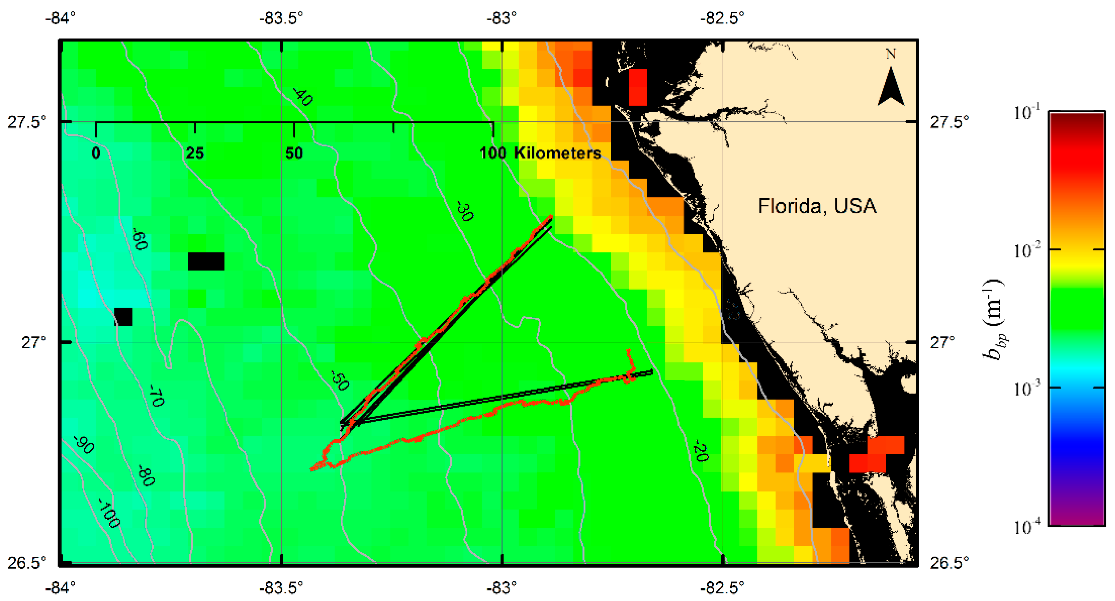
The study area (Figure 1) comprised two transect lines on the West Florida Shelf between Tampa Bay and Charlotte Harbor. In the initial transect design, water depth varied from 20 m at the eastern end of the lines to 50 m at the western end. The northern transect was extended to the southwest past the original waypoint in response to a feature observed in satellite images. The aircraft tracks followed the original design, and this is the reason for the deviation between the glider track and the aircraft tracks in the figure. The background color in the figure is bbp at 531 nm from the Moderate Resolution Imaging Spectroradiometer (MODIS) on the Aqua spacecraft for July 2015. The high values near the coast are probably influenced by the reflection from the sea floor. Over the study region, we see relatively little variation in the surface values as seen from space.
The Slocum G1 glider (Teledyne Webb Research) was deployed at 82.89°W longitude, 27.28°N latitude on 6 July 2015, reached the apex (83.43°W, 26.71°N) on 12 July and turned back towards the coast, and was finally retrieved on 17 July at 82.71°W, 26.98°N. During this period, it made a total of 3372 profiles (up or down) between 2 m below the surface and 2 m above the bottom (Slocum gliders constrain vertical travel using both pressure sensors and altimeters). An ECO-BBFL2 (WET Labs) “puck” in the central payload bay measured scattering of red (650 nm) light at a scattering angle of 124°. The optical backscatter data were processed as follows: first, the sensor calibration was applied to the data to obtain the volume scattering function, β(124°, 650 nm). The contribution from sea water was estimated as
where the reference value βw(90°, 600 nm) = 8.8 × 10⁻⁵ m−1·sr−1 was taken from Morel [34]. This was subtracted from β, leaving the particulate contribution, βp. This was then multiplied by 2πχ with χ = 1.08 (6.8 sr) to get bb(650 nm) [15]. For each of the two transects, these data were averaged into bins of one meter in depth and 0.1° in longitude.
Remote sensing data were collected with the NOAA Oceanographic Lidar on a NOAA Twin Otter aircraft operating at an altitude of 300 m. Both transect lines were flown on 8 July, 10 July, and 13 July. In addition, the northern line was flown on 15 July and on the early morning of 17 July. With slight modifications, the lidar is the same as has been described in previous publications [29,35,36,37]. For this application, the transmitted pulse energy was 100 mJ, pulse length was 12 ns, pulse repetition rate was 30 s−1, wavelength was 532 nm, polarization was linear, and the beam divergence was 17 mrad. Two receiver telescopes were used to provide two lidar channels; one was unpolarized to collect all light regardless of polarization and the other was polarized to collect light cross-polarized with respect to the transmitted light. The receiver telescopes and transmitted beam were aligned to provide complete overlap at the surface. Each telescope had an aperture at the focus of the primary lens to limit the field of view of the receiver to the divergence of the transmitter, an interference filter (1 nm bandwidth) to limit background light, and a photomultiplier tube to convert the collected light into an electrical signal. For each signal, a logarithmic amplifier compressed the dynamic range of the signal and an 8-bit digitizer sampled and recorded the result at 1 GHz. The beam was not scanned, but was instead pointed at a fixed angle of 15° off nadir.
Processing of the unpolarized lidar data involved several steps. For each pulse, strong surface return was identified, and the depth of subsequent samples were obtained using the speed of light in seawater. Profiles were averaged over 25 pulses (about 60 m along the flight track). Next, the logarithm of each of the averaged signal profiles was fit to a quadratic.
where S is the total lidar return, z is depth, and the ci are the fit coefficients. The top of the range for the fit was set at a depth of 5 m so that the surface reflection would not affect the results. The bottom of the range was taken to be the depth at which the signal was 60 dB below the surface return or 0.8 times the water depth, whichever was less for that particular profile. The reason for using a fit was to allow extrapolation to the surface and top smooth out small variations. The quadratic was chosen because it provided the best fit to the profiles overall. The lidar attenuation coefficient is then
Assuming a constant lidar ratio [38], the volume backscatter was then estimated by
where A is a calibration coefficient based on laboratory measurements. The contribution of water to the volume scattering function was estimated by 1.94 × 10⁻⁴ m−1·sr−1 [38] and subtracted from the total to obtain the particulate volume scattering function.
This was converted into an estimate of bbp using a factor of 2π sr (χ = 1). This value for χ is within the range of reported measurements, and the results can easily be scaled to accommodate different values. The ramifications of this choice are considered in Section 4. The resulting data were binned into the same depth and longitude bins as the glider data. A slightly larger depth range was used for the comparison than was used for the fit—2 m to 60 dB or 0.9 times water depth.
To compare glider and lidar data, we calculated the Pearson correlation coefficient of the binned data for each transect of each flight. In scatter plots of these data, we noticed anomalously low values of lidar data, generally near the limit of the depth range. These values were included in the presentation of the binned backscatter, but the deepest bin at each position was removed before calculation of correlations.
The data from the cross-polarized channel were processed in much the same way as those from the unpolarized channel. The primary difference was that the contribution of water to the volume scattering function is zero for the cross-polarized return at a scattering angle of 180°. Also, the calibration coefficient was different for this channel, because the channels are not identical. Since the cross-polarized channel provides an estimate of the cross-polarized component of the volume backscattering coefficient, βX(π), the final result of this process is not bbp but the product of depolarization, d, and bbp, where the depolarization is defined by
The maximum possible value of d is 0.5, when the scattering is completely depolarizing.
3. Results
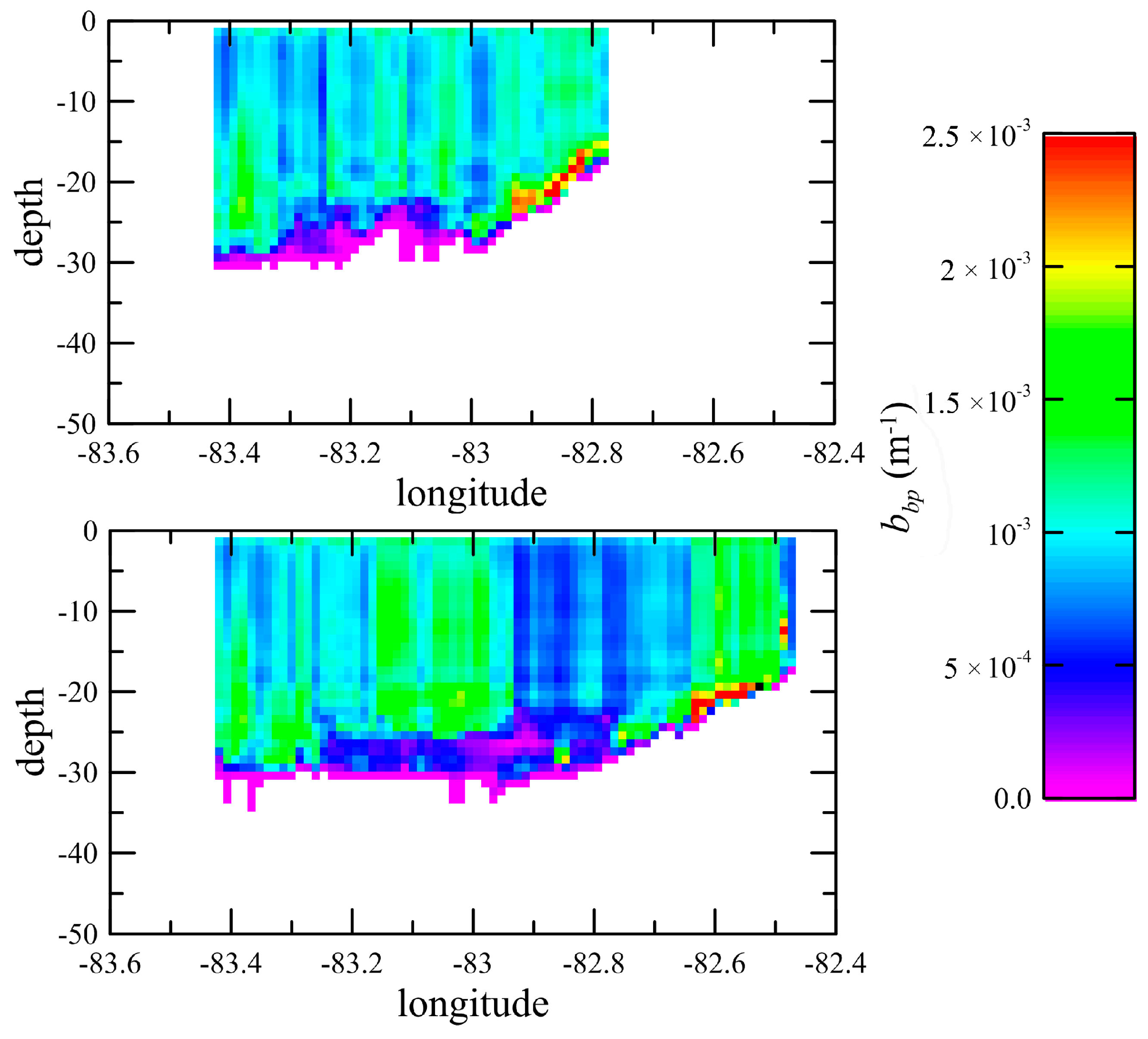
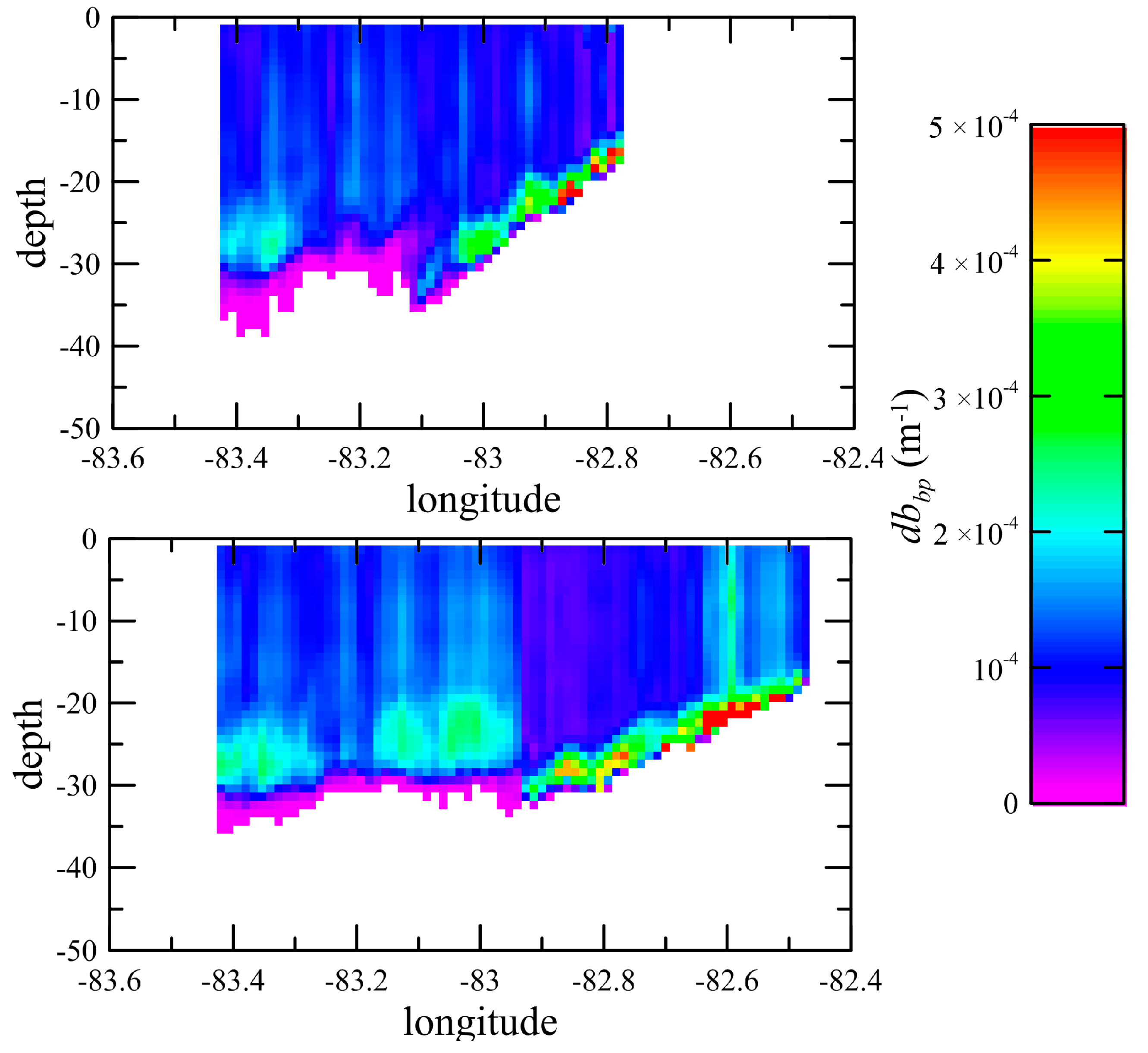
The binned glider data (Figure 2) show enhanced backscatter near the bottom on both transects. Both legs also show enhanced backscatter between 20 and 30 m depths in the western part of each transect. The binned lidar data (Figure 3) show similar features, but there are significant differences. The major features were similar in all flights; the figure shows the average of the first three flights, where we have data from both transects. The major difference is that the lidar signal only penetrates to about 30 m, and the enhancement near the bottom cannot be seen in the western part of the transects where the bottom is deeper than that. The other obvious difference is that the contrast between regions of strong scattering and general background levels is greater in the in situ data than in the lidar data. These data also clearly show the very low values near the bottom of the depth range.
Significant correlations were obtained between the glider and the unpolarized lidar bbp data (Table 1), with an overall average of R = 0.28. Because of the large number of points in each correlation (1100 for the northern transect and 1600 for the longer southern transect), all were highly significant (p < 10−5), except for two flights where the correlation for the cross-polarized return was not significantly correlated with the glider data. The average correlation for the northern transect was slightly greater than for the southern transect (0.32 vs. 0.21), consistent with the better spatial and temporal match between the northern transect flight and glider tracks. The best correlation was observed on the northern transect when the glider was closest to the center of the transect (10 July). The results for the cross-polarized lidar return were similar, with an overall average correlation of R = 0.45 between lidar and glider-measured bbp and higher correlation on the northern transect than on the southern (0.48 vs. 0.38).
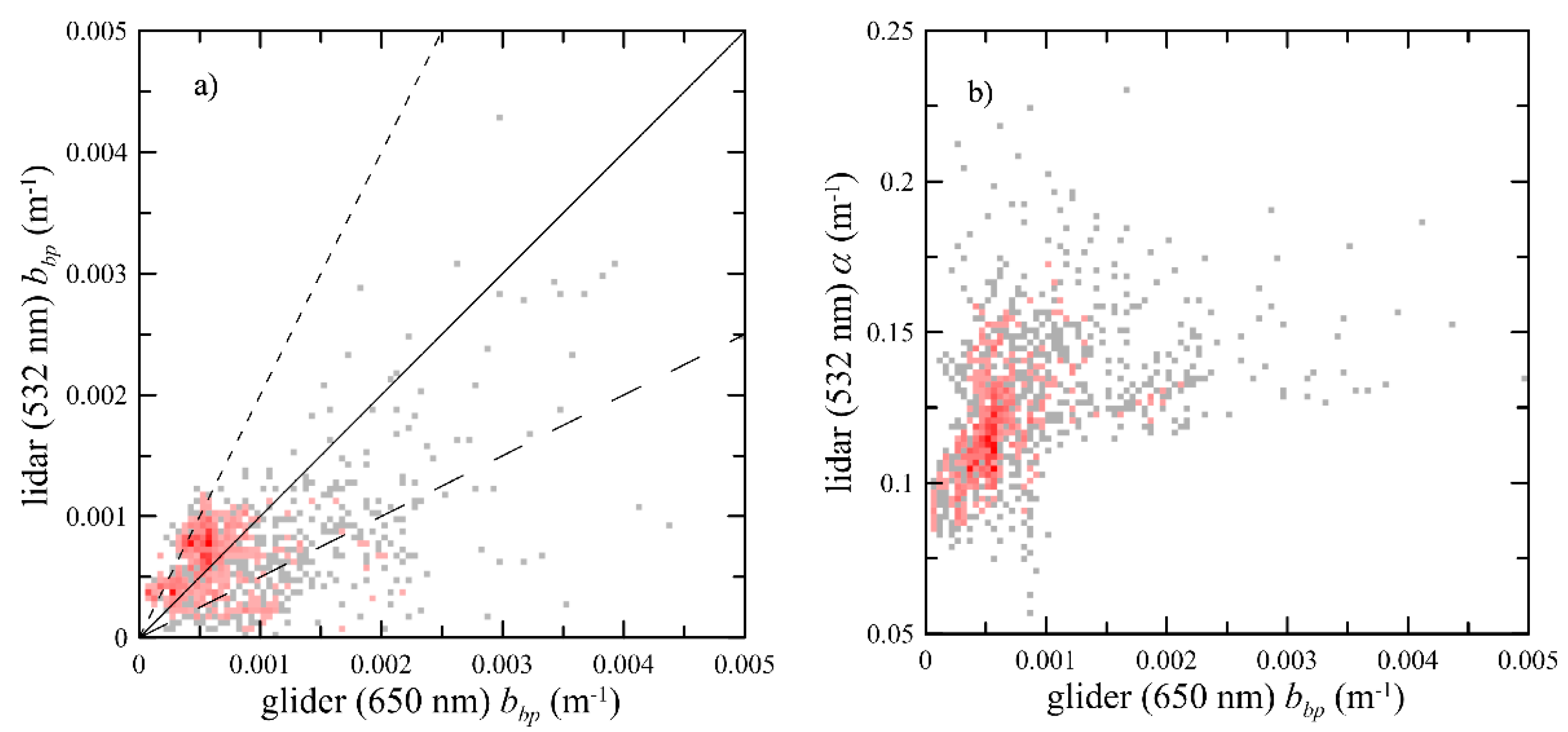
As an example of the scatter in the data, we present the data for the north transect on 10 July (Figure 4). The backscatter values (Figure 4a) are scattered around the 1:1 line, but the figure suggests that there are two different regimes. For values below about 0.001 m−1, the lidar data are generally greater than the glider data. For larger values, the lidar data are generally lower than the glider data. When averaged over all flights, the lidar data were 71% higher than the glider data for the small values, but 30% lower for the large values. There was no difference when the north and south transects were treated separately. The root-mean square (rms) difference between lidar and glider-measured bbp for this flight was 5.4 × 10⁻⁴ m−1. The average over all flights, 8.6 × 10⁻⁴ m−1, was slightly less than previous results [33]. Removing the effects of the difference in mean values, we found the rms difference to be 73% of the average glider value for the low values and 50% for the high values. The short dashed line is the figure shows what the 1:1 line would be, relative to the data, had we used χ(180°) = 0.5. Most of the low values are between these two lines, while most of the high values fall below the 1:1 line obtained with χ(180°) = 1, but above the long dashed lined obtained with χ(180°) = 2. There is also evidence of the two regimes in the lidar attenuation values (Figure 4b), where the attenuation at the higher backscatter values is less than might be expected from an extrapolation of the trend in the lower values.
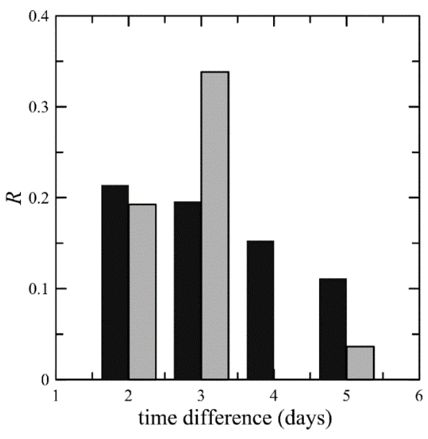
As expected, there was some variability from flight to flight. The correlation between flights is plotted in Figure 5 as a function of the number of days between the flights. For the northern transect, there were three pairs of flights separated by 2 days and two separated by 5 days, and the numbers are averages of these values. The other points represent single pairs of flights. Overall, the correlation at a 2 day separation is similar to the correlation between the lidar and the glider—significant, but not very high. This correlation decreases with increasing delay.
The results for the cross-polarized return, which include the effects of both d and bbp, (Figure 6) show similar patterns to the unpolarized return lidar signal. The contrast between the scattering layers and background levels is greater, however, consistent with previous observations [30,31]. The scattering from pure sea water of 650 nm light at 124° is less than that of 532 nm light at 180° by a factor of 0.29, so the contrast from the scatterometer will be higher than that from the unpolarized lidar return. There is no cross-polarized lidar return from pure sea water, so the contrast is also higher than that from the unpolarized lidar return.
4. Discussion
This work highlights similarities and differences in the measurement of bbp by airborne lidar and glider-based in situ instruments. Both use a measurement of scattering at a single angle to infer bbp. This probably works better for the in situ scattering angle near 120°, because there is less variability in the relationship between bbp and scattering at this angle than there is at the lidar scattering angle of 180° [12,13,14,15,16,17]. Both provide much greater sampling density than traditional ship surveys. This is especially true for the airborne lidar, which can cover transects like those in this study in minutes. However, the lidar depth penetration is limited to about 30 m in coastal waters like the west Florida shelf.
The correlation between lidar and glider results was not perfect, and one reason is probably the mismatch in sampling times and volumes. The overall correlation was greater on the northern transect than on the southern one, which is likely a result of a better match on the northern transect. The temporal variability in the distribution of scattering in the water is evident in the correlations between lidar data from different flights. These correlations are lower when there was a five-day temporal separation than when the separation was two or three days.
Another reason for moderate correlations might be that the assumption of a constant value for χ is not valid. It seems likely that the strong scattering near the bottom is primarily a result of suspended sediments with different particle sizes and refractive indices than the algal cells higher in the water column. This would affect the lidar estimates more than the glider estimates. The reason is that the measured variability of χ at 124°, the angle of the glider instrument, is less than that at larger scattering angles. These measurements generally extend only to 170°, but there is no reason to expect that the higher variability does not also extend to the lidar scattering angle of 180°.
There are some remaining issues to be resolved for accurate measurements of bbp by airborne lidar. The biggest issue is probably the development of a robust lidar inversion technique [39]. The technique used in this work assumed that the attenuation was slowly varying with depth. At the greatest depths, the attenuation of the lidar signal was 60 dB. Small errors in estimating this attenuation correspond to large errors in the corrected signal, because the correction is exponential. One possible solution is provided by the High Spectral Resolution Lidar (HSRL) that measures scattering and attenuation independently [33,40].
Another issue is the uncertainty in χ(180°). Typical measurements extent only out to 170°. Some of these report χ(170°) > 1 [15,17], while others report χ(170°) < 1 [12,13,16]. More recent laboratory instruments are even lower than most previous measurements, with χ(175°) < 0.01 for several algal species [21]. There are also uncertainties in the wavelength dependence of this quantity [41,42,43]. For a power-law spectrum with an exponent of unity, the lidar backscattering would be 22% greater than that from glider. A previous lidar study at 532 nm used χ(180°) = 0.5 [33]. Here we used 1.0. This produced bbp from the lidar that was higher than that measured by the glider by 71% for low values and lower by 30% for high values. This would suggest that we have two different populations of scattering particles with χ(180°) = 0.58 and χ(180°) = 1.43, respectively. All of these values are within the uncertainty in χ(180°), and measurements specifically at this angle are required. This will require development of a new instrument, since current approaches to phase function measurements cannot be extended to 180°.
For the cross-polarized channel, the situation is even more difficult. We not only need to know χ(180°), but also d(180°). There is probably even more uncertainty in this parameter, although some measurements of the polarization properties have been made [44,45,46,47]. For spherical particles, d = 0 [48], so this parameter provides some information on the properties of the scatterers, but more work will be required to exploit this fully. Despite this difficulty, the cross-polarized channel provides greater contrast of high scattering regions and generally greater correlations with the glider data.
A related issue is uncertainty in lidar calibration. If the particulate contribution to the signal is much larger than the pure water component, the effect is nearly linear. If the particulate contribution is small, however, small errors in estimates of total volume scattering coefficient can produce large errors in estimates of the particulate component. Our current calibration error is estimated to be more than 10%, and improving this calibration is an ongoing effort. The source of the error seems to be a large temperature difference between calibration laboratory and the actual operating conditions on the aircraft.
One promising future application of the lidar technique is the global measurement of bbp from space. Preliminary investigations have demonstrated that data from an existing aerosol lidar on the Cloud-Aerosol Lidar and Infrared Pathfinder Satellite Observations (CALIPSO) satellite can detect sub-surface oceanic scattering [49,50,51]. This system, designed for atmospheric measurements, does not have sufficient range resolution for detailed profiles of oceanic backscatter, but airborne measurements have demonstrated that a future orbiting lidar designed for both atmospheric and oceanic profiling could provide valuable information.
5. Conclusions
The primary conclusion of this work is that airborne lidar and gliders provide consistent and complementary information on optical particulate backscattering distributions. The observed correlations, although moderate (R = 0.28 for the unpolarized lidar channel and R = 0.45 for the cross-polarized channel), show similar patterns in estimates of bbp despite differences in wavelength, scattering angle, and measurement volume. These measurements are complementary in the spatial-temporal scales that can be measured. The aircraft provides a measurement that is more nearly synoptic, but cannot measure to the depths or with the spatial detail provided by gliders.
At the same time, quantitative estimates of bbp from the lidar are limited by uncertainties in calibration, lidar retrieval, and χ(180°). The resulting error in the absolute estimates is probably not better than 3 dB. Improving understanding of the properties of χ(180°) will likely require development of a new in situ instrument.
Acknowledgments
Glider surveys supported with funding from the Florida Fish & Wildlife Conservation Commission/Fish & Wildlife Research Institute, Agreement No. 12054. Aircraft surveys were supported by the National Oceanic and Atmospheric Administration.
Author Contributions
James H. Churnside and Richard D. Marchbanks collected the airborne data. Chad Lembke and Jordon Beckler collected and processed the glider data. James H. Churnside analyzed the lidar data. James H. Churnside performed the comparison and wrote the paper.
Conflicts of Interest
The authors declare no conflict of interest. The founding sponsors had no role in the design of the study; in the collection, analyses, or interpretation of data; in the writing of the manuscript, and in the decision to publish the results.
References
- Morel, A.; Prieur, L. Analysis of variations in ocean color. Limnol. Oceanogr. 1977, 22, 709–722. [Google Scholar] [CrossRef]
- Gordon, H.R.; Brown, O.B.; Evans, R.H.; Brown, J.W.; Smith, R.C.; Baker, K.S.; Clark, D.K. A semianalytic radiance model of ocean color. J. Geophys. Res. Atmos. 1988, 93, 10909–10924. [Google Scholar] [CrossRef]
- Maritorena, S.; Siegel, D.A.; Peterson, A.R. Optimization of a semianalytical ocean color model for global-scale applications. Appl. Opt. 2002, 41, 2705–2714. [Google Scholar] [CrossRef] [PubMed]
- Boss, E.; Taylor, L.; Gilbert, S.; Gundersen, K.; Hawley, N.; Janzen, C.; Johengen, T.; Purcell, H.; Robertson, C.; Schar, D.W.H.; et al. Comparison of inherent optical properties as a surrogate for particulate matter concentration in coastal waters. Limnol. Oceanogr. Methods 2009, 7, 803–810. [Google Scholar] [CrossRef]
- Reynolds, R.A.; Stramski, D.; Neukermans, G. Optical backscattering by particles in arctic seawater and relationships to particle mass concentration, size distribution, and bulk composition. Limnol. Oceanogr. 2016, 61, 1869–1890. [Google Scholar] [CrossRef]
- Stramski, D.; Reynolds, R.A.; Babin, M.; Kaczmarek, S.; Lewis, M.R.; Röttgers, R.; Sciandra, A.; Stramska, M.; Twardowski, M.S.; Franz, B.A.; et al. Relationships between the surface concentration of particulate organic carbon and optical properties in the eastern South Pacific and eastern Atlantic Oceans. Biogeosciences 2008, 5, 171–201. [Google Scholar] [CrossRef]
- Stramski, D.; Reynolds, R.A.; Kahru, M.; Mitchell, B.G. Estimation of particulate organic carbon in the ocean from satellite remote sensing. Science 1999, 285, 239–242. [Google Scholar] [CrossRef] [PubMed]
- Behrenfeld, M.J.; Boss, E.; Siegel, D.A.; Shea, D.M. Carbon-based ocean productivity and phytoplankton physiology from space. Glob. Biogeochem. Cycles 2005, 19. [Google Scholar] [CrossRef]
- Martinez-Vicente, V.; Dall’Olmo, G.; Tarran, G.; Boss, E.; Sathyendranath, S. Optical backscattering is correlated with phytoplankton carbon across the Atlantic Ocean. Geophys. Res. Lett. 2013, 40, 1154–1158. [Google Scholar] [CrossRef]
- Graff, J.R.; Westberry, T.K.; Milligan, A.J.; Brown, M.B.; Dall’Olmo, G.; Dongen-Vogels, V.V.; Reifel, K.M.; Behrenfeld, M.J. Analytical phytoplankton carbon measurements spanning diverse ecosystems. Deep Sea Res. Part I 2015, 102, 16–25. [Google Scholar] [CrossRef]
- Petzold, T.J. Volume Scattering Functions for Selected Ocean Waters; Scripps Institution of Oceanography: La Jolla, CA, USA, 1972. [Google Scholar]
- Boss, E.; Pegau, W.S. Relationship of light scattering at an angle in the backward direction to the backscattering coefficient. Appl. Opt. 2001, 40, 5503–5507. [Google Scholar] [CrossRef] [PubMed]
- Chami, M.; Marken, E.; Stamnes, J.J.; Khomenko, G.; Korotaev, G. Variability of the relationship between the particulate backscattering coefficient and the volume scattering function measured at fixed angles. J. Geophys. Res. Oceans 2006, 111, C05013. [Google Scholar] [CrossRef]
- Berthon, J.-F.; Shybanov, E.; Lee, M.E.G.; Zibordi, G. Measurements and modeling of the volume scattering function in the coastal northern Adriatic Sea. Appl. Opt. 2007, 46, 5189–5203. [Google Scholar] [CrossRef] [PubMed]
- Sullivan, J.M.; Twardowski, M.S. Angular shape of the oceanic particulate volume scattering function in the backward direction. Appl. Opt. 2009, 48, 6811–6819. [Google Scholar] [CrossRef] [PubMed]
- Whitmire, A.L.; Pegau, W.S.; Karp-Boss, L.; Boss, E.; Cowles, T.J. Spectral backscattering properties of marine phytoplankton cultures. Opt. Express 2010, 18, 15073–15093. [Google Scholar] [CrossRef] [PubMed]
- Zhang, X.; Boss, E.; Gray, D.J. Significance of scattering by oceanic particles at angles around 120 degree. Opt. Express 2014, 22, 31329–31336. [Google Scholar] [CrossRef] [PubMed]
- Sullivan, J.; Twardowski, M.; Ronald, J.; Zaneveld, V.; Moore, C. Measuring optical backscattering in water. In Light Scattering Reviews 7; Springer: Berlin/Heidelberg, Germany, 2013; pp. 189–224. [Google Scholar]
- Haubrich, D.; Musser, J.; Fry, E.S. Instrumentation to measure the backscattering coefficient bb for arbitrary phase functions. Appl. Opt. 2011, 50, 4134–4147. [Google Scholar] [CrossRef] [PubMed]
- Tan, H.; Oishi, T.; Tanaka, A.; Doerffer, R. Accurate estimation of the backscattering coefficient by light scattering at two backward angles. Appl. Opt. 2015, 54, 7718–7733. [Google Scholar] [CrossRef] [PubMed]
- Harmel, T.; Hieronymi, M.; Slade, W.; Röttgers, R.; Roullier, F.; Chami, M. Laboratory experiments for inter-comparison of three volume scattering meters to measure angular scattering properties of hydrosols. Opt. Express 2016, 24, A234–A256. [Google Scholar] [CrossRef] [PubMed]
- Rudnick, D.L.; Davis, R.E.; Eriksen, C.C.; Frantantoni, D.M.; Perry, M.J. Underwater gliders for ocean research. Mar. Technol. Soc. J. 2004, 38, 48–59. [Google Scholar] [CrossRef]
- Cetinić, I.; Perry, M.J.; D’Asaro, E.; Briggs, N.; Poulton, N.; Sieracki, M.E.; Lee, C.M. A simple optical index shows spatial and temporal heterogeneity in phytoplankton community composition during the 2008 North Atlantic bloom experiment. Biogeosciences 2015, 12, 2179–2194. [Google Scholar] [CrossRef]
- English, D.; Hu, C.; Lembke, C.; Weisberg, R.; Edwards, D.; Lorenzoni, L.; Gonzalez, G.; Muller-Karger, F. Observing the 3-dimensional distribution of bio-optical properties of West Florida Shelf waters using gliders and autonomous platforms. In Proceedings of the OCEANS 2009, MTS/IEEE Biloxi-Marine Technology for Our Future: Global and Local Challenges, Biloxi, MS, USA, 26–29 October 2009; pp. 1–7. [Google Scholar]
- Hu, C.; Barnes, B.B.; Qi, L.; Lembke, C.; English, D. Vertical migration of Karenia brevis in the northeastern Gulf of Mexico observed from glider measurements. Harmful Algae 2016, 58, 59–65. [Google Scholar] [CrossRef] [PubMed]
- Weisberg, R.H.; Zheng, L.; Liu, Y.; Corcoran, A.A.; Lembke, C.; Hu, C.; Lenes, J.M.; Walsh, J.J. Karenia brevis blooms on the West Florida Shelf: A comparative study of the robust 2012 bloom and the nearly null 2013 event. Cont. Shelf Res. 2016, 120, 106–121. [Google Scholar] [CrossRef]
- Zhao, J.; Hu, C.; Lenes, J.M.; Weisberg, R.H.; Lembke, C.; English, D.; Wolny, J.; Zheng, L.; Walsh, J.J.; Kirkpatrick, G. Three-dimensional structure of a Karenia brevis bloom: Observations from gliders, satellites, and field measurements. Harmful Algae 2013, 29, 22–30. [Google Scholar] [CrossRef]
- Churnside, J.H. Review of profiling oceanographic lidar. Opt. Eng. 2014, 53, 051405. [Google Scholar] [CrossRef]
- Churnside, J.H.; Marchbanks, R. Sub-surface plankton layers in the Arctic Ocean. Geophys. Res. Lett. 2015, 42, 4896–4902. [Google Scholar] [CrossRef]
- Churnside, J.H.; Donaghay, P.L. Thin scattering layers observed by airborne lidar. ICES J. Mar. Sci. 2009, 66, 778–789. [Google Scholar] [CrossRef]
- Churnside, J.H.; Ostrovsky, L.A. Lidar observation of a strongly nonlinear internal wave train in the Gulf of Alaska. Int. J. Remote Sens. 2005, 26, 167–177. [Google Scholar] [CrossRef]
- Churnside, J.H.; Marchbanks, R.D.; Lee, J.H.; Shaw, J.A.; Weidemann, A.; Donaghay, P.L. Airborne lidar detection and characterization of internal waves in a shallow fjord. J. Appl. Remote Sens. 2012, 6, 063611. [Google Scholar] [CrossRef]
- Hair, J.; Hostetler, C.; Hu, Y.; Behrenfeld, M.; Butler, C.; Harper, D.; Hare, R.; Berkoff, T.; Cook, A.; Collins, J.; et al. Combined atmospheric and ocean profiling from an airborne high spectral resolution lidar. EPJ Web Conf. 2016, 119, 22001. [Google Scholar] [CrossRef]
- Morel, A. Optical properties of pure water and pure sea water. In Optical Aspects of Oceanography; Jerlov, N.G., Nielsen, E.S., Eds.; Academic Press: San Diego, CA, USA, 1974; Volume 1, pp. 1–24. [Google Scholar]
- Churnside, J.H. Polarization effects on oceanographic lidar. Opt. Express 2008, 16, 1196–1207. [Google Scholar] [CrossRef] [PubMed]
- Churnside, J.H.; Marchbanks, R.D.; Donaghay, P.L.; Sullivan, J.M.; Graham, W.M.; Wells, R.J.D. Hollow aggregations of moon jellyfish (Aurelia spp.). J. Plankton Res. 2016, 38, 122–130. [Google Scholar] [CrossRef]
- Churnside, J.H.; Wells, R.J.D.; Boswell, K.M.; Quinlan, J.A.; Marchbanks, R.D.; McCarty, B.J.; Sutton, T.T. Surveying the distribution and abundance of flyingfishes and other epipelagics in the northern Gulf of Mexico using airborne lidar. Bull. Mar. Sci. 2016, in press. [Google Scholar]
- Churnside, J.H.; Sullivan, J.M.; Twardowski, M.S. Lidar extinction-to-backscatter ratio of the ocean. Opt. Express 2014, 22, 18698–18706. [Google Scholar] [CrossRef] [PubMed]
- Klett, J.D. Stable analytical inversion solution for processing lidar returns. Appl. Opt. 1981, 20, 211–220. [Google Scholar] [CrossRef] [PubMed]
- Hair, J.W.; Hostetler, C.A.; Cook, A.L.; Harper, D.B.; Ferrare, R.A.; Mack, T.L.; Welch, W.; Izquierdo, L.R.; Hovis, F.E. Airborne high spectral resolution lidar for profiling aerosol optical properties. Appl. Opt. 2008, 47, 6734–6752. [Google Scholar] [CrossRef] [PubMed]
- Morel, A. Optical modeling of the upper ocean in relation to its biogenous matter content (Case I waters). J. Geophys. Res. Oceans 1988, 93, 10749–10768. [Google Scholar] [CrossRef]
- Tiwari, S.P.; Shanmugam, P. An optical model for deriving the spectral particulate backscattering coefficients in oceanic waters. Ocean Sci. 2013, 9, 987–1001. [Google Scholar] [CrossRef]
- Dall’Olmo, G.; Boss, E.; Behrenfeld, M.; Westberry, T. Particulate optical scattering coefficients along an Atlantic meridional transect. Opt. Express 2012, 20, 21532–21551. [Google Scholar] [CrossRef] [PubMed]
- Fry, E.S.; Voss, K.J. Measurement of the mueller matrix for phytoplankton1. Limnol. Oceanogr. 1985, 30, 1322–1326. [Google Scholar] [CrossRef]
- Volten, H.; de Haan, J.F.; Hovenier, J.W.; Schreurs, R.; Vassen, W.; Dekker, A.G.; Hoogenboom, H.J.; Charlton, F.; Wouts, R. Laboratory measurements of angular distributions of light scattered by phytoplankton and silt. Limnol. Oceanogr. 1998, 43, 1180–1197. [Google Scholar] [CrossRef]
- Svensen, O.; Stamnes, J.J.; Kildemo, M.; Aas, L.M.S.; Erga, S.R.; Frette, O. Mueller matrix measurements of algae with different shape and size distributions. Appl. Opt. 2011, 50, 5149–5157. [Google Scholar] [CrossRef] [PubMed]
- Zhai, P.-W.; Hu, Y.; Trepte, C.R.; Winker, D.M.; Josset, D.B.; Lucker, P.L.; Kattawar, G.W. Inherent optical properties of the coccolithophore: Emiliania huxleyi. Opt. Express 2013, 21, 17625–17638. [Google Scholar] [CrossRef] [PubMed]
- Van de Hulst, H.C. Light Scattering by Small Particles; Dover: New York, NY, USA, 1981; p. 470. [Google Scholar]
- Lu, X.; Hu, Y.; Trepte, C.; Zeng, S.; Churnside, J.H. Ocean subsurface studies with the CALIPSO spaceborne lidar. J. Geophys. Res. Oceans 2014, 119, 4305–4317. [Google Scholar] [CrossRef]
- Churnside, J.; McCarty, B.; Lu, X. Subsurface ocean signals from an orbiting polarization lidar. Remote Sens. 2013, 5, 3457–3475. [Google Scholar] [CrossRef]
- Behrenfeld, M.J.; Hu, Y.; Hostetler, C.A.; Dall’Olmo, G.; Rodier, S.D.; Hair, J.W.; Trepte, C.R. Space-based lidar measurements of global ocean carbon stocks. Geophys. Res. Lett. 2013, 40, 4355–4360. [Google Scholar] [CrossRef]
Figure 1.
Chart of the study area off the west coast of Florida, USA. Gray lines are depth contours in m. Red line is the glider track. Black lines are the flight track segments used in the analysis. Background is satellite estimate of bbp with values given by the color bar on the right.
Figure 1.
Chart of the study area off the west coast of Florida, USA. Gray lines are depth contours in m. Red line is the glider track. Black lines are the flight track segments used in the analysis. Background is satellite estimate of bbp with values given by the color bar on the right.

Figure 2.
Glider-measured particulate backscattering coefficient bbp as a function of depth and longitude according to the color table at the right. Plot shows the glider data binned into 0.01° latitude by 1 m depth bins for the east to west (top) and return transect (bottom).
Figure 2.
Glider-measured particulate backscattering coefficient bbp as a function of depth and longitude according to the color table at the right. Plot shows the glider data binned into 0.01° latitude by 1 m depth bins for the east to west (top) and return transect (bottom).

Figure 3.
Particulate backscatter coefficient bbp as a function of depth and longitude according to the color table at the right. Top panel is the northern transect and bottom panel is the southern transect. Plot shows the lidar data averaged over the first three flights and binned into 0.01° latitude by 1 m depth bins.

Figure 4.
(a) Scatter plot of binned particulate backscatter coefficient bbp as measured by lidar at 532 nm (unpolarized) as a function of those inferred from the glider data at 650 nm for the north transect. Grey squares denote a single data point within the region covered by the square (5 × 10⁻⁵ m−1 in each dimension). Red squares denote multiple data points from two (lightest) to 20 (darkest shade) of 1228 total. Lidar data are from the 10 July flight. Solid line is the ideal 1:1 relationship for χ(180°) = 1. Short dashes show the 1:1 line, relative to the data, for χ(180°) = 0.5, and long dashes for χ(180°) = 2.0; (b) Similar plot of lidar attenuation, α, with darkest red representing 11 data points.

Figure 5.
Correlations of binned data between flights for the two, three, and five day time differences among the first three flights for the north (black bars on the left) and south (gray bars on the right) transects.
Figure 5.
Correlations of binned data between flights for the two, three, and five day time differences among the first three flights for the north (black bars on the left) and south (gray bars on the right) transects.

Figure 6.
Product of depolarization, d, and particulate backscatter coefficient bbp as a function of depth and longitude for the cross-polarized lidar return for the northern (top) and southern (bottom) transects. Because the lidar flights were more concentrated towards the earlier portion of the glider mission, the displayed lidar data were averaged over the first three flights for the northern transect and the second and third flights for the southern transect. They are binned into 0.01° latitude by 1 m depth bins.


Table 1.
Table of Pearson correlation coefficients, R, by flight date (2015) and transect using binned data where both lidar and glider values were non-zero. Dash denotes cases where the correlation was not statistically significant. For all other cases, p < 10−5).
Table 1.
Table of Pearson correlation coefficients, R, by flight date (2015) and transect using binned data where both lidar and glider values were non-zero. Dash denotes cases where the correlation was not statistically significant. For all other cases, p < 10−5).
| Date | Transect | R, Unpol | R, X-Pol |
|---|---|---|---|
| 8 July | north | 0.25 | 0.46 |
| 8 July | south | 0.31 | — |
| 10 July | north | 0.50 | 0.57 |
| 10 July | south | 0.11 | 0.38 |
| 13 July | north | 0.27 | 0.52 |
| 13 July | south | 0.21 | 0.39 |
| 15 July | north | 0.27 | — |
| 17 July | north | 0.30 | 0.36 |
© 2017 by the authors. Licensee MDPI, Basel, Switzerland. This article is an open access article distributed under the terms and conditions of the Creative Commons Attribution (CC BY) license (http://creativecommons.org/licenses/by/4.0/).
Share and Cite
MDPI and ACS Style
Churnside, J.H.; Marchbanks, R.D.; Lembke, C.; Beckler, J. Optical Backscattering Measured by Airborne Lidar and Underwater Glider. Remote Sens. 2017, 9, 379. https://0-doi-org.brum.beds.ac.uk/10.3390/rs9040379
AMA Style
Churnside JH, Marchbanks RD, Lembke C, Beckler J. Optical Backscattering Measured by Airborne Lidar and Underwater Glider. Remote Sensing. 2017; 9(4):379. https://0-doi-org.brum.beds.ac.uk/10.3390/rs9040379
Chicago/Turabian StyleChurnside, James H., Richard D. Marchbanks, Chad Lembke, and Jordon Beckler. 2017. "Optical Backscattering Measured by Airborne Lidar and Underwater Glider" Remote Sensing 9, no. 4: 379. https://0-doi-org.brum.beds.ac.uk/10.3390/rs9040379
Note that from the first issue of 2016, this journal uses article numbers instead of page numbers. See further details here.